Data-Driven Models for Predicting Solar Radiation in Semi-Arid Regions

1  Introduction

Although currently, solar energy accounts for a tiny fraction of the world’s energy supply, it is the most abundant and feasible renewable energy source. Indeed, solar energy, radiant light, and heat from the sun have been harnessed by humans using a range of ever-evolving technologies since ancient times. Thus, solar energy utilization is a promising prospect for solving the energy crisis, fighting climate change, and improving overall life quality [1]. The most accurate way to measure the global solar radiation at any site is by installing specific instruments, such as pyranometers and pyrheliometers, and conducting continuous monitoring at different time resolutions [2,3].

Nevertheless, despite the vast range of solar energy applications, solar radiation sensors are not installed at all meteorological stations. Also, they tend to experience frequent technical issues. Hence, direct solar radiation measurements are unavailable in many countries, especially developing ones [4,5]. Therefore, in such circumstances, the standard practice in assessing solar radiation is to use physical, empirical, or data-driven techniques, which have been established recently based on other meteorological parameters [6–8]. Most empirical models are based on meteorological variables and daily global solar radiation (GSR) correlations. To estimate GSR and for decades, different empirical models, such as the temperature- and sunshine-based ones, have been used [9,10]. In contrast to the empirical equations, data-driven techniques do not make any prior assumptions about the correlations between input and output parameters. Instead, those correlations are figured out from the fed data in the learning process [11–16].

Therefore, many researchers have widely used data-driven techniques for predicting solar radiation over the last decade. Vakili et al. [17] developed an Artificial Neural Network (ANN) model to predict the daily GSR. They concluded that the proposed ANN model provides relatively higher accuracy and reliability than other models tested by other researchers. Yeom et al. [18] applied four data-driven models, namely, ANN, random forest (RF), support vector regression (SVR), and deep neural network (DNN), to assess the spatial distribution of solar radiation on Earth considering different meteorological data sources. They found that the data-driven models accurately simulate the observed cloud patterns spatially.

In contrast, the physical model failed because of cloud mask errors. They concluded that more profound layers of the network approaches (RF and DNN) could best simulate the challenging spatial pattern of thin clouds when using multispectral satellite data. Kosovic et al. [19] also applied Machine Learning (ML) to estimate solar radiation. They concluded that data-driven models provide higher accuracy when using different time resolutions and meteorological inputs. Al-Rousan et al. [20] applied several data-driven techniques to predict solar radiation over Jordan. They concluded that RF algorithms perform better than other algorithms in predicting global solar radiation. Also, their results revealed that the accuracy of the predictions depends on the used category, training algorithm, and variable combinations. Taki et al. [21] utilized ANN, SVR, Adaptive Network-Based Fuzzy Inference System (ANFIS), Radial Basis Function (RBF), and Multiple Linear Regression (MLR) for Estimating GSR at different time scales. They concluded that the RBF-based model has the lowest error when estimating the monthly and daily solar irradiations. Hassan et al. [22] performed a comparative study between four different data-driven models of daily global solar irradiation based on SVR, feedforward backpropagation ANN, ANFIS, and decision trees. They showed that ANN models, followed by ANFIS- and SVM-based models, outperform classic regression-based ones by reducing the root mean square errors by up to 31.7%, depending on the type of the inputs. In another study [23], the authors explored the potential of the relatively simpler decision tree ensembles in predicting the hourly average and daily total global, diffuse, and direct normal solar radiation at different locations in the Middle East. Those ensembles were benchmarked against commonly used ANN, SVR, RF, bagging, and gradient boosting models. The study’s outcomes indicated a competitive performance of RF models to the most accurate ones (ANN models) but higher stability of boosting models. SVR-based models, however, showed the best combination of the two criteria. Thus, many researchers concluded that, because measuring the global solar radiation at all locations of the Earth is not possible and requires specific and expensive equipment and systems, data-driven techniques can be considered a replacement for experimental measurements and empirical methods.

Most studies dealing with data-driven techniques to predict solar radiation are conducted in arid regions. In contrast, only a few studies are conducted in semi-arid climate zones. Therefore, the main objective of this study is to evaluate the performance of different hybrid data-driven techniques in predicting daily GSR in semi-arid regions, such as the majority of Spanish territory. Namely, we tested models based on RF, Locally Weighted Linear Regression (LWLR), Random Subspace (RS), and M5P when each algorithm is hybridized with Additive Regression (AR) to estimate the solar radiation in six stations over Spain, characterized by semi-arid climate conditions. The models tested in this study are novel. Most of the base algorithms are scarcely applied in previous studies to estimate solar radiation. Therefore, this study considerably recommends new effective methods to estimate solar radiation in semi-arid regions.

The rest of the paper is organized as follows: Section 2 briefly describes the study cases and data-driven models applied in this study. Section 3 presents the main findings from this study and discusses the applied models’ relevance. Finally, the main concluding remarks drawn from this study are presented in Section 4.

2  Materials and Methods

2.1 Data-driven Algorithms

2.1.1 Additive Regression

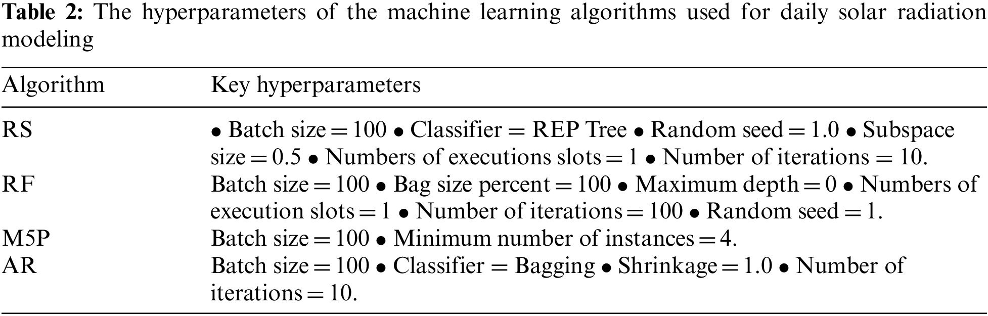
Additive regression (AR) is introduced as a gradient boosting ensemble learning method presented in the WEKA open-source package, which can enhance the predictive performance of a single regressive learner in an iterative process [24]. The AR mechanism includes the iterative enhancement of the regression-based learner by fitting a model in each iteration obtained from the remaining residuals from the previous iteration. Herein, the final prediction is provided by accomplishing the outcomes of every single learner [25]. In this approach, the main hyperparameter is a shrinkage coefficient (learning rate) with a default value equal to 1.0. Reducing the shrinkage coefficient avoids overfitting, and smoothing improves the predictive accuracy. However, selecting a relatively low value of shrinkage coefficient may increase the cost and time computing model [25].

2.1.2 Locally-Weighted Linear Regression

Multilinear regression (MLR), as a supervised learning method, can purpose a linear response between the input variables (xi) and the output one (Zi) in the form of [26]

Zi=ai0+∑m=1Maimxim+εi,m=1:M(1)

where ai0,ai1,…,aim denote the regression coefficients, determined using the least square (LS) method, εi represent the residuals, and M denotes the number of predictors. The fitness function (F) of MLR minimizes the squared error between the observed output (Z om) and the estimated one (Z o), which is expressed as follows

MinimizeF=12M∑m=1M(Z om−Z m)2(2)

In the case of nonlinear relationships between input variables and target ones, MLR becomes less efficient. The locally-weighted linear regression (LWLR) method introduced here is considered a non-parametric lazy learning method. LWLR is an advanced extension of the MLR approach, proposed for the first time by Atkinson et al. [27] to overcome the drawbacks of conventional MLR. A weight function captures the existing non-linearity relationship between the training data set and the target variable in this approach. For this purpose, a fitness function is described as follows [28,29]

Fitness=12M∑m=1MWm(Zom−Zm)2(3)

where W is the weight function. This fitness function can be defined in a matrix form as (Xφ−Z)TW(Xφ−Z), where X and Z denote the input matrix and output vector, respectively. In order to minimize the fitness function, it is required to differentiate the mentioned function over φ and set the XTW(Xφ−Z) matrix function to zero. Thus, φ can be obtained as [29]

φ=(XTWX)−1XTWZ(4)

Here, the radial basis (Gaussian) kernel function (WRBF) is used to replace the weighted matrix. This function is expressed as

WRBF,ij=exp⁡(−γ(xi−xj)2)(5)

in which, γ denotes a constant number, whereas (xi−xj) stands for the difference between pairs of data points (i and j).

2.1.3 M5P Model

The M5P model extends the M5 tree decision model [30], first developed by Wang et al. [31] to solve regression problems. In the M5P model, traditional decision trees are combined using linear regression functions at the leaf points of the trees. The most crucial advantage of decision tree models is their ability to solve nonlinear problems with extensive data and features for regression tasks [32]. Herein, the data space is split into smaller sub-spaces to generate the decision tree for each particular sub-space using the elements comprised of nodes, roots, leaves, and branches. In the M5P process, the linear regression functions provided for various sub-spaces construct a set of linear models (as a committee machine) to capture the existing non-linearity. Generally, the training process of the M5P algorithm comprises three steps generating, pruning, and smoothing decision trees. The M5P model is executed using the maximization of a criterion so-called the standard reduction (SDR), as follows

SDR=SD(τ)−∑i=1N(τiτ)SD(τi)(6)

in which, τ denotes the data samples, τi denotes the ith sub-space associated with a leaf, and SD denotes the standard deviation. It is noteworthy that a pre-scribed value of SDR terminates the training phase. Besides, the useless leaves are pruned during the training phase to avoid overfitting. In the last stage, the unavoidable discontinuities between adjacent leaves are compensated for by a smoothing procedure [30]. The flowchart of the M5P model is demonstrated in Fig. 1.

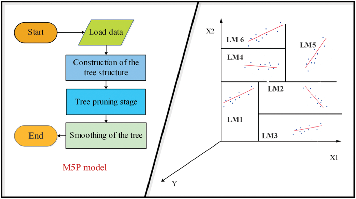
Figure 1: Flowchart of M5P model (left) and a sample of linear regression functions in sub-spaces (right)

2.1.4 Random Forest

Random forest (RF) is a flexible bootstrap aggregated (bagged) ensemble machine learning approach, widely implemented for many regression and classification tasks. RF incorporates a forest of random binary trees based on the Classification and Regression Trees (CART) algorithm and a bagging strategy to enhance standalone CART accuracy, as shown in Fig. 2. Many researchers have recently welcomed the simple mechanism of this method in solving significant nonlinear problems concerning its ability to mitigate bias and error to variance [23]. CART models, in many cases, lead to overfitting and instability during the training. In the RF approach, and for overcoming these drawbacks and reducing the error of each tree model, the bagging strategy is used based on two random operators. In the first operator, a subset of training data Ψ is randomly selected to construct each independent decision tree D(.,Ψi), which can be expressed as [32,33]

{D(X,Ψ1)},{D(X,Ψ2)},….,{D(X,Ψm)};i=1:m(7)

where, X and m are the training data and the number of decision trees, respectively. During the training stage, the values D(X,Ψn) are iteratively updated at the leaf nodes through a weighted average process, i.e.,

Wi(X,Ψ)=Xi∑Xi;i=1,2,…,m;∑Wi=1(8)

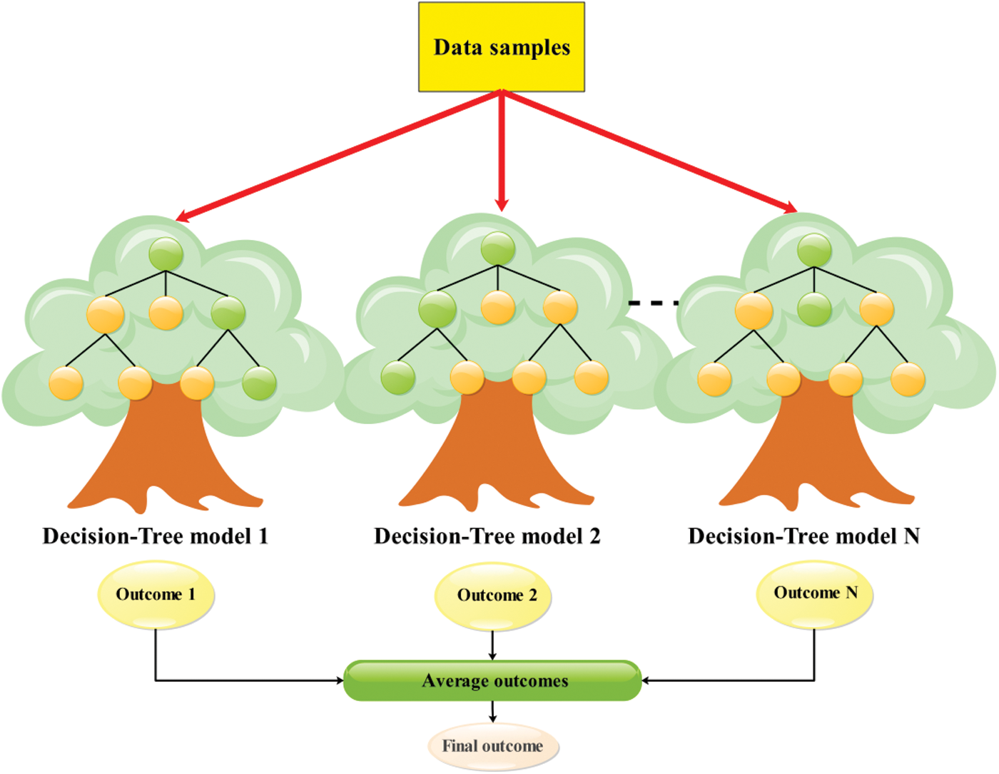
Figure 2: RF flowchart of regression problems

Each input variable introduced to a decision tree in the second operator leads to an independent decision. Consequently, the final response of RF is generated using the majority voting in classification tasks or by averaging individual predictions of decision trees in regression. For regression tasks, this is expressed as [34]

OX=∑i=1m1nWi(X,Ψ)Yi(9)

Finally, the rest of the data which did not participate in the training phase of the decision trees is used to compute the out-of-bag (OOB) error and examine the accuracy of the RF model. Here, two tuning hyperparameters, namely the number of trees in the forest and the number of predictors in each tree, were considered, which should be carefully selected to avoid overfitting. The reader is referred to [26,27] for more detail about the RF approach.

2.1.5 Random Subspace

Random subspace (RS) or “attribute bagging” method is an ensemble machine learning approach similar to the bagging algorithm. The primary strategy of RS is to reduce the correlation between estimators. Some features are randomly selected instead of the whole feature subset during the training stage [35]. In the RS model, an attempt is made to combine the single generated models obtained from the learners, in a single model with superior performance, compared to the performances of individual learners [36]. As mentioned before, as in the bagging method, each learner randomly selects a subset of the training data set, considering replacement, which is the main difference from the bagging method [37]. This method is a suitable option for solving high-dimensional problems. The number of attributes (features) is significant compared to training data points [38]. To construct an ensemble model based on the RS strategy, the following steps are followed [39]:

1: Let N be the training data points, and D be the number of features in the training data sets.

2: Let L be the number of standalone learners for constructing the ensemble model.

3: Chose a subset of input data points (ni) for each (standalone) learner (i), with ni<N.

4: Allocate a training subset for each learner by considering di features (di<D).

5: Combine the predictions of the L standalone learners using majority voting techniques for developing an ensemble model.

2.2 Developed Models

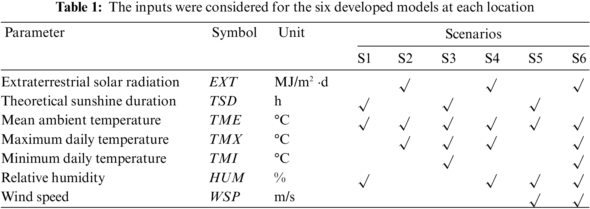
The developed models are based on six different combinations (scenarios) of input variables, as shown in Tab. 1. Besides, the extraterrestrial solar radiation (EXT) and the theoretical sunshine duration (TSD) in Tab. 1 are calculated mathematically using the date and time stamps of the data, as demonstrated in [23]. For each set of inputs, four hybrid models have been developed by integrating additive regression with RF, RS, LWLR, and M5P. Tab. 2 shows the optimized hyperparameters of these models. The datasets for each location were divided into two subsets for training and testing. The training stage corresponds to the recorded data from 2007 to 2012, while the testing stage employed the data from 2013 to 2015.

The accuracy and suitability of the models were assessed using the root mean square error (RMSE), the relative RMSE (RRMSE), and Pearson correlation coefficient (R) of the linear regression forced to the origin of the n pairs of observed and predicted GSR values, mean absolute error (MAE) [40–45].

2.3 Collected Data and Studied Area

This study is carried out for the region of Andalusia, located in the south of the Iberian Peninsula. Andalusia covers a land area of about 87268 km2 with a complex climate [46]. The total annual rainfall ranges from <300 mm (southeast coast) to >1000 mm (Betic mountains, Sierra Morena). The region has mild temperatures, with average annual temperatures above 17°C and 13°C in Sierra Morena and Betic mountains, respectively, and 300 days of sunshine over most of the territory. The stations with semi-arid climates were selected for this work, as shown in Tab. 3. A semi-arid climate, also known as a semi-desert or steppe climate, occurs when precipitation is less than possible evapotranspiration but not as low as in an arid desert climate. Semi-arid climates come in various forms, giving rise to various biomes depending on air temperature. The Köppen Climate Classification’s subtype for this climate is BS [47].

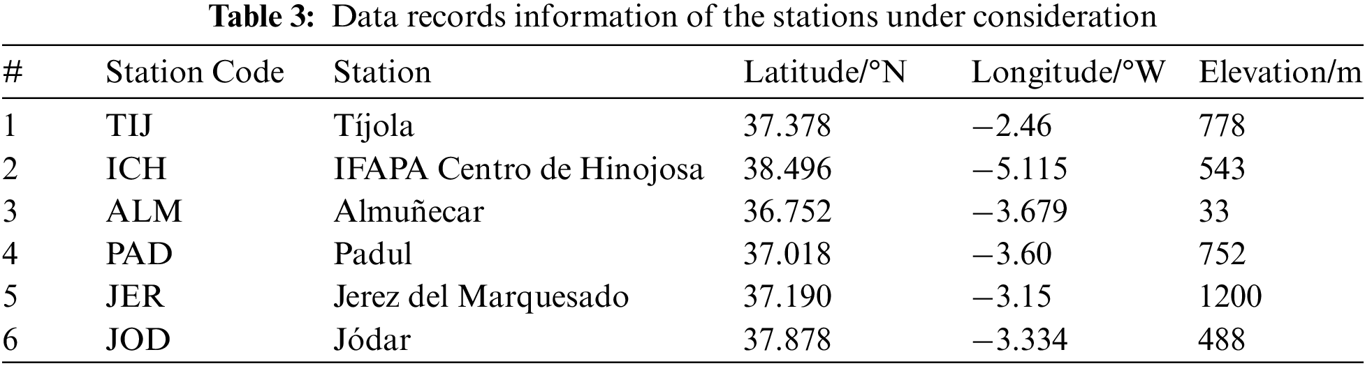
The measured meteo-solar radiation datasets for the six locations in Tab. 3 were obtained from the Spain Agroclimatic Information Network (SIAR; Sistema de Información Agroclimática para el Regadío, available at: https://eportal.mapa.gob.es) for nine years (2007–2015). The quality of the meteorological values of each station is tested through different checks, including range, step, internal consistency, persistence, and spatial consistency [48]. The correlograms in Fig. 3 demonstrate the strength of linear correlations between these variables and the predicted one (GSR).

This Figure, EXT stands for the daily extraterrestrial solar radiation, whereas TSD stands for the theoretical sunshine duration.

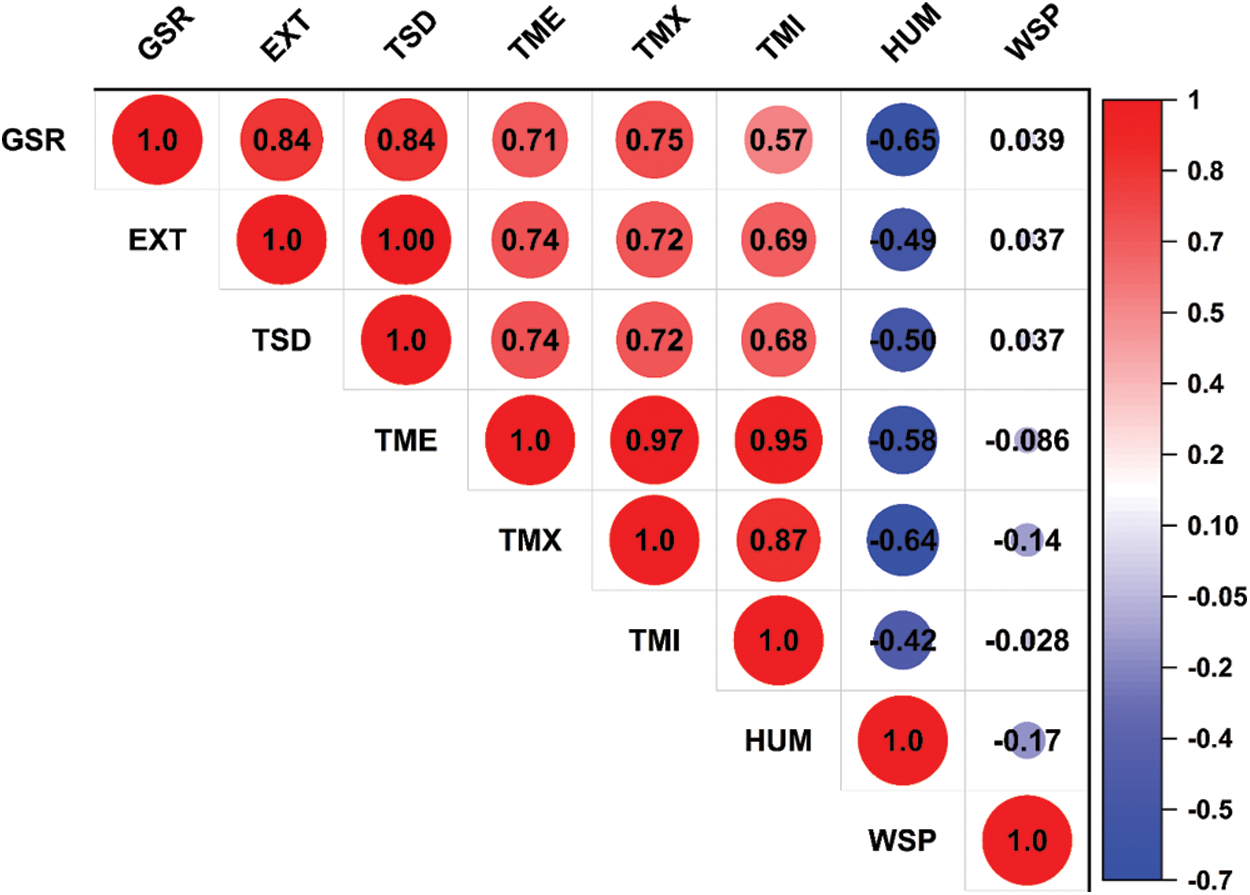
Figure 3: Correlograms of meteorological variables considering the combined dataset of all stations

3  Results and Discussion

This section provides the detailed results of the afore-described models in both the training and testing stages. The six models (S1 to S6) are first developed for the first four locations (TIJ, ICH, ALM, and PAD). The most promising models and base algorithms are highlighted. Those selected models are further verified at the other locations (JER and JOD).

3.1 Evaluation of Different Hybrid Models

As shown in Fig. 4a, four hybrid models have been developed by integrating the additive regression algorithm with the four-machine learning, overviewed in Section 2.1. The Figure shows the sixth scenario/model results in the training phase, with all seven variables considered as the inputs. The Figure shows appreciable differences in the performances of all models, which justifies the objective of this study, i.e., exploring new base algorithms for considerable improvement in prediction accuracy. Fig. 4a also highlights considerable differences between models’ performances at different locations, with TIJ and ICH showing better error estimates than ALM and PAD. This also contributes to the significance of this study, where such discrepancies in models’ performances occur within the same climatic zone, let alone across different zones. Compared to all other models, the AR-RF model shows exceptional performance in terms of RRMSE error measure with RRMSE values as low as 10.950% (at ICH) and also exceeds the performances of other models by up to 50.5% in terms of RRMSE. These substantial improvements emphasize the importance of the model hybridization concept and selecting the base algorithms of the hybrid model [49,50]. For instance, Fig. 4a shows that the AR-M5P models always result in the least accurate predictions, even though M5P and RF (best-performing base algorithm) share the base foundation of decision trees. It is also depicted that the AR-RS model performs close to the AR-RF model. In contrast, and at this point, AR-LWLR and AR-M5P models show significantly poor performances compared to the other models. Hence, they are excluded from the following discussions.

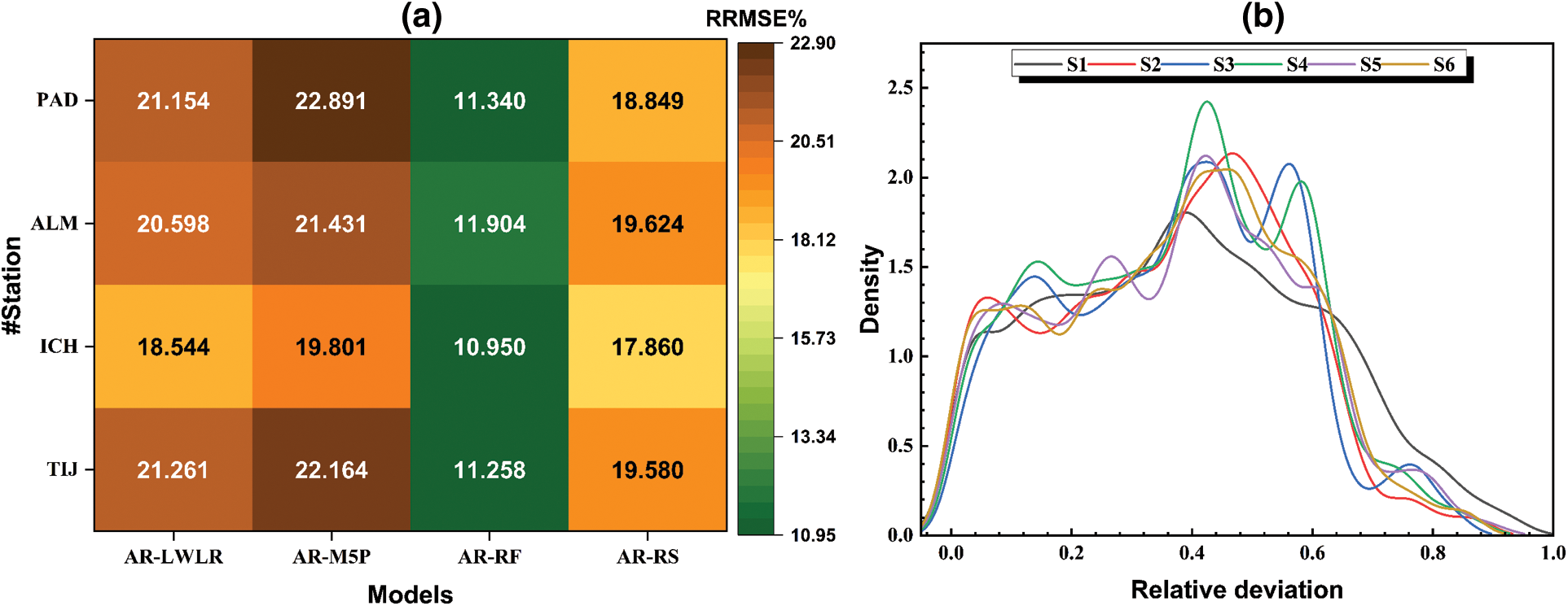
Figure 4: Prediction errors of all models/scenarios: (a) RRMSE values of all hybrid models, and (b) distributions of the relative prediction errors of all models (with different subsets of inputs)

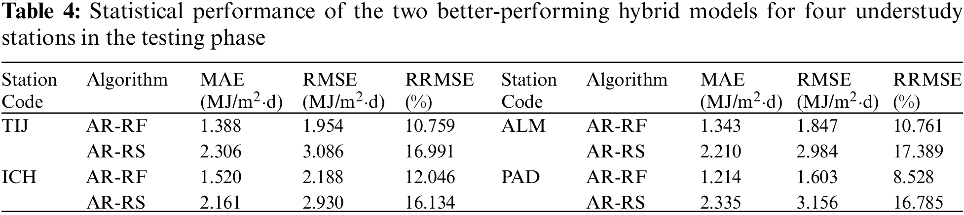
So far, the models have been discussed, considering their performance in the training phase. However, their performance in the testing phase is more important to see if they can handle new observations with different statistics. Tab. 4 summarizes the error estimates of the two best-performing models (i.e., AR-RF and AR-RS) when tested using the three years (2013 to 2015) datasets at the four locations. Once again, the AR-RF models show superior performances compared to the AR-RS models, with improvements up to 52.9% and 54.2% in terms of MAE and RMSE, respectively. Most importantly, the AR-RF model shows a highly stable performance when processing the datasets for three years of the testing phase. Typically, data-driven models tend to have higher error estimates in the test phase since they are not necessarily prepared for new data points that they have not been trained to handle. However, since the model is well-developed and the two datasets of training and validation are large enough, the model shows comparable error estimates at ICH (e.g., training and testing RMSEs of 1.902 and 2.188 MJ/m2.day). Even lower test error estimates at the three other locations. For instance, at PAD, the RMSE of the testing phase (1.603 MJ/m2⋅day) is 20.1% lower than that of the training phase (2.024 MJ/m2⋅day). The AR-RF model demonstrates excellent performance at this location (PAD), with an RRMSE of only 8.5%. Overall, it is concluded that the AR-RF models are the most suitable for such climatic conditions, followed by AR-RS, which is also a bagging technique.

3.2 Impact of Model Inputs

So far, the different hybrid models have been assessed based on the input variables of Scenario #6, where wind speed and relative humidity records are also required. Also, from the previous section, it has been demonstrated that AR-RF results in sustainably better predictions of GSR. Hence, this section aims to evaluate the sensitivity of the AR-RF model’s predictions to different input combinations. As shown in Fig. 4b, the six combinations of model inputs result in different but comparable density distributions of residuals. As aforementioned, all models tend to overestimate the actual GSR values. However, the more complex models (S4 to S6) tend to show less frequent significant overestimations, as clear from the shifted peaks to the left in Fig. 4b.

To better summarize the performance of the models with different inputs, Fig. 5 shows the Taylor diagrams of the six models at TIJ, ICH, ALM, and PAD. The model’s performance improves as the number of inputs increases, especially when the new inputs represent a brand-new domain/type of measurements. This is expected since data-driven models tend to be greedy regarding dataset size and the number of inputs. S1 and S2 show lower performances for most stations, whereas S6 performs considerably better. However, the differences between models S3 to S6 are not that significant. Hence, all are recommended depending on the anticipated level of accuracy in GSR predictions, with S6 being the most accurate (but requires additional measurements of wind speed and relative humidity) and S3 being the most cost-effective (only air temperature measurements are required). The comparable performances of S3 and S6 are even clearer in Fig. 6. In this Figure, while all models fail to capture extreme GSR values, they succeed in capturing the actual GSR records’ main distribution characteristics (e.g., mean and quartile values).

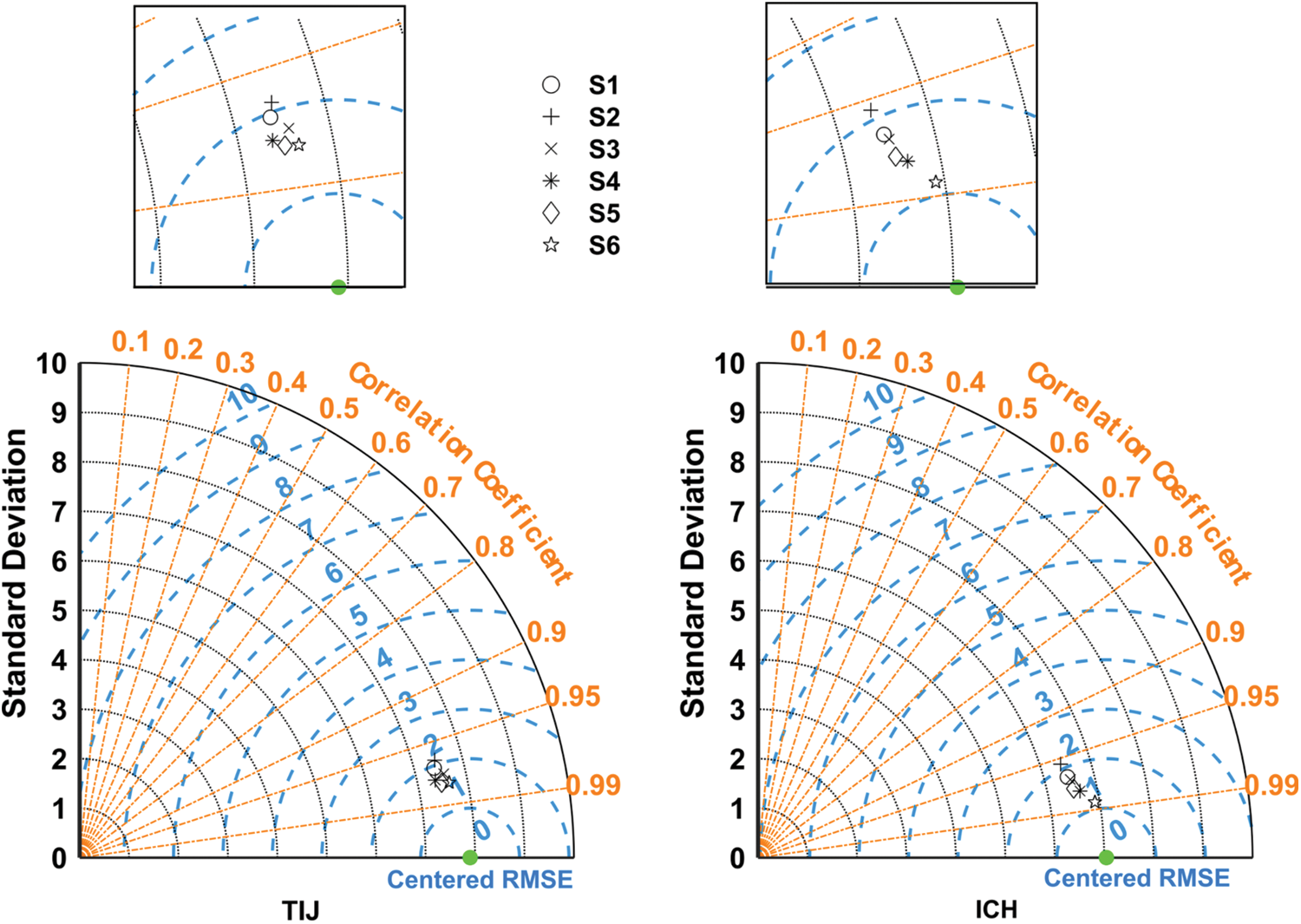
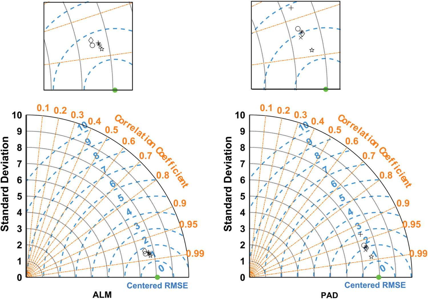
Figure 5: Taylor diagrams of all scenarios for the four training locations in the test phase

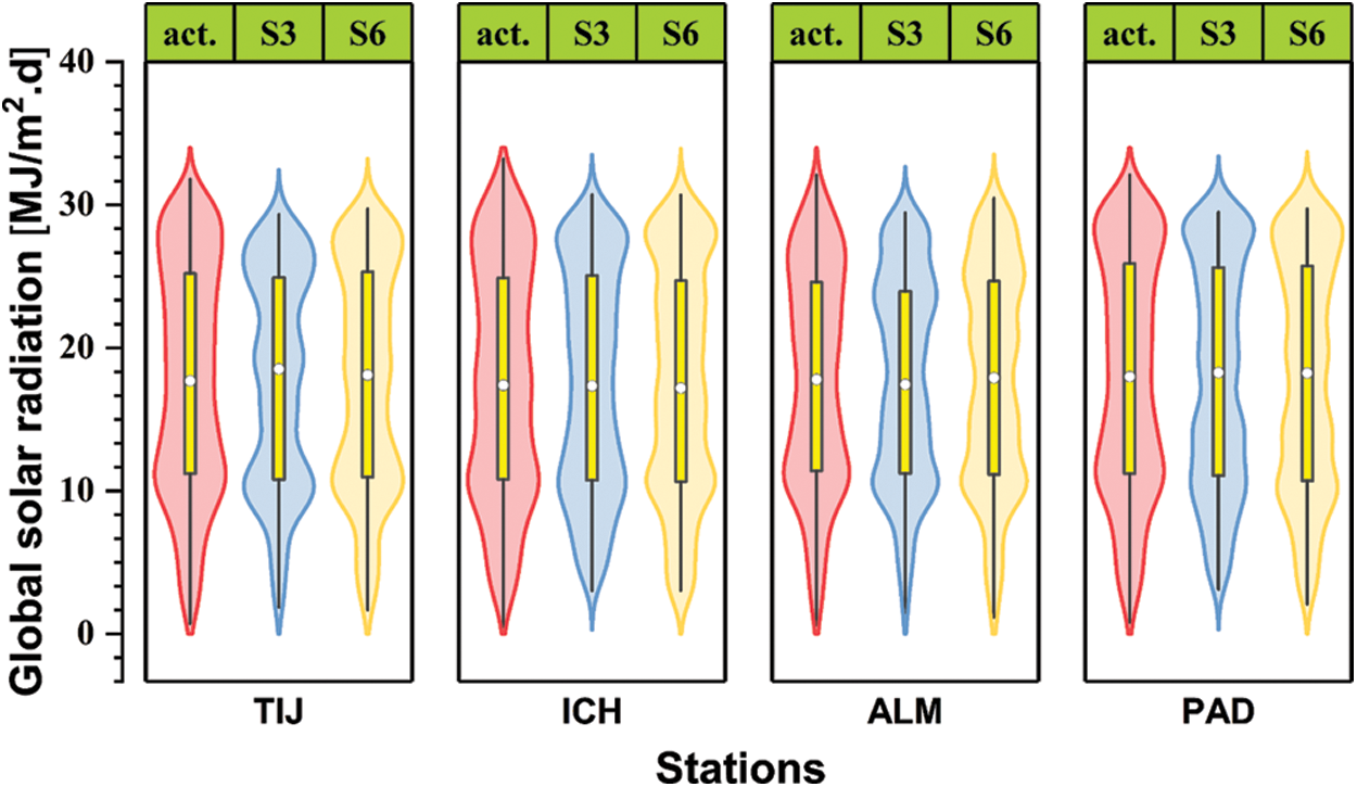
Figure 6: Violin plots of models S3 and S6 for the four selected locations in the test phase

3.3 Verification at New Locations

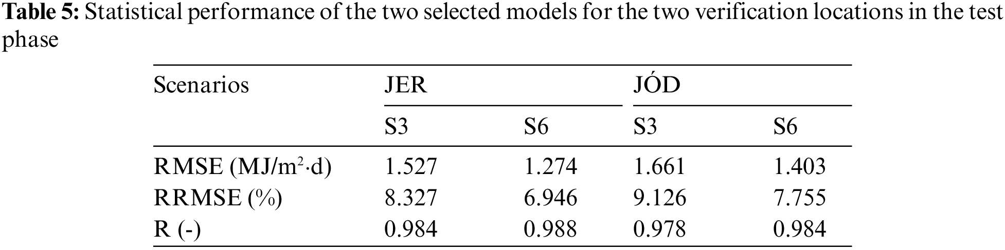
As a final verification of the selected models (AR-RF models based on S3 and S6 input combinations), the error estimates of the test phase are summarized in Tab. 5. Compared to the results in Tab. 4, it can be seen that even better error estimates are obtained at the two new locations (JER and JOD), with RMSEs as low as 1.274 MJ/m2⋅day (the lowest RMSE in Tab. 4 was 1.603 MJ/m2⋅day for PAD). The RRMSE values are also substantially lower than those in Tab. 4. This proves that the suggested models are generalizable to distant locations with similar climatic features. Once again, S6 shows the best performances, with RMSEs of 1.274 and 1.403 MJ/m2⋅day at JER and JOD, respectively. However, these values are in the same order of magnitude as those offered by S3, which is drastically simpler. Hence, the AR-RF model based on air temperature measurements (S3) is recommended as the best trade-off between complexity and accuracy.

4  Conclusions

In this research, four novel hybrid ensemble models based on RS, RF, M5P, and LWLR, each integrated with AR (i.e., AR-RS, AR-RF, AR-M5P, and AR-LWLR), were developed to estimate the solar radiation for six semi-arid regions of Spain. Extraterrestrial solar radiation, theoretical sunshine duration, mean ambient temperature, maximum daily temperature, minimum daily temperature, relative humidity, and wind speed were employed as the input variables. First, four hybrid ensemble models were examined based on all input parameters in four stations (TIJ, ICH, ALM, and PAD) during the training phase. The results show that the AR-M5P models have the lowest accuracy, with correlation coefficients of only 0.874, 0.909, 0.870, and 0.869 at TIJ, ICH, ALM, and PAD. In contrast, the testing phase outcomes demonstrated that the AR-RF models have the best performances among all the hybrid models, with correlation coefficients of 0.97, 0.962, 0.966, and 0.982 at the same locations, respectively. In the next stage, six scenarios (input combinations: S1:S6) based on a correlation analysis were adopted to examine AR-RF, as the superior ensemble model, at two remaining stations (i.e., JER and JOD) to verify the model’s performance and assess the impact of candidate inputs on the prediction accuracy. The testing phase results proved that Scenario #6 leads to the highest accuracy, compared to other scenarios, with RMSEs of 1.274 and 1.403 MJ/m2⋅day and correlation coefficients of 0.988 and 0.968 at JER and JOD, respectively. Also, Scenario #3 stood in the next rank of accuracy for estimating the solar radiation in both validating stations. The AD-RF was the best predictive model, followed by AD-RS. However, the AD-RF model has better performance than all other models for most stations. Therefore, predicting global solar radiation for regions with similar climate characteristics using AD-RS is recommended.

Acknowledgement: The authors acknowledge the Agroclimatic-Information-Network of Andalusia (RIA) in providing most of the used data. This work was supported by the Portuguese Foundation for Science and Technology (FCT) through the project PTDC/CTA-OHR/30561/2017 (WinTherface).

Funding Statement: The authors received no specific funding for this study.

Conflicts of Interest: The authors declare that they have no conflicts of interest to report regarding the present study.

References

1. W. Qin, L. Wang, A. Lin, M. Zhang, X. Xia et al., “Comparison of deterministic and data-driven models for solar radiation estimation in China,” Renewable and Sustainable Energy Reviews, vol. 81, no. 17, pp. 579–594, 2018. [Google Scholar]
2. C. A. Gueymard and D. R. Myers, “Evaluation of conventional and high-performance routine solar radiation measurements for improved solar resource, climatological trends, and radiative modeling,” Solar Energy, vol. 83, no. 2, pp. 171–185, 2009. [Google Scholar]
3. K. Bouchouicha, M. A. Hassan, N. Bailek and N. Aoun, “Estimating the global solar irradiation and optimizing the error estimates under Algerian desert climate,” Renewable Energy, vol. 139, no. 1, pp. 844–858, 2019. [Google Scholar]
4. S. Lou, Y. Huang, D. H. W. Li, D. Xia, X. Zhou et al., “A novel method for fast sky conditions identification from global solar radiation measurements,” Renewable Energy, vol. 161, no. 1, pp. 77–90, 2020. [Google Scholar]
5. N. Bailek, K. Bouchouicha, Y. A. Abdel-Hadi, M. El-Shimy, A. Slimani et al., “Developing a new model for predicting global solar radiation on a horizontal surface located in Southwest region of Algeria,” NRIAG Journal of Astronomy and Geophysics, vol. 9, no. 1, pp. 341–349, 2020. [Google Scholar]
6. S. Samadianfard, A. Majnooni-Heris, S. N. Qasem, O. Kisi, S. Shamshirband et al., “Daily global solar radiation modeling using data-driven techniques and empirical equations in a semi-arid climate,” Engineering Applications of Computational Fluid Mechanics, vol. 13, no. 1, pp. 142–157, 2019. [Google Scholar]
7. J. Almorox, J. A. Arnaldo, N. Bailek and P. Martí, “Adjustment of the Angstrom-Prescott equation from Campbell-Stokes and Kipp-Zonen sunshine measures at different timescales in Spain,” Renewable Energy, vol. 154, no. 1, pp. 337–350, 2020. [Google Scholar]
8. B. Keshtegar, K. Bouchouicha, N. Bailek, M. A. Hassan, R. Kolahchi et al., “Solar irradiance short-term prediction under meteorological uncertainties: Survey hybrid artificial intelligent basis music-inspired optimization models,” The European Physical Journal Plus, vol. 137, no. 3, pp. 22–40. 2022. [Google Scholar]
9. F. Besharat, A. A. Dehghan and A. R. Faghih, “Empirical models for estimating global solar radiation: A review and case study,” Renewable and Sustainable Energy Reviews, vol. 21, no. 1, pp. 798–821, 2013. [Google Scholar]
10. K. Bouchouicha, N. Bailek, M. E. Mahmoud, J. A. Alonso, A. Slimani et al., “Estimation of monthly average daily global solar radiation using meteorological-based models in Adrar, Algeria,” Applied Solar Energy, vol. 54, no. 6, pp. 448–455, 2018. [Google Scholar]
11. H. Sun and R. Grishman, “Employing lexicalized dependency paths for active learning of relation extraction,” Intelligent Automation & Soft Computing, vol. 34, no. 3, pp. 1415–1423, 2022. [Google Scholar]
12. B. Dalal, A. Bagui and S. Sengupta, “Meteorological data driven prediction of global solar radiation,” in Second Int. Conf. on Control, Measurement and Instrumentation (CMI), Kolkata, India, pp. 184–189, 2021. [Google Scholar]
13. M. Santamouris, G. Mihalakakou, B. Psiloglou, G. Eftaxias and D. N. Asimakopoulos, “Modeling the global solar radiation on the earth’s surface using atmospheric deterministic and intelligent data-driven techniques,” Journal of Climate, vol. 12, no. 10, pp. 3105–3116, 1999. [Google Scholar]
14. M. A. Hassan, N. Bailek, K. Bouchouicha and S. C. Nwokolo, “Ultra-short-term exogenous forecasting of photovoltaic power production using genetically optimized non-linear auto-regressive recurrent neural networks,” Renewable Energy, vol. 171, no. 1, pp. 191–209, 2021. [Google Scholar]
15. E. M. El-Kenawy, A. Ibrahim, N. Bailek, K. Bouchouicha, M. A. Hassan et al., “Hybrid ensemble-learning approach for renewable energy resources evaluation in Algeria,” Computers, Materials & Continua, vol. 71, no. 3, pp. 5837–5854, 2022. [Google Scholar]
16. E. M. El-kenawy, A. Ibrahim, N. Bailek, K. Bouchouicha, M. A. Hassan et al., “Sunshine duration measurements and predictions in Saharan Algeria region: An improved ensemble learning approach,” Theoretical and Applied Climatology, vol. 147, no. 3, pp. 1015–1031, 2022. [Google Scholar]
17. M. Vakili, S. R. Sabbagh-Yazdi, S. Khosrojerdi and K. Kalhor, “Evaluating the effect of particulate matter pollution on estimation of daily global solar radiation using artificial neural network modeling based on meteorological data,” Journal of Cleaner Production, vol. 141, no. 1, pp. 1275–1285, 2017. [Google Scholar]
18. J. Yeom, S. Park, T. Chae, J. Kim and C. S. Lee, “Spatial assessment of solar radiation by machine learning and deep neural network models using data provided by the COMS MI geostationary satellite: A case study in South Korea,” Sensors, vol. 19, no. 9, pp. 2082, 2019. [Google Scholar]
19. I. N. Kosovic, T. Mastelic and D. Ivankovic, “Using artificial intelligence on environmental data from internet of things for estimating solar radiation: Comprehensive analysis,” Journal of Cleaner Production, vol. 266, no. 1, pp. 121489, 2020. [Google Scholar]
20. N. Al-Rousan, H. Al-Najjar and O. Alomari, “Assessment of predicting hourly global solar radiation in Jordan based on rules, trees, meta, lazy and function prediction methods,” Sustainable Energy Technologies and Assessments, vol. 44, no. 20, pp. 100923, 2021. [Google Scholar]
21. M. Taki, A. Rohani and H. Yildizhan, “Application of machine learning for solar radiation modeling,” Theoretical and Applied Climatology, vol. 143, no. 3, pp. 1599–1613, 2021. [Google Scholar]
22. M. A. Hassan, A. Khalil, S. Kaseb and M. A. Kassem, “Potential of four different machine-learning algorithms in modeling daily global solar radiation,” Renewable Energy, vol. 111, no. 1, pp. 52–62, 2017. [Google Scholar]
23. M. A. Hassan, A. Khalil, S. Kaseb and M. A. Kassem, “Exploring the potential of tree-based ensemble methods in solar radiation modeling,” Applied Energy, vol. 203, no. 1, pp. 897–916, 2017. [Google Scholar]
24. J. H. Friedman, “Stochastic gradient boosting,” Computational Statistics & Data Analysis, vol. 38, no. 4, pp. 367–378, 2002. [Google Scholar]
25. A. Varnek, Tutorials in Chemoinformatics, Hoboken, New Jersey, USA: John Wiley & Sons, 2017. [Google Scholar]
26. I. Ahmadianfar, M. Jamei and X. Chu, “A novel hybrid wavelet-locally weighted linear regression (W-LWLR) model for electrical conductivity (EC) prediction in water surface,” Journal of Contaminant Hydrology, vol. 232, no. 1, pp. 103641, 2020. [Google Scholar]
27. C. G. Atkeson, A. W. Moore and S. Schaal, “Locally weighted learning for control,” Artificial Intelligence Review, vol. 11, no. 5, pp. 75–113, 1997. [Google Scholar]
28. I. Ahmadianfar, M. Jamei and X. Chu, “Prediction of local scour around circular piles under waves using a novel artificial intelligence approach,” Marine Georesources & Geotechnology, vol. 40, no. 2, pp. 1–12, 2019. [Google Scholar]
29. M. Jamei and I. Ahmadianfar, “Prediction of scour depth at piers with debris accumulation effects using linear genetic programming,” Marine Georesources & Geotechnology, vol. 38, no. 4, pp. 468–479, 2020. [Google Scholar]
30. J. Quinlan, “Learning with continuous classes,” in Proc. of the 5th Australian Joint Conf. on Artificial Intelligence, Hobart, Tasmania, Australia, pp. 343–348, 1992. [Google Scholar]
31. Y. Wang and I. H. Witten, Induction of Model Trees for Predicting Continuous Classes, Hamilton, New Zealand: University of Waikato, Department of Computer Science, pp. 23, 1996. [Google Scholar]
32. I. Ahmadianfar, M. Jamei, M. Karbasi, A. Sharafati and B. Gharabaghi, “A novel boosting ensemble committee-based model for local scour depth around non-uniformly spaced pile groups,” Engineering with Computers, vol. 10, no. 1, pp. 1–23, 2021. [Google Scholar]
33. L. Breiman, “Random forests,” Machine Learning, vol. 45, no. 1, pp. 5–32, 2001. [Google Scholar]
34. L. Guo, N. Chehata, C. Mallet and S. Boukir, “Relevance of airborne lidar and multispectral image data for urban scene classification using random forests,” ISPRS Journal of Photogrammetry and Remote Sensing, vol. 66, no. 1, pp. 56–66, 2011. [Google Scholar]
35. J. Mielniczuk and P. Teisseyre, “Using random subspace method for prediction and variable importance assessment in linear regression,” Computational Statistics & Data Analysis, vol. 71, no. 1, pp. 725–742, 2014. [Google Scholar]
36. X. Zhang and Y. Jia, “A linear discriminant analysis framework based on random subspace for face recognition,” Pattern Recognition, vol. 40, no. 9, pp. 2585–2591, 2007. [Google Scholar]
37. A. Bertoni, R. Folgieri and G. Valentini, “Bio-molecular cancer prediction with random subspace ensembles of support vector machines,” Neurocomputing, vol. 63, no. 1, pp. 535–539, 2005. [Google Scholar]
38. Y. Piao, M. Piao, C. H. Jin, H. Sun Shon, J. Chung et al., “A new ensemble method with feature space partitioning for high-dimensional data classification,” Mathematical Problems in Engineering, vol. 25, no. 1, pp. 50–59, 2015. [Google Scholar]
39. L. I. Kuncheva, J. J. Rodríguez, C. O. Plumpton, D. E. J. Linden and S. J. Johnston, “Random subspace ensembles for fMRI classification,” IEEE Transactions on Medical Imaging, vol. 29, no. 2, pp. 531–542, 2010. [Google Scholar]
40. A. Naseri, M. Jamei, I. Ahmadianfar and M. Behbahani, “Nanofluids thermal conductivity prediction applying a novel hybrid data-driven model validated using Monte Carlo-based sensitivity analysis,” Engineering with Computers, vol. 38, no. 1, pp. 815–839, 2022. [Google Scholar]
41. W. Sun, L. Dai, X. Zhang, P. Chang and X. He, “RSOD: Real-time small object detection algorithm in UAV-based traffic monitoring,” Applied Intelligence, vol. 52, no. 1, pp. 8448–8463, 2022. [Google Scholar]
42. A. Elbeltagi, B. Zerouali, N. Bailek, K. Bouchouicha, C. Pande et al., “Optimizing hyperparameters of deep hybrid learning for rainfall prediction: A case study of a Mediterranean basin,” Arabian Journal of Geosciences, vol. 15, no. 10, pp. 933, 2022. [Google Scholar]
43. M. Guermoui, K. Bouchouicha, N. Bailek and J. W. Boland, “Forecasting intra-hour variance of photovoltaic power using a new integrated model,” Energy Conversion and Management, vol. 245, no. 1, pp. 114569, 2021. [Google Scholar]
44. N. Aoun, K. Bouchouicha and N. Bailek, “Seasonal performance comparison of four electrical models of monocrystalline PV module operating in a harsh environment,” IEEE Journal of Photovoltaics, vol. 9, no. 4, pp. 1057–1063, 2019. [Google Scholar]
45. N. Bailek, K. Bouchouicha, M. A. Hassan, A. Slimani and B. Jamil, “Implicit regression-based correlations to predict the back temperature of PV modules in the arid region of south Algeria,” Renewable Energy, vol. 156, no. 1, pp. 57–67, 2020. [Google Scholar]
46. J. Gómez-Zotano, J. Alcántara-Manzanares, E. Martínez-Ibarra and J. A. Olmedo-Cobo, “Applying the technique of image classification to climate science: The case of Andalusia (Spain),” Geographical Research, vol. 54, no. 4, pp. 461–470, 2016. [Google Scholar]
47. M. C. Peel, B. L. Finlayson and T. A. McMahon, “Updated world map of the Köppen-Geiger climate classification,” Hydrology and Earth System Sciences, vol. 11, no. 5, pp. 1633–1644, 2007. [Google Scholar]
48. J. Estévez, P. Gavilán and J. V. Giráldez, “Guidelines on validation procedures for meteorological data from automatic weather stations,” Journal of Hydrology, vol. 402, no. 2, pp. 144–154, 2011. [Google Scholar]
49. E. M. El-kenawy, B. Zerouali, N. Bailek, K. Bouchouicha, M. A. Hassan et al., “Improved weighted ensemble learning for predicting the daily reference evapotranspiration under the semi-arid climate conditions,” Environmental Science and Pollution Research, vol. 29, pp. 1–21, 2022. [Google Scholar]
50. H. Sun and R. Grishman, “Lexicalized dependency paths based supervised learning for relation extraction,” Computer Systems Science and Engineering, vol. 43, no. 3, pp. 861–870, 2022. [Google Scholar]
Cite This Article
Copyright © 2023 The Author(s). Published by Tech Science Press.
This work is licensed under a Creative Commons Attribution 4.0 International License , which permits unrestricted use, distribution, and reproduction in any medium, provided the original work is properly cited.
Downloads
Citation Tools