Deep Learned Singular Residual Network for Super Resolution Reconstruction

1  Introduction

Image resolution is usually described in terms of pixels per inch (PPI). For a given image, PPI displays the number of pixels available. A greater PPI signifies a higher resolution and provides higher pixel information that produces sharp images of high-quality. Low resolution (LR) images have fewer pixels and less detail. Sensor native resolution, under-sampling with low-cost sensors, sub-optimal accession such as camera shake, and unpleasant light are the key factors that limit the quality of an image. These factors lead to LR images in which fine and detailed information is lost. So, it is desired to produce images of higher resolution than the imaging device. Over the years, super resolution (SR) algorithms have gained a lot of attention due to their widespread applications [1–3] in remote sensing, object detection [4], surveillance monitoring, etc. Single image super resolution (SISR) techniques aim to recover images of higher resolution from the corresponding LR images.

Over the past decades, various approaches to SISR have been proposed. Primarily, interpolation methods [5] such as nearest neighbor, bicubic, and bilinear have a specific advantage of requiring less computing effort because of their simplicity. These interpolation-based methods work well in smooth or low frequency areas but worse in high frequency areas such as edge regions. Because they are prone to blur and aliasing artifacts along the edges. For the upscaling of LR image size, these methods use nonparametric or parametric methods, and the generation of high resolution (HR) image involves the application of a default interpolation kernel to evaluate the pixels of the HR grid. Interpolation methods including bicubic or bilinear have a tendency to produce very smooth images with ringing and jagged artifacts which hinders their applications. Interpolation using natural prior images usually produces favorable results and works well to preserve the edges of the enlarged image. Even so, real-world images involve limitations in simulating their visual complexity and tend to result in watercolor-like traces. As a result, the capability of these SR methods is limited. Rational fractal interpolation (RFI) [6,7] preserves texture details, and the performance of the RFI kernel is more efficient than polynomial kernels. Even so, the interpolation methods show inferior performance compared to the learning-based methods.

Reconstruction based methods [8–10] can achieve good results with edge preservation if reasonable preconditions are imposed. These techniques are constantly blended with single or more properly designed priors [11] to anticipate the details overlooked with inside the reconstruction process. These approaches impose reconstruction limitations, requiring that the down sampled and smoothed HR image be near to the LR image. For these methods, image super resolution under local transformations shows explicit limitations in both real and synthetic conditions, and to obtain SR at huge magnification factors, these methods are not favorable. In such cases, the results can be too smooth, missing necessary high frequency data and these methods are usually time-consuming.

Example-based learning [12] is one category of SR methods that applies to an LR image, where the lost high frequency details can be recovered from lower and higher resolution image sample pairs. These methods are built to predetermine a mapping relation between LR feature patches and the corresponding HR responses. The learned mapping relation can predict lost high frequency features in the LR image. To establish the underlying mapping, many methodologies have evolved from existing learning-based methods including sparse coding [13,14] neighbor embedding, nearest-neighbor field [15], linear regression [16], and dictionary learning. In terms of detailed recovery, learning-based techniques are competitive. Unfortunately, the performance is greatly dependent on the training set availability and the training and test set similarity. As these methods involve the dependency on an external database, inappropriate choice of training samples may result in unwanted noises and obvious artifacts.

In recent years, deep learning-based methods [17–37] have been proposed and considered as most promising in the field of SR. Deep learning is a subfield of machine learning that is inspired by the human brain structure. It makes use of multi-layered structures called convolution neural networks. These methods learn how to map noisy images and ground truth mages from end to end to generate high-quality results. Super resolution convolution neural network (SRCNN) involves a lightweight structure of three layers that perform extraction and representation of patches, as well as nonlinear mapping and reconstruction. Very deep super resolution (VDSR) is one of the classical SR approaches that involve the usage of high learning rates such as 104 times more than SRCNN and learns only residuals. It overcomes the limitations of SRCNN such as the context of small regions of image, slow convergence in training, and single scale factor. Enhanced super resolution generative adversarial networks (ESRGAN) architecture contains residual in residual dense blocks without the batch normalization layers and includes residual scaling technique. These make ESRGAN restore more realistic textures and accurate brightness. Because of the ability to extract efficient high-level abstractions bridging LR and HR spaces, modern deep learning-based methods achieved remarkable quantitative and qualitative improvements. Motivated by the strengths of deep learning methods, a framework based on deep learning is proposed to achieve super resolution.

The proposed framework involves the decomposition of input LR image into subbands of singular vectors through singular value decomposition (SVD). These subbands consist of left singular vectors, right singular vectors of low frequency components, and singular values which represent the intensity details of an image. The resultant LR subbands are then fed as input to the trained deep singular-residual neural network (DSRNN) which generates corresponding residual subbands. The HR subbands are produced by combining residuals and LR subbands. Finally, SR image output is generated from these subbands by the application of inverse SVD.

We structure the paper as follows. Section 2 is devoted to dealing with the SVD, architecture, and operation of DSRNN and the SR reconstruction flow. Section 3 involves the discussion of results including datasets used for training and testing, as well as methods and metrics used in the comparison. Finally, our paper concludes in Section 4.

2  Methods

2.1 Singular Value Decomposition

Images can be observed as matrices in which pixels represent the numerical entries. Matrix rows and columns represent the pixel position, while each value in the matrix represents the appropriate saturation level. As a result of these components, a considerable amount of memory may be required to create a single image. So, there is a need for a method so that computers can save images without consuming so much memory. SVD is a popular method used to compress the saturation matrix size while retaining key components to conserve memory while maintaining image quality. It also delivers key theoretical and geometrical insights on linear transformations.

SVD is a linear algebraic operation and involves factorization of a given real or complex matrix I and upon application of SVD, it yields three corresponding sub-matrices as follows.

I=USVT(1)

Image I with size p×q is decomposed into three components U,S, and V, in which U and V are unitary matrices of left and right singular vectors respectively and S is a diagonal matrix containing singular values as shown in Fig. 1. Calculating the SVD involves finding eigenvectors and eigenvalues of I. The eigenvectors of IIT construct the columns of U, the eigenvectors of ITI can construct the columns of V and square roots of eigenvalues of ITI or IIT gives the singular values which are entries of the diagonal of matrix S.

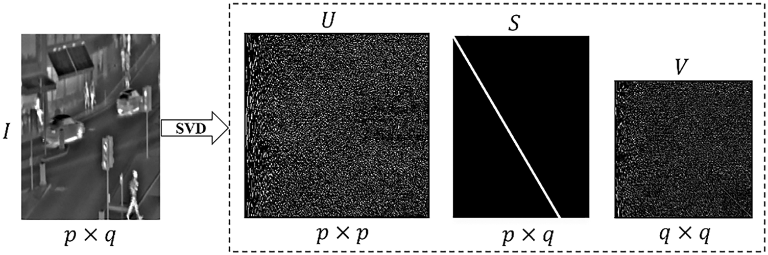
Figure 1: Block diagram of SVD

V is an orthogonal matrix of size q×q such that VT=V−1 which implies VVT=iq. where i represents the identity matrix, VT denotes the transpose which is obtained by swapping the matrix’s rows and columns and V−1 denotes the inverse of matrix V. U is a p×p column orthogonal matrix consisting of orthonormal columns and UTU=ip. S is a diagonal matrix of p×q and consists of non-negative unique singular values as elements along diagonal such as s1,s2,s3,… and stored in a sorted order such that s1≥s2≥s3… These values represent image intensity information. The bigger the value, the more information about the image. The usage of singular values enables us to describe an image with a fewer set of values, storing the essential features and consuming less memory space. Instead of direct usage of LR images, these components produced by SVD are used in the training and testing phases for further analysis.

2.2 Deep Singular-residual Network

In recent years, deep neural networks have shown massive progress in the image processing field. To make the neural network more robust, extract key features from images, and bring down the error rate, more layers are being added. Therefore, it results in a network that is deeper and complex. Due to this, as the depth of architecture increases the performance drops and the network becomes hard to train and resulting in saturation and degradation of accuracy. It is due to the exploding gradient problem which results in becoming, gradient too large or zero. As a result, with the increase in layers, the test and training error rate increases too.

The residual network has shown a tremendous advancement over existing networks in deep learning and resolves the exploding gradient problem. It consists of residual blocks or units which contain skip connections. The basic residual block is represented as shown in Fig. 2a. As the name desires, skip connections skip a few layers, and the output of a layer can be provided to the next layers as the input. By regularization, skip connections help in skipping the layers that affect the performance of the architecture.

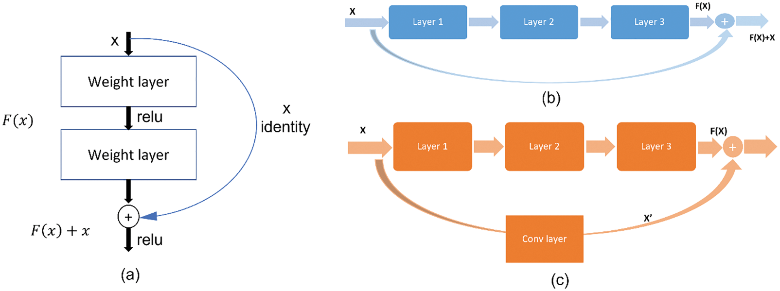
Figure 2: (a) Residual block (b) Identity block (c) Convolution block

The approach includes that instead of underlying mapping learned by the layers, we allow residual mapping to fit by the network. Consider H(x) as the underlying mapping that will be fit by several layers with x as input. So instead of initial mapping, H(x), let the network fit an approximate residual function as F(x):=H(x)−x so that the original function then becomes as H(x):=F(x)+x.

Two types of skip connections are used in residual networks which are identity and convolution blocks. The identity block is the standard block and is used when dimensions are the same for input and output activations. It directly adds the residue to the output as shown in Fig. 2b.

Convolution block corresponds to the case when the dimensions of input and output don’t match up. It performs convolution followed by batch normalization on the residue before adding it to the output as shown in Fig. 2c. Residual network architecture consists of seventeen convolution layers, a single fully connected and SoftMax layer. It uses a 3×3 filter with 1 as pad as well as stride and the average pooling layer consists of a 1×1 filter.

Fig. 3 presents the DSRNN architecture used in our proposed method. We first detail the training process on LR-residual image pairs and then extend to its corresponding subbands based on SVD. The network input is an LR image that has been down sampled using bicubic interpolation from the HR image. Let L and H denote the interpolated LR and corresponding HR image respectively. The network trains a model that predicts the residual images based on LR training examples. The main objective of the residual network is, rather than estimating HR images directly, it estimates the difference between the input and output images known as residue R and R=H−L. The residual images are desired responses from the network.

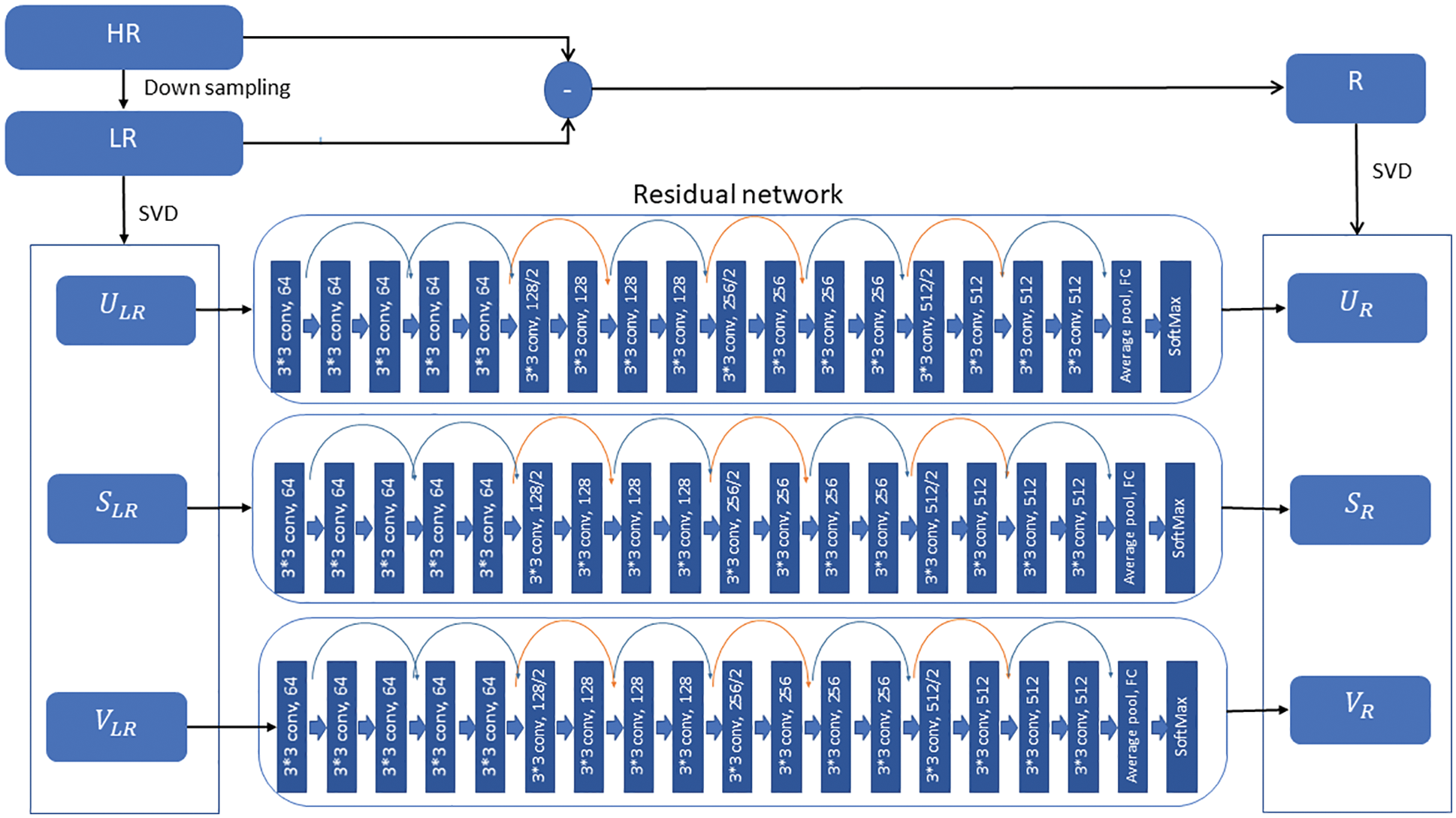
Figure 3: Proposed DSRNN architecture

During training data augmentation is used to vary training data, which increases the training data amount available. Random patch extraction is performed from the datastores of residual and up sampled images. It involves the extraction of small image tiles or patches as a huge set from a single large image in the training set, significantly increasing the training set size.

The loss function is represented as 12‖R−k(L)‖22. The biases and weights are determined by optimizing this function and to achieve the network optimum parameters, the stochastic gradient descent with momentum (SGDM) technique was used. In our work, the residual network is trained on the SVD subbands of numerous LR-HR examples and the obtained parameters are employed in the testing phase.

2.3 Proposed Method

The proposed methodology is depicted in the form of a block diagram as shown in Fig. 4. Our workflow majorly involves LR preprocessing using SVD, residual approximation with DSRNN followed by SR reconstruction.

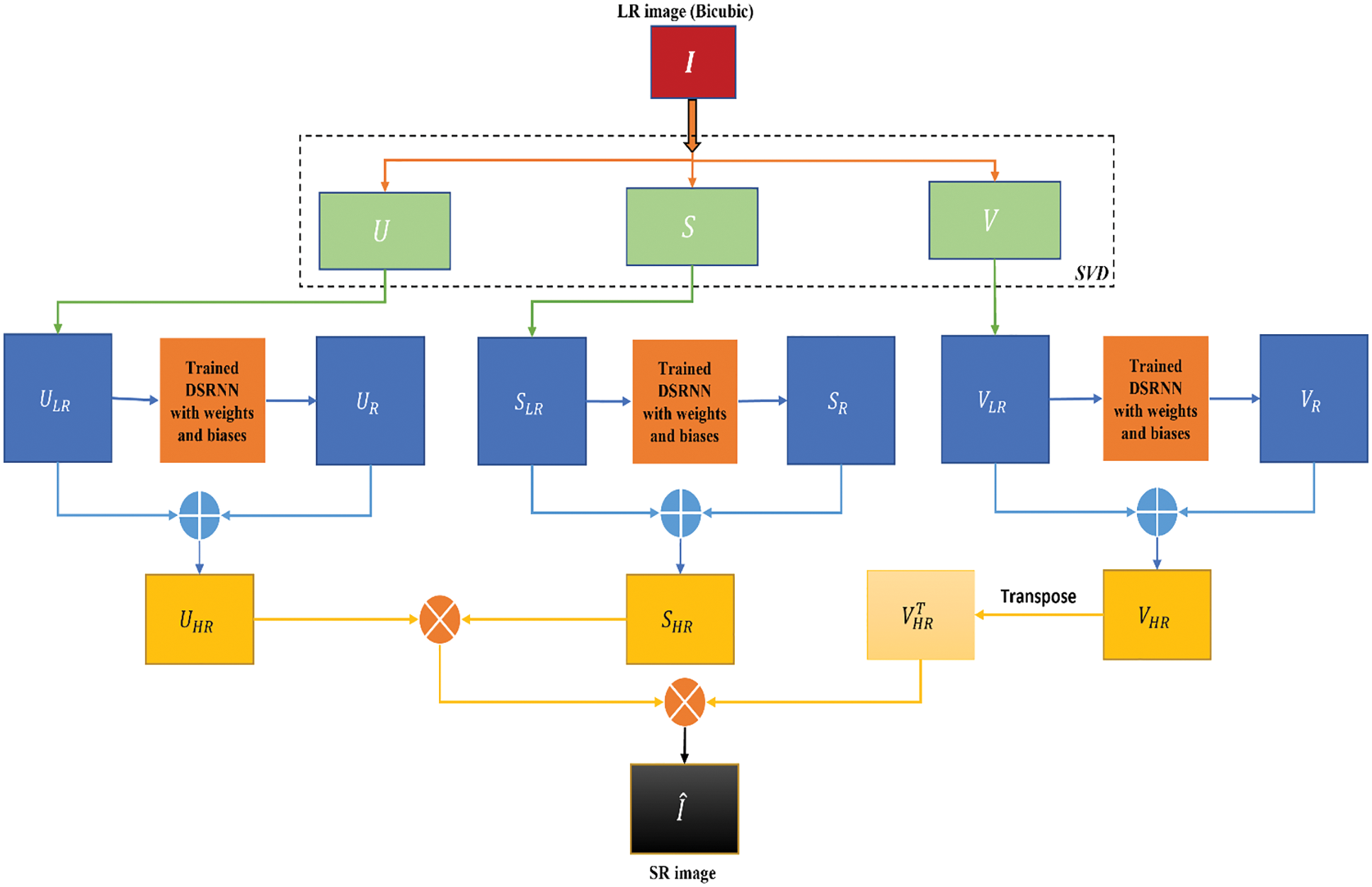
Figure 4: Proposed SR method block diagram

SVD is performed to decompose the given LR input into low and high frequency components. For an LR image input I, SVD involves factorization into three sub-matrices consisting of right singular vectors (U), singular values (S), and left singular vectors (V). The decomposed LR subbands are represented as ULR, SLR and VLR. Singular values are stored in SLR which represents the intensity information of an image. DSRNN uses skip connections which reduces the accuracy saturation problem and results in less training error. As the network consists of a few layers, the speed of the training accelerates by effectively reducing the vanishing gradient problem. Obtained LR subbands are given as inputs to the DSRNN with tuned weights and biases. DSRNN yields better generalization properties by avoiding overfitting. It transforms each LR subband input into desired residual outputs represented as UR, SR and VR.

These residuals consist of high frequency information which is used to recover the LR image. Adding each LR subband with the corresponding residual subband yields the HR subbands UHR, SHR and VHR as given in Eqs. (2)–(4).

UHR=ULR+UR,(2)

SHR=SLR+SR(3)

VHR=VLR+VR,(4)

Finally, inverse SVD is applied on these resultant HR subbands to produce the final SR image as

I^=UHRSHRVHRT(5)

Here VHRT represents the transpose of the subband VHR. The SR image, I^ has enhanced edge details with reduced blurring.

3  Results and Discussion

This section is dedicated to performing experiments to analyze the effectiveness of our method. We detailed the image datasets and compare outcomes with different methods and metrics. Finally, the results are analyzed through visual quality and quantitative assessments.

3.1 Image Datasets

The training dataset for DSRNN is a publicly available IAPRTC-12 dataset [25]. This benchmark image collection includes 20000 natural images from various parts of the world, representing various still image fragments. It consists of images of various sports and activities, people, cities, animals, landscapes, and many aspects of modern life. A small subset of 616 images from the IAPRTC-12 benchmark is used to train the network. Each image is down sampled with factor 4 using bicubic interpolation to produce LR images as network inputs and residual images are the desired responses of the network that are derived from the difference between the HR and LR images.

Test datasets include three popular benchmark datasets namely set5 which consists of 5 images, set14 consists of 14 images and urban100 consists of 100 images. The outcomes of various methods on these test datasets are discussed in the following sections.

3.2 Parameter Settings

In the training phase, to generate pairs of LR-HR images, a scaling factor of 4 is applied to downscale HR images. SVD decomposes LR images into {ULR, SLR, VLR} subbands and HR images into {UHR, SHR, VHR} subbands. LR subbands are subtracted from the HR subbands to generate residuals {UR, SR, VR}. The DSRNN is trained upon each LR subband and its corresponding residual subband pairs. The depth of the network is 20 and batches of 64 sizes are used in training. Momentum and weight decay parameters are set to 0.9 and 0.0001 respectively. Initially, the learning rate is set to 0.1, and for every 20 epochs, it is decreased by a factor of 10.

In the testing phase, ground truth images of size sm×sn from set5, set14, and urban100 are considered. Bicubic interpolation is performed to down sample to LR images of size m×n and upscale these images by the same factor s = 4. Bicubic upscaled images of size sm×sn are also considered LR images. We use SVD for subband decomposition and each subband passed through trained DSRNN with updated weights and biases to generate the residual subband. The addition of these residuals with LR subbands generates corresponding HR subbands {UHR, SHR, VHR}. Finally, the resultant SR image output of size sm×sn is obtained by the application of inverse SVD on {UHR,SHR,VHRT}. VHRT represents the transposed version of VHR.

3.3 Methods and Metrics

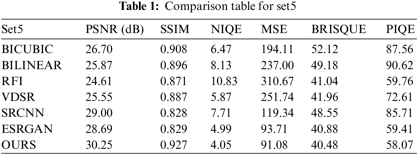
This section involves a comparison with traditional approaches such as bilinear, bicubic and popular methods such as rational fractal interpolation (RFI), SRCNN, VDSR, and ESRGAN. To evaluate the effectiveness of the methods, reference objective assessment indices such as peak signal-to-noise ratio (PSNR), mean squared error (MSE), structural similarity index (SSIM), and non-reference-based indices such as perception-based image quality evaluator (PIQE), natural image quality evaluator (NIQE), blind or reference-less image spatial quality evaluator (BRISQUE) are used.

PSNR is the ratio of the maximum possible performance of a given image to the performance of disturbing noise affecting the quality. SSIM motive is to quantify image degradation due to processing such as losses in data transmission or by data compression. NIQE is a quality analyzer of a blind image that uses deviations from the statistical patterns observed in images without human distorted image training and distortion. However, there is almost no exposure to the image. The total squared error between compressed and original images is MSE. BRISQUE compares the image to a primary image of a natural scene with similar distortion. The PIQE is a reference less image quality score that is inversely proportional to perceived image quality. For the system to be effective, it is desired to have high PSNR and SSM values and lower NIQE, MSE, BRISQUE and PIQE values.

3.4 Qualitative and Quantitative Assessment

Figs. 5a–11a represents the LR images, the interpolation results of bilinear and bicubic are shown in Figs. 5b–11b and Figs. 5c–11c. Figs. 5d–11d shows the results of RFI and Figs. 5e–11e, Figs. 5f–11f, Figs. 5g–11g represent deep learning methods SRCNN, VDSR, ESRGAN. Finally, Figs. 5h–11h depicts the results of our proposed method. As we can analyze from the reconstructed SR images of various methods in Figs. 6–11, the resultant SR image of the proposed method is more natural to human perception. However, the SR images of bilinear, bicubic and RFI contain ringing and blurred artifacts, and the salient features are not well restored. The deep learning methods have images with a minimal number of artifacts and reduced distortion, but the exact information is not clear either. When compared to other reconstruction approaches, the proposed method preserves structural and detailed information well and contains more prominent features for all the examples, and achieves better performance.

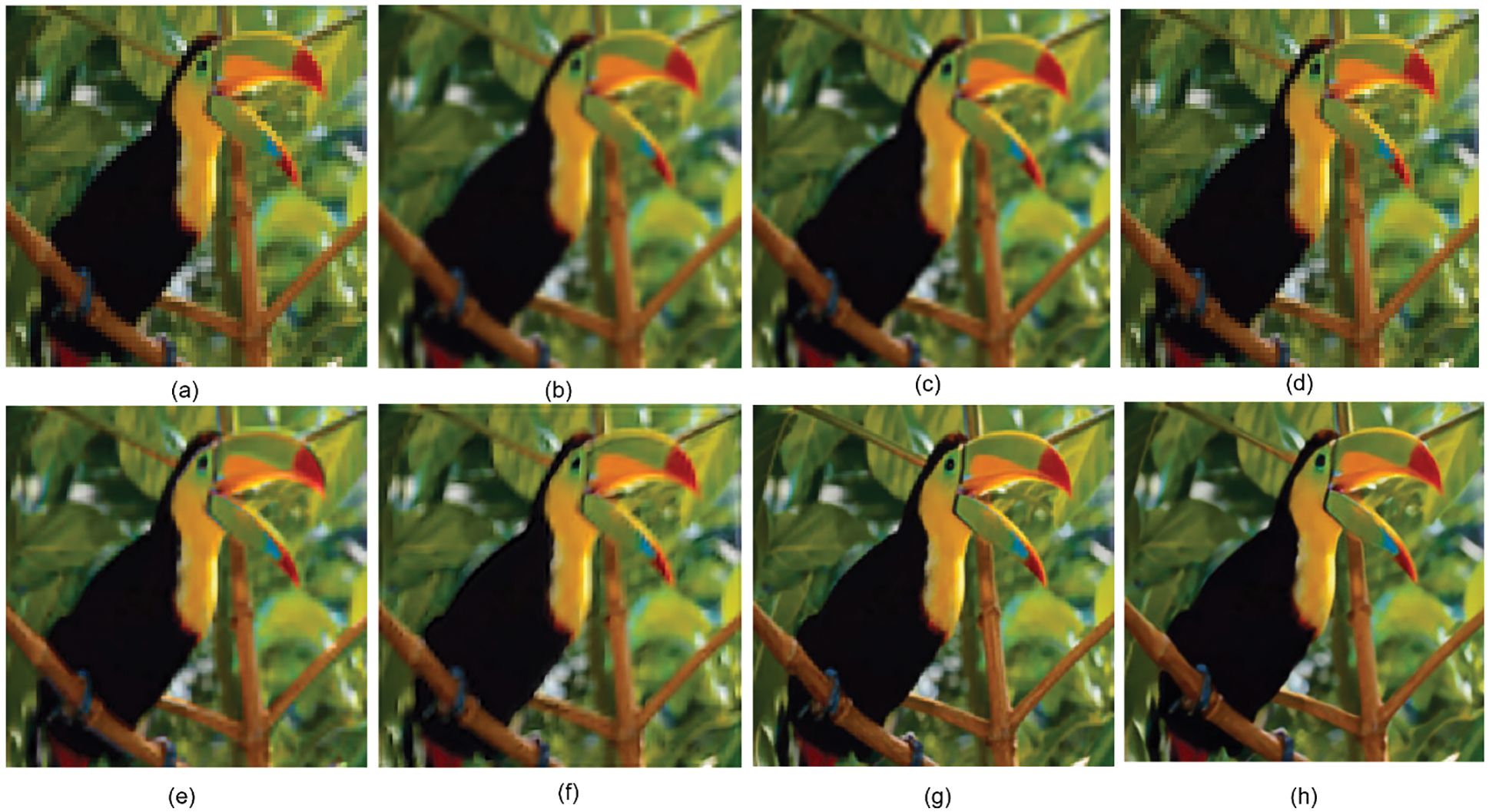
Figure 5: SR outcomes on bird image: (a) LR image (b) Bilinear (c) Bicubic (d) RFI (e) SRCNN (f) VDSR (g) ESRGAN (h) Proposed

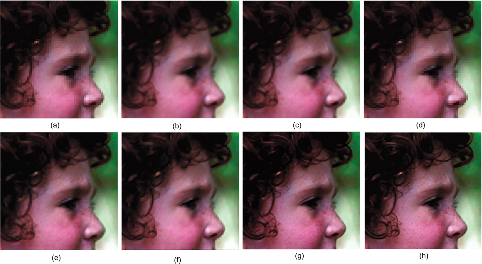
Figure 6: SR outcomes on head image: (a) LR image (b) Bilinear (c) Bicubic (d) RFI (e) SRCNN (f) VDSR (g) ESRGAN (h) Proposed

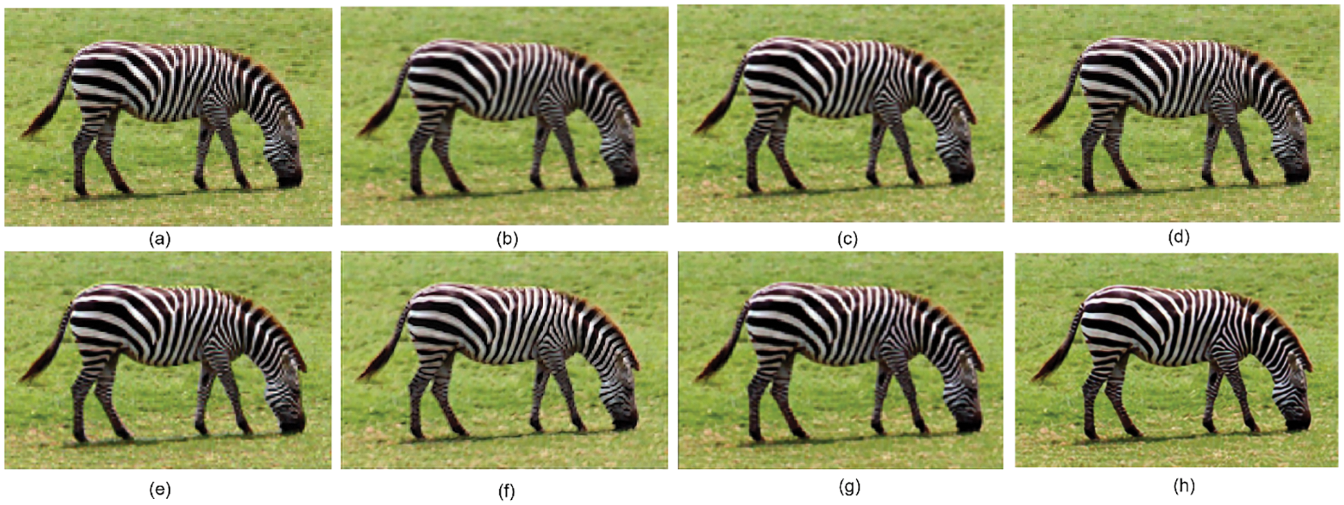
Figure 7: SR outcomes on zebra image: (a) LR image (b) Bilinear (c) Bicubic (d) RFI (e) SRCNN (f) VDSR (g) ESRGAN (h) Proposed

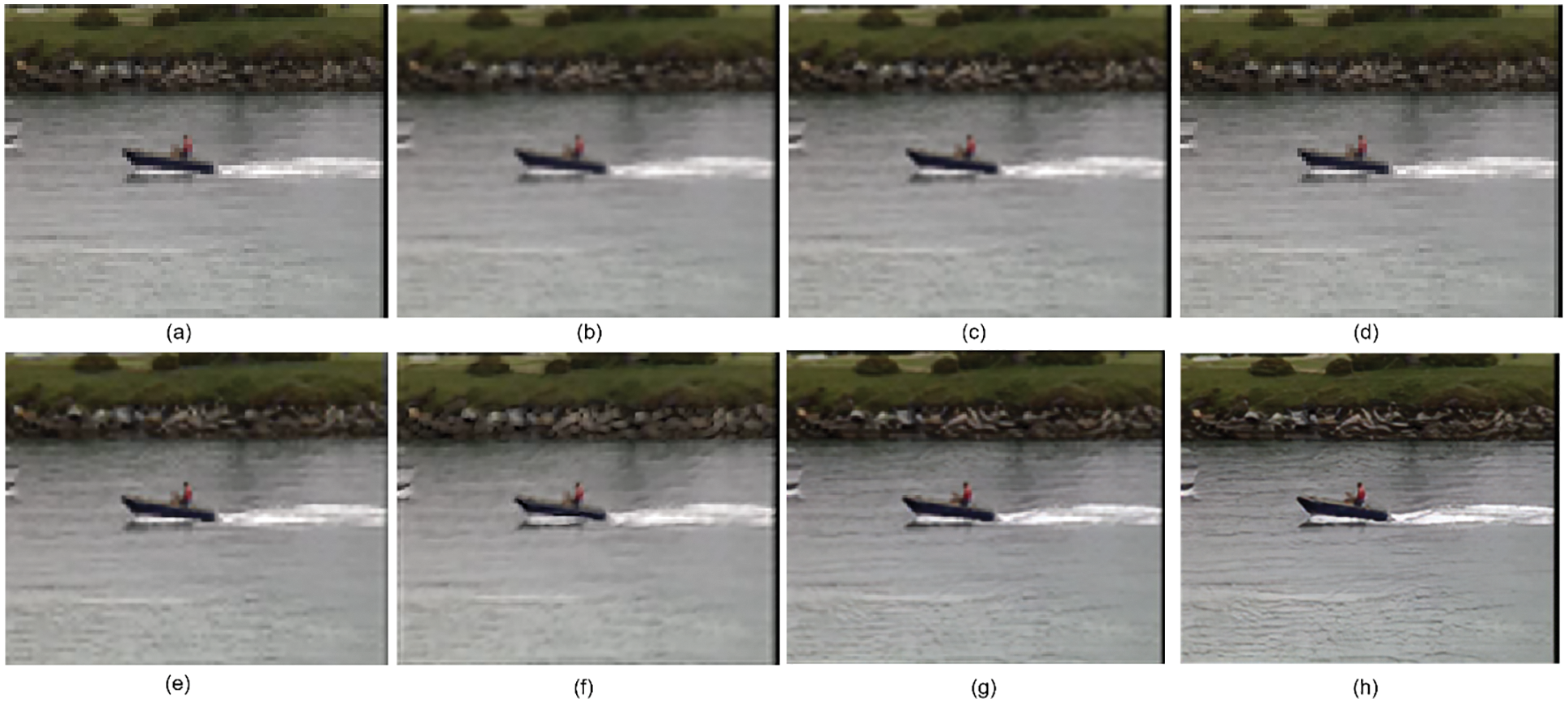
Figure 8: SR outcomes on coastguard image: (a) LR image (b) Bilinear (c) Bicubic (d) RFI (e) SRCNN (f) VDSR (g) ESRGAN (h) Proposed

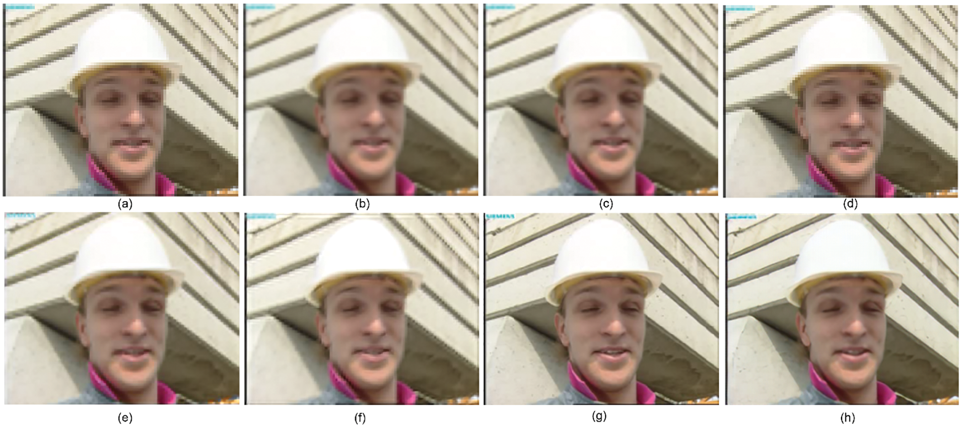
Figure 9: SR outcomes on foreman image: (a) LR image (b) Bilinear (c) Bicubic (d) RFI (e) SRCNN (f) VDSR (g) ESRGAN (h) Proposed

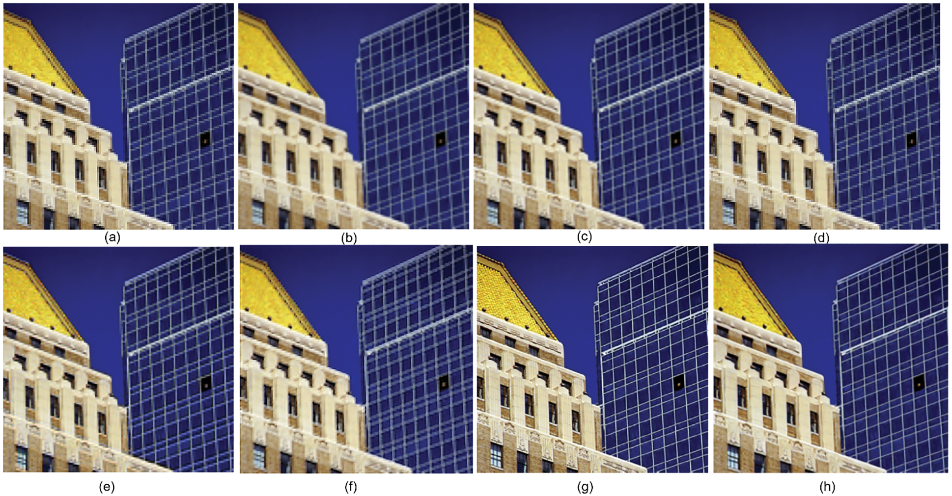
Figure 10: SR outcomes on urban image: (a) LR image (b) Bilinear (c) Bicubic (d) RFI (e) SRCNN (f) VDSR (g) ESRGAN (h) Proposed

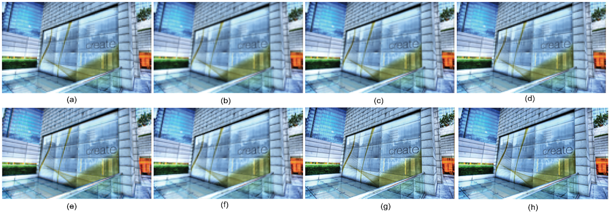
Figure 11: SR outcomes on urban image: (a) LR image (b) Bilinear (c) Bicubic (d) RFI (e) SRCNN (f) VDSR (g) ESRGAN (h) Proposed

To assess the reconstruction performance, six quantitative indicators described above are utilized. Tab. 1 presents the PSNR, SSIM, NIQE, MSE, BRISQUE, PIQE metrics for set5 images. Each metric value represents the average value of all five images from the set5. It is observable that the proposed method delivered better results across all the metrics and outperformed all the other methods. Although deep learning methods have shown comparable results, ESRGAN has shown better performance in NIQE, MSE, BRISQUE, and PIQE. However, it can also be noticed that RFI yields poor results in terms of PSNR, SSIM, and NIQE. Traditional methods such as bilinear and bicubic produced poor results in BRISQUE and PIQE metrics.

Tabs. 2 and 3 represent the quantitative comparison tables for set14 and urban100 images. Each value in Tab. 2 of the metrics was obtained from the average values of all 14 images. For Tab. 3, a subset of the urban100 dataset consisting of seven images is taken and each metric value represents the average values of all 7 images. It can be observed that RFI achieved poor results in terms of PSNR, NIQE, and MSE values. Bilinear and bicubic contain poor results in BRISQUE and PIQE metrics. From all three tables, it is evident that the proposed approach outshines other methods and has better reconstruction performance than other compared methods. For better visual interpretation, we have represented the average metric indices over set5, set14, and urban datasets as statistical graphs in Fig. 12.

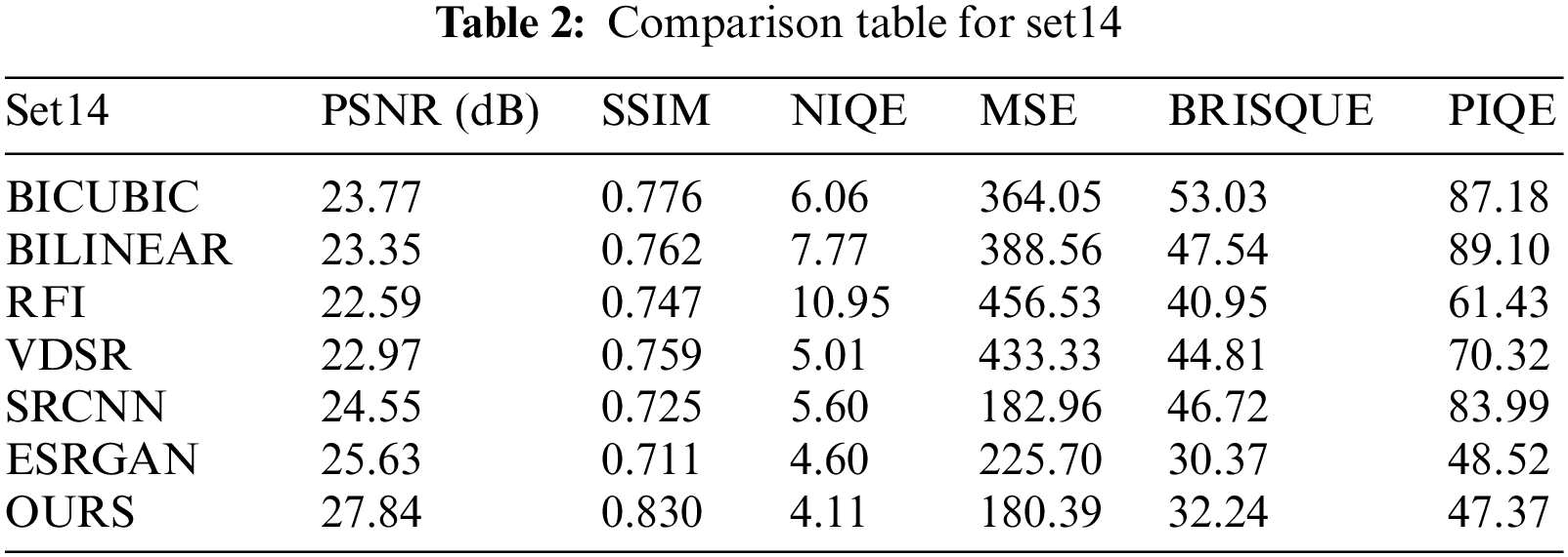
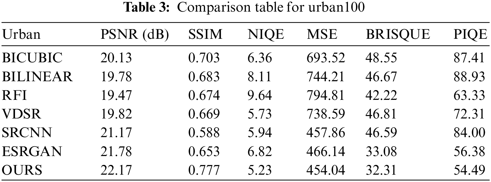
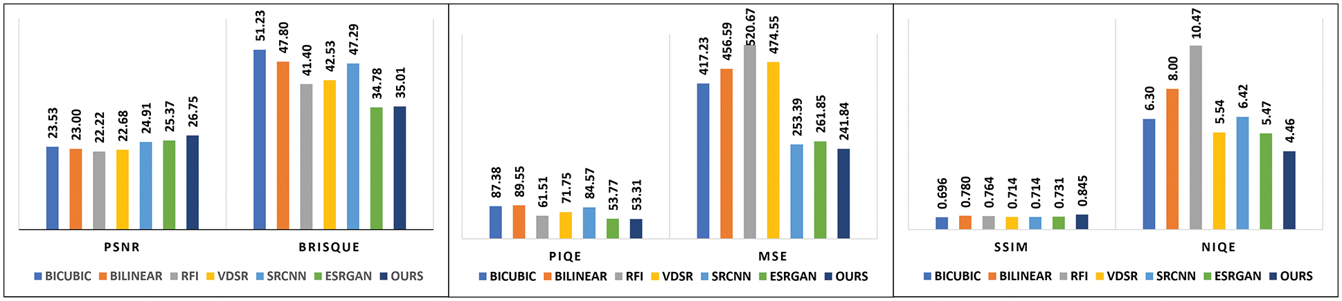
Figure 12: Average metric indices of different methods

4  Conclusion

This paper introduces a deep learning framework with DSRNN for SR reconstruction. With SVD, we achieve optimal low-rank approximations of the input images and a better understanding of n-space geometry. While learning the LR-residual pairs, the DSRNN quickly brings down the error rate to an appropriate level resulting in reduced computational complexity. The learned residuals effectively recover the lost high frequency information in the testing phase on set5, set14, and urban100 image datasets. The effectiveness of the proposed approach over other SR approaches can be noticed in terms of subjective analysis and objective metrics. We noticed that the proposed method has a maximum average improvement of 4.53 dB over RFI and a minimum of 1.38 dB over ESRGAN in terms of PSNR. Similarly, NIQE of our method overperforms RFI and ESRGAN methods with an improvement of 6.07 and 1.01 respectively.

Funding Statement: The authors received no specific funding for this study.

Conflicts of Interest: The authors declare that they have no conflicts of interest to report regarding the present work.

References

1. S. C. Park, M. K. Park and M. G. Kang, “Super-resolution image reconstruction: A technical overview,” IEEE Signal Processing Magazine, vol. 20, no. 3, pp. 21–36, 2003. [Google Scholar]
2. G. Suryanarayana, K. Chandran, O. I. Khalaf, Y. Alotaibi, A. Alsufyani et al., “Accurate magnetic resonance image super-resolution using deep networks and Gaussian filtering in the stationary wavelet domain,” IEEE Access, vol. 9, pp. 71406–71417, 2021. [Google Scholar]
3. K. Sathya and M. Rajalakshmi, “Enhanced super resolution method for rice plant disease classification,” Computer Systems Science and Engineering, vol. 42, no. 1, pp. 33–47, 2022. [Google Scholar]
4. T. Yang, “Research on the application of super resolution reconstruction algorithm for underwater image,” Computers, Materials & Continua, vol. 62, no. 3, pp. 1249–1258, 2020. [Google Scholar]
5. F. Zhou, W. Yang and Q. Liao, “Interpolation-based image super-resolution using multisurface fitting,” IEEE Transactions on Image Processing, vol. 21, no. 7, pp. 3312–3318, 2012. [Google Scholar]
6. Y. Zhang, Q. Fan, F. Bao, Y. Liu and C. Zhang, “Single-image super-resolution based on rational fractal interpolation,” IEEE Transactions on Image Processing, vol. 27, no. 8, pp. 3782–3797, 2018. [Google Scholar]
7. K. Shao, Q. Fan, Y. Zhang, F. Bao and C. Zhang, “Noisy single image super-resolution based on local fractal feature analysis,” IEEE Access, vol. 9, pp. 33385–33395, 2021. [Google Scholar]
8. G. Suryanarayana and D. Ravindra, “Simultaneous edge preserving and noise mitigating image super-resolution algorithm,” AEU-International Journal of Electronics and Communications, vol. 70, no. 4, pp. 409–415, 2016. [Google Scholar]
9. G. Suryanarayana and R. Dhuli, “Image resolution enhancement using wavelet domain transformation and sparse signal representation,” Procedia Computer Science, vol. 92, pp. 311–316, 2016. [Google Scholar]
10. G. Suryanarayana, R. Dhuli and J. Yang, “Single image super-resolution algorithm possessing edge and contrast preservation,” International Journal of Image and Graphics, vol. 19, no. 4, pp. 1950024, 2019. [Google Scholar]
11. S. Farsiu, M. D. Robinson, M. Elad and P. Milanfar, “Fast and robust multiframe super resolution,” IEEE Transactions on Image Processing, vol. 13, no. 10, pp. 1327–1344, 2004. [Google Scholar]
12. D. H. Trinh, M. Luong, F. Dibos, J. M. Rocchisani, C. D. Pham et al., “Novel example-based method for super-resolution and denoising of medical images,” IEEE Transactions on Image Processing, vol. 23, no. 4, pp. 1882–1895, 2014. [Google Scholar]
13. S. Farsiu, M. D. Robinson, M. Elad and P. Milanfar, “Fast and robust multiframe super resolution,” IEEE Transactions on Image Processing, vol. 13, no. 10, pp. 1327–1344, 2004. [Google Scholar]
14. G. Suryanarayana and R. Dhuli, “Sparse representation based super-resolution algorithm using wavelet domain interpolation and nonlocal means,” TELKOMNIKA Indonesian Journal of Electrical Engineering, vol. 16, no. 2, pp. 296–302, 2015. [Google Scholar]
15. N. Y. Arbel, A. Tal and L. Zelnik-Manor, “Partial correspondence of 3D shapes using properties of the nearest-neighbor field,” Computers & Graphics, vol. 82, pp. 183–192, 2019. [Google Scholar]
16. S. Yu, W. Kang, S. Ko and J. Paik, “Single image super-resolution using locally adaptive multiple linear regression,” JOSA A, vol. 32, no. 12, pp. 2264–2275, 2015. [Google Scholar]
17. C. Dong, C. C. Loy, K. He and X. Tang, “Image super-resolution using deep convolutional networks,” IEEE Transactions on Pattern Analysis and Machine Intelligence, vol. 38, no. 2, pp. 295–307, 2015. [Google Scholar]
18. P. Yadlapalli, D. Bhavana and S. Gunnam, “Intelligent classification of lung malignancies using deep learning techniques,” International Journal of Intelligent Computing and Cybernetics, vol. 24, no. 5, pp. 1038, 2021. [Google Scholar]
19. G. Suryanarayana, K. N. Rajesh and J. Yang, “Super-resolution based on residual learning and optimized phase stretch transform,” International Journal of Image and Graphics, vol. 21, no. 1, pp. 2150008, 2021. [Google Scholar]
20. G. R. Hemalakshmi, D. Santhi, V. R. S. Mani, A. Geetha and N. B. Prakash, “Deep residual network based on image priors for single image super resolution in FFA images,” Computer Modeling in Engineering & Sciences, vol. 125, no. 1, pp. 125–143, 2020. [Google Scholar]
21. V. Romanuke, “An improvement of the VDSR network for single image super-resolution by truncation and adjustment of the learning rate parameters,” Applied Computer Systems, vol. 24, no. 1, pp. 61–68, 2019. [Google Scholar]
22. A. K. Cherian and E. Poovammal, “A novel AlphaSRGAN for underwater image super resolution,” CMC-Computers Materials & Continua, vol. 69, no. 2, pp. 1537–1552, 2021. [Google Scholar]
23. G. Suryanarayana and R. Dhuli, “Super-resolution image reconstruction using dual-mode complex diffusion-based shock filter and singular value decomposition,” Circuits, Systems, and Signal Processing, vol. 36, no. 8, pp. 3409–3425, 2017. [Google Scholar]
24. G. Suryanarayana, E. Tu and J. Yang, “Infrared super-resolution imaging using multi-scale saliency and deep wavelet residuals,” Infrared Physics & Technology, vol. 97, pp. 177–186, 2019. [Google Scholar]
25. S. Zhu, Z. Shi, C. Sun and S. Shen, “Deep neural network based image annotation,” Pattern Recognition Letters, vol. 65, pp. 103–108, 2015. [Google Scholar]
26. D. Zhang, J. Hu, F. Li, X. Ding, A. K. Sangaiah et al., “Small object detection via precise region-based fully convolutional networks,” Computers, Materials & Continua, vol. 69, no. 2, pp. 1503–1517, 2021. [Google Scholar]
27. J. Wang, Y. Wu, S. He, P. K. Sharma, X. Yu et al., “Lightweight single image super-resolution convolution neural network in portable device,” KSII Transactions on Internet and Information Systems (TIIS), vol. 15, no. 11, pp. 4065–4083, 2021. [Google Scholar]
28. J. Wang, Y. Zou, P. Lei, R. S. Sherratt and L. Wang, “Research on recurrent neural network based crack opening prediction of concrete dam,” Journal of Internet Technology, vol. 21, no. 4, pp. 1161–1169, 2020. [Google Scholar]
29. J. Zhang, J. Sun, J. Wang and X. G. Yue, “Visual object tracking based on residual network and cascaded correlation filters,” Journal of Ambient Intelligence and Humanized Computing, vol. 12, no. 8, pp. 8427–8440, 2021. [Google Scholar]
30. S. He, Z. Li, Y. Tang, Z. Liao, F. Li et al., “Parameters compressing in deep learning,” Computers, Materials & Continua, vol. 62, no. 1, pp. 321–336, 2020. [Google Scholar]
31. S. R. Zhou and B. Tan, “Electrocardiogram soft computing using hybrid deep learning CNN-ELM,” Applied Soft Computing, vol. 86, pp. 105778, 2020. [Google Scholar]
32. S. R. Zhou, M. L. Ke and P. Luo, “Multi-camera transfer GAN for person re-identification,” Journal of Visual Communication and Image Representation, vol. 59, no. 1, pp. 393–400, 2019. [Google Scholar]
33. W. Wang, H. Liu, J. Li, H. Nie and X. Wang, “Using CFW-net deep learning models for X-ray images to detect COVID-19 patients,” International Journal of Computational Intelligence Systems, vol. 14, no. 1, pp. 199–207, 2021. [Google Scholar]
34. W. Wang, Y. Jiang, Y. Luo, J. Li, X. Wang et al., “An advanced deep residual dense network (DRDN) approach for image super-resolution,” International Journal of Computational Intelligence Systems, vol. 12, no. 2, pp. 1592–1601, 2019. [Google Scholar]
35. W. Wang, Y. Yang, J. Li, Y. Hu, Y. Luo et al., “Woodland labeling in chenzhou, China, via deep learning approach,” International Journal of Computational Intelligence Systems, vol. 13, no. 1, pp. 1393–1403, 2020. [Google Scholar]
36. W. Sun, X. Chen, X. R. Zhang, G. Z. Dai, P. S. Chang et al., “A multi-feature learning model with enhanced local attention for vehicle re-identification,” Computers, Materials & Continua, vol. 69, no. 3, pp. 3549–3560, 2021. [Google Scholar]
37. W. Sun, G. C. Zhang, X. R. Zhang, X. Zhang and N. N. Ge, “Fine-grained vehicle type classification using lightweight convolutional neural network with feature optimization and joint learning strategy,” Multimedia Tools and Applications, vol. 80, no. 20, pp. 30803–30816, 2021. [Google Scholar]
Cite This Article
Copyright © 2023 The Author(s). Published by Tech Science Press.
This work is licensed under a Creative Commons Attribution 4.0 International License , which permits unrestricted use, distribution, and reproduction in any medium, provided the original work is properly cited.
Downloads
Citation Tools