Distortion Evaluation of EMP Sensors Using Associated-Hermite Functions

1  Introduction

Electromagnetic pulse (EMP) is a kind of transient electromagnetic phenomenon. In the time domain, the rise time of the leading edge is short, and its spectrum is wide. Lightning, electrostatic discharge and high-power switch can produce electromagnetic pulse. EMP usually disrupts communications and damages electronic equipment and system by means of electromagnetic radiation and conduction.

EMP measurement is one of the important research topics in the damage and protection mechanism to the electronic equipment [1–5]. The measurement objects of EMP include electric field, magnetic field, voltage and current. According to this, the EMP sensors can be divided into electric field sensor, magnetic field sensor, voltage probe and current probe [6–9]. According to the different working principles of sensors, they can be divided into capacitive sensor and inductive sensor. Capacitive sensor is generally used to measure pulsed electric field and pulse voltage, while inductive sensor is generally used to measure pulsed magnetic field and pulse current. According to the different transfer characteristics of sensors, they can be divided into self-integrating sensor and differential sensor. The output of the self-integrating sensor has a linear relationship with the input, while the output of the differential sensor has a linear relationship with the time derivative of the input [10]. Due to the wide spectrum of EMP, it is difficult for a sensor or probe to realize undistorted measurement in the whole frequency band. Therefore, it is necessary to analyze the distortion of EMP measurement results in order to evaluate its distortion characteristics and compensate the measurement results. It is very important to select the appropriate distortion criterion for the study of distortion.

For ultra-wideband (UWB) antenna, waveform fidelity is an important index to measure antenna performance [11]. Fidelity is defined as the correlation coefficient between the received waveform and the excitation waveform [12]. On the other hand, the coefficient can also be used to judge the distortion of the received waveform relative to the excitation waveform. For broadband EMP measurement, the sensor and probe as the receiving antenna can also adopt the fidelity to analyze distortion. However, as the fidelity depends on the signal waveform, different input signals may get different fidelity values for the same sensor, which makes it difficult to comprehensively characterize the performance of a sensor [13]. The spectral element method (SEM) based on orthogonal basis shows superior accuracy in spatial electromagnetic calculation [14,15]. In time domain, distortion analysis based on Hermite-Gauss orthogonal basis function has been developed, which overcomes some of the mentioned fidelity drawbacks [16]. The distortion characteristics of the sensor can be calculated by a set of time-domain measurement values. In this paper, a novel distortion evaluation method is proposed based on the associated-hermite (AH) basis function. A new distortion rate is also defined, which is convenient for quantitative comparison of distortion. The range of distortion rate is 0∼1, the smaller the value, the smaller the sensor distortion, and vice versa. The results show that the proposed method is able to avoid the dependence of input waveform on the distortion analysis of EMP sensor; the system transfer matrix can directly reveal the distortion at different frequencies; the distortion rate facilitates quantitative calculation and comparative analysis of the distortion characteristics of different sensors.

2  Associated-Hermite Basis Function

The AH basis function is [17,18]

ϕn(t,σ)=1n!2nσπe−12(t−t0σ)2Hn(t−t0σ)(1)

where, n is the order of the AH basis function, σ is the scale factor, and t0 is the time shift factor.

Hn(t) is a Hermite polynomial of order n, which can be recursively defined as follows:

H0′(x)=0Hn′(x)=2nHn−1(x),n=1,2,⋯H0(x)=1H1(x)=2xH0(x)Hn+1(x)=2xHn(x)−2nHn−1(x),n=1,2,⋯(2)

Hermite polynomial Hn(x) is orthogonal to the weight function w(x)=e−x2 on (−∞,+∞)

∫−∞+∞e−x2Hm(x)Hn(x)¯dx={0,m≠n2nn!π,m=n(3)

Therefore, the AH basis function is the orthonormal basis

⟨ϕm(t,σ),ϕn(t,σ)⟩=∫−∞+∞ϕm(t,σ)ϕn(t,σ)¯dt={0,m≠n1,m=n(4)

As the AH basis function is the characteristic function of Fourier transform [19]. The frequency domain is expressed as [20]

F[ϕn(t,σ)]=(−i)n2πσϕn(ω,σ)(5)

It can be seen from the above formula that the shape of ϕn(t) function in frequency domain is similar to that in time domain.

The differential form of the AH basis function has the following relationship with the original function [20]

dϕn(x,σ)dx=n2σ2ϕn−1(x,σ)−n+12σ2ϕn+1(x,σ),n≥1(6)

When the AH basis function is used to analyze the signal, this property makes it convenient to analyze the characteristic relationship between the input and output of a signal system.

The scaling factor σ of the AH basis function is closely related to its support interval in the time domain and the frequency domain. If the time domain support interval of the AH basis function is Tn and the frequency domain support interval is Wn, then

Tnσ≈πn1.7+1.8(7)

Wn⋅σ≈πn1.7+1.82π(8)

The relationship between time domain support interval Tn and frequency domain support interval Wn of AH functions and its scaling factor σ and order n are shown in Fig. 1. When the order n is determined, the time-domain support interval Tn of the AH function increases with the scaling factor σ, and the frequency domain support interval Wn decreases with the increase of the scaling factor σ.

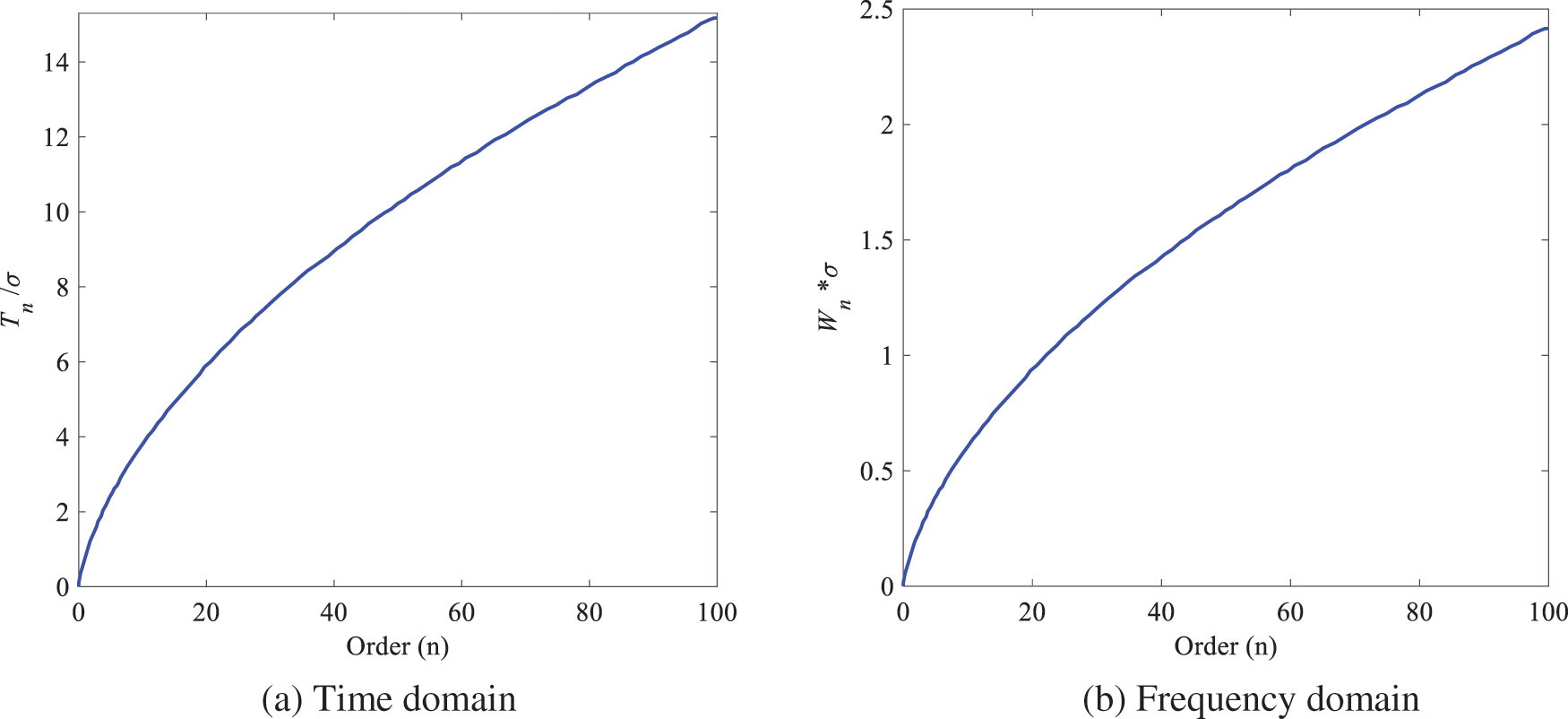
Figure 1: Time support and frequency support of AH functions with respect to σ and n

When the time period of the time domain signal f(t) is T and the frequency band width is W, and the AH basis function is used to express f(t), then

2Tn≥T(9)

Wn≥W(10)

Substituting formulas (7) and (8) into the above two formulas can be obtained

T2(πn1.7+1.8)≤σ≤πn1.7+1.82πW(11)

The time-domain support range of AH functions extends to both positive and negative sides with t=0 as the center. Therefore, the time shift factor t0 generally selects half of the signal duration, i.e., t0=T/2, which can reduce the order of AH functions.

3  System Transfer Matrix and Distortion Rate

The new definition of distortion rate is derived from the system transfer matrix represented by orthogonal basis functions. A system transfer function can be obtained by a time-domain measurement, and then the basis vector is taken as the excitation function and substituted into the transfer function to obtain N responses. Finally, the system transfer matrix can be obtained by calculating the coefficients of the N responses. The distortion rate can be obtained by comparing the system transfer matrix with the identity matrix.

3.1 System Transfer Matrix

An EMP signal with limited energy and certain pulse width belongs to the typical compactly support signal [19]. When the basis vector ϕn(t) is used for orthogonal decomposition of the EMP signal, the input signal e(t) and the output signal v(t) of the EMP sensor can be expressed as

e(t)=∑n=0N−1enϕn(t)(12)

v(t)=∑n=0N−1vnϕn(t)(13)

The coefficient of the basis vector can be expressed by the inner product as

en=⟨e(t),ϕn(t)⟩(14)

vn=⟨v(t),ϕn(t)⟩(15)

The input and output signals can be represented by the below vectors

e¯=[e1,e2,⋯,eN]t(16)

v¯=[v1,v2,⋯,vN]t(17)

where, t is the matrix transpose operator. The relation between the output voltage and the incident voltage can be expressed as the vector

v¯=Le¯(18)

where, L is the transition matrix, L=[lij]1≤i,j≤N.

According to formula (5), Fourier transform of Eqs. (12) and (13) can be obtained as

E(ω)=∑n=0N−1en(−i)n2πσϕn(ω,σ)(19)

V(ω)=∑n=0N−1vn(−i)n2πσϕn(ω,σ)(20)

Then, from Eqs. (19) and (20), the transfer function of the electromagnetic field sensor can be calculated as

H(ω)=∑n=0N−1vn(−i)nϕn(w,σ)∑n=0N−1en(−i)nϕn(w,σ)(21)

Since the Fourier transform form of the Associated-Hermite function is its characteristic function in the time domain, whose expressions in frequency domain and time domain have the same coefficients. In order to obtain the ijth element in the system transfer matrix, the Fourier expression of the basis vector ϕj−1(t) is substituted into Eq. (21)

Vj−1(ω)=H(ω)(−i)n2πσϕj−1(t,σ)(22)

The coefficient v¯j=[v¯0j,v¯1j,⋯,v¯N−1j]t of column j can be calculated by the following formula

v¯j=⟨Vj−1(ω),(−i)n2πσϕj−1(t,σ)⟩(23)

Then, the system transfer matrix is

L=[lij]=v¯ij,1≤i,j≤N(24)

For an ideal electromagnetic field sensor, the energy is normalized by the system transfer matrix as below

lijnorm=⟨ϕj−1(x),ϕi−1(x)⟩={1,j=i0,j≠i(25)

The absolute value graph of the corresponding system transition matrix is shown in Fig. 2a. i and j represent the rows and columns of the system transition matrix respectively. It is seen that only the main diagonal has values other than zero. For the ideal differential form sensor, the system transfer matrix is normalized to

lijnorm=⟨dϕj−1(t)dt,ϕi−1(t)⟩=⟨(j−12σ2ϕj−2(t,σ)−j2σ2ϕj(t,σ)),ϕi−1(t)⟩=⟨j−12σ2ϕj−2(t,σ),ϕi−1(t)⟩−⟨j2σ2ϕj(t,σ),ϕi−1(t)⟩={j−12σ2,j=i+1j2σ2,j=i−10,others(26)

The absolute value graph of the normalized system transfer matrix is shown in Fig. 2b. Only the sub-diagonal has values other than zero. This property of the system transfer matrix can be used to analyze system characteristics.

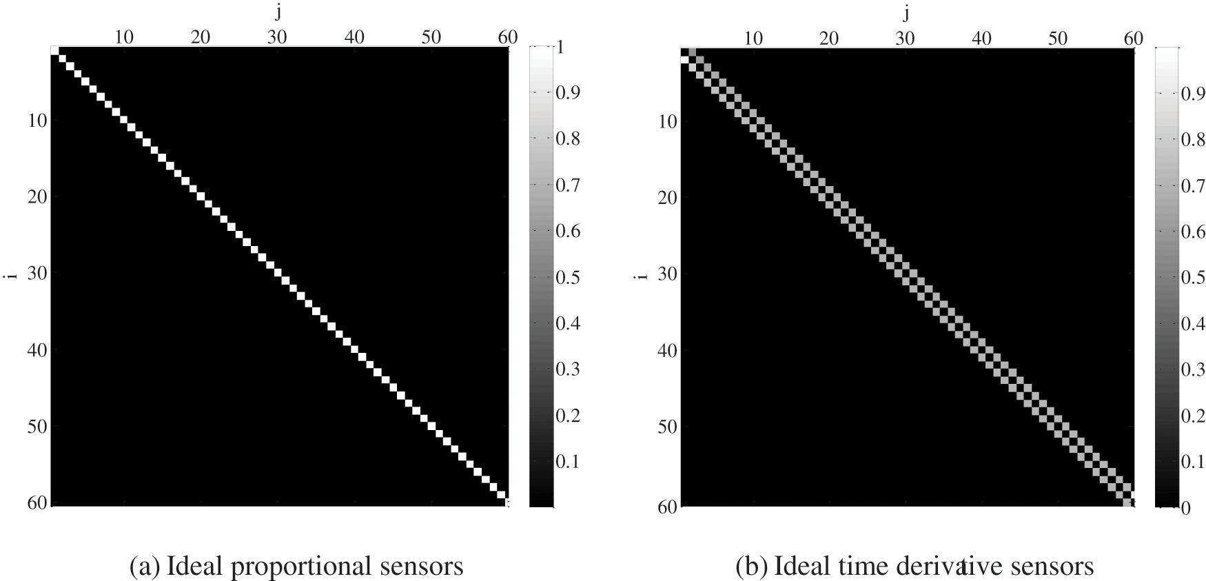
Figure 2: Absolute value of normalized system transfer matrix

3.2 Distortion Rate

When analyzing the distortion of a sensor, in order to do quantitative analysis, a distortion rate ηn is defined as [12]

ηn=‖Lnorm−I‖22n(27)

where, Lnorm is the system transfer matrix normalized to energy, I is the identity matrix, ‖⋅‖2 is Frobenius norm.

When calculating the distortion rate of differential sensor, the output waveform is usually integrated first, then the system transfer matrix is obtained by the Eq. (25) and substituted into the Eq. (27) to obtain the ηn. The value range of ηn is 0∼1. The smaller the value of ηn, the smaller the sensor distortion, and vice versa.

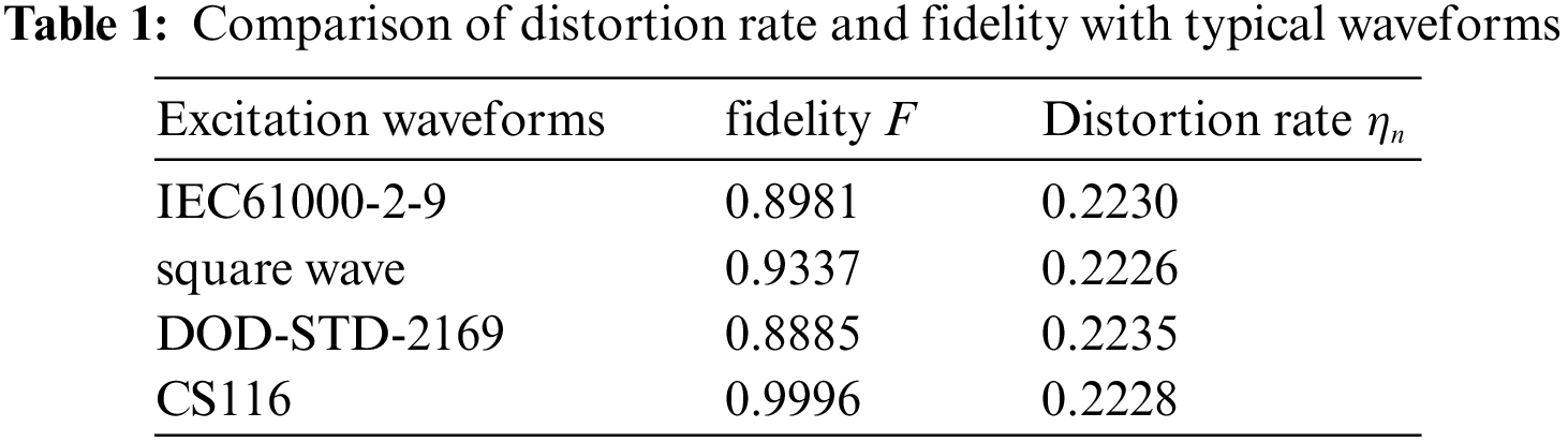
The distortion rate is different from the fidelity, and the calculation result no longer depends on the specific input waveform. Three-dimensional electromagnetic field computer simulation technology (CST) is employed to verity it by taking the inverted cone sensor as an example. The inverted cone sensor is placed in an electromagnetic environment formed by plane wave irradiation, and the load is a resistance and a capacitance in parallel. The simulation model is shown in Fig. 3. Several typical waveforms of high-altitude nuclear explosion electromagnetic pulse and electromagnetic compatibility are selected as excitation signals, as shown in Fig. 4a. Among them, IEC61000-2-9 waveform is the standard waveform of high-altitude electromagnetic pulse (HEMP) environmental radiation interference defined by the International Electrotechnical Commission, DOD-STD-2169 waveform is the military standard HEMP waveform formulated by the U.S. Department of defense, and CS116 waveform is the damped sinusoidal oscillation signal waveform used in China's military standard. Fig. 4b shows the corresponding output waveforms on the load of the inverted cone sensor. Because the sensor is of differential structure, these output waveforms are in differential form. The calculation results of distortion rate and fidelity are shown in Tab. 1. It can be seen from the table that when the excitation waveforms are different, the fidelities vary drastically, while the distortion rates are almost the same, which indicates that the distortion rate does not depend on the input waveform and can well characterize the transfer characteristics of a sensor.

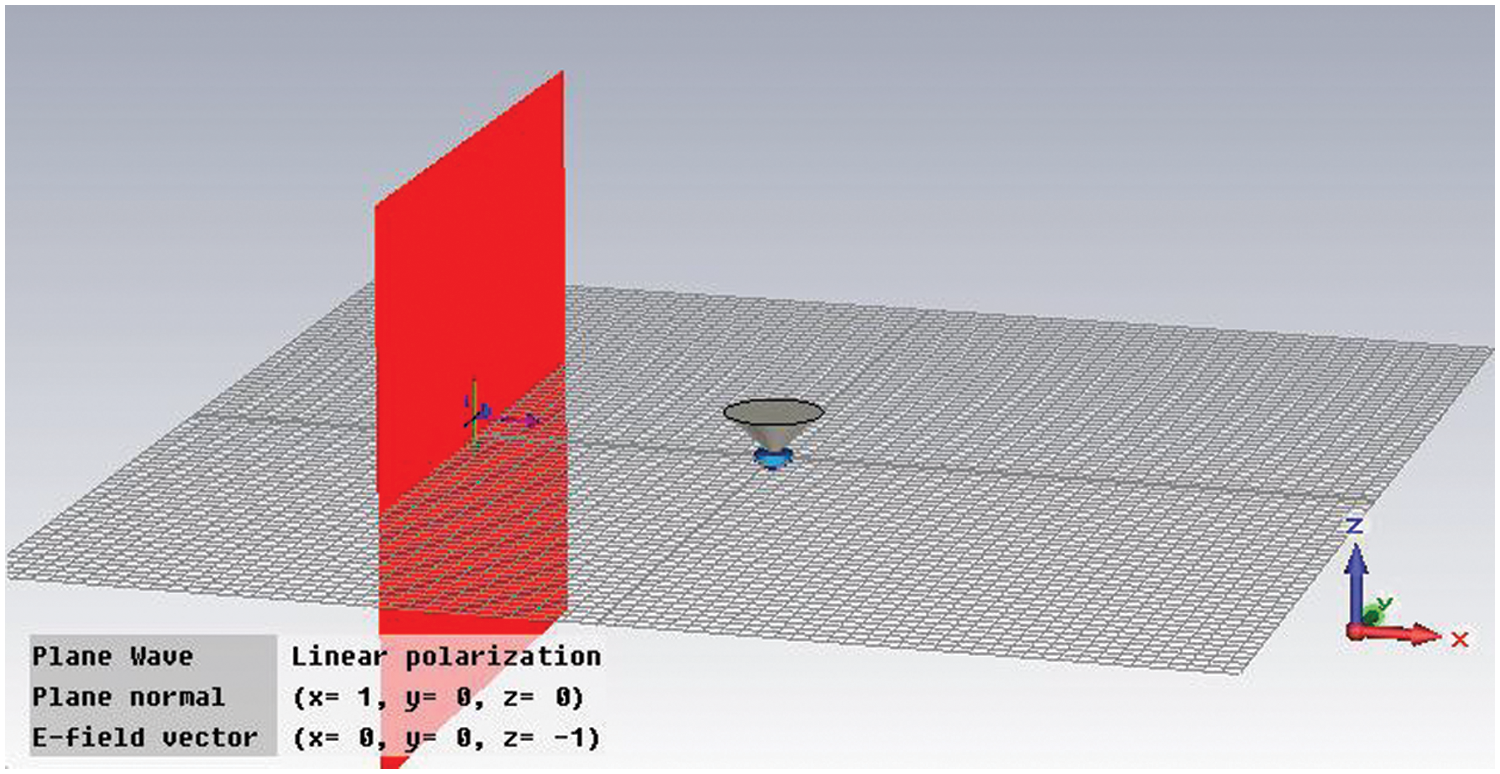
Figure 3: Simulation model of conical sensor

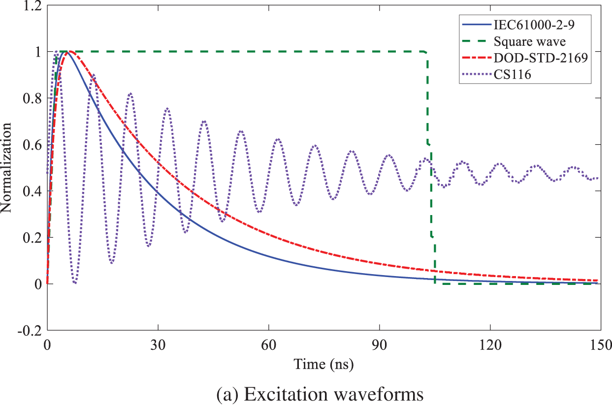
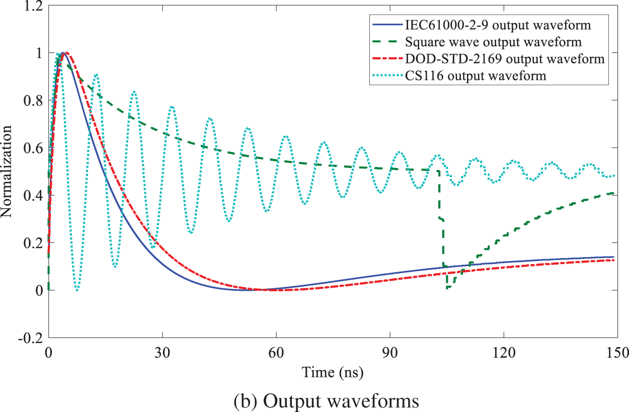
Figure 4: Normalized simulation waveforms of four typical waveforms

4  Distortion Analysis

Generally speaking, a signal is considered to be distorted when its output and input are nonlinear. For the differential sensor, its output is the differential form of the input, that is, obvious nonlinear distortion appears. In practical application, the output of the differential sensor is usually integrated, and the integrated waveform and input waveform will present a good linear relationship.

In order to verify the effect of distortion analysis based on the system transfer matrix and distortion rate based on AH functions, the waveforms measured by a current probe, a coaxial pulse voltage probe and a magnetic field sensor (also known as B sensor) are analyzed respectively.

The measured waveforms of the current probe, the coaxial pulse voltage probe and the B sensor are shown in Figs. 5–7, respectively. Because the input and output of the current probe are proportional, the coaxial pulse voltage probe is differential, and the B sensor has both. It can be seen from the figures that the output waveform of the current probe is basically consistent with the input waveform, the output waveform of the coaxial pulse voltage probe is the differential form of the input waveform, while the output waveform of B sensor has both proportional and differential forms.

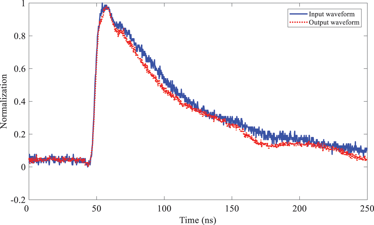
Figure 5: Input-output waveforms of the current probe

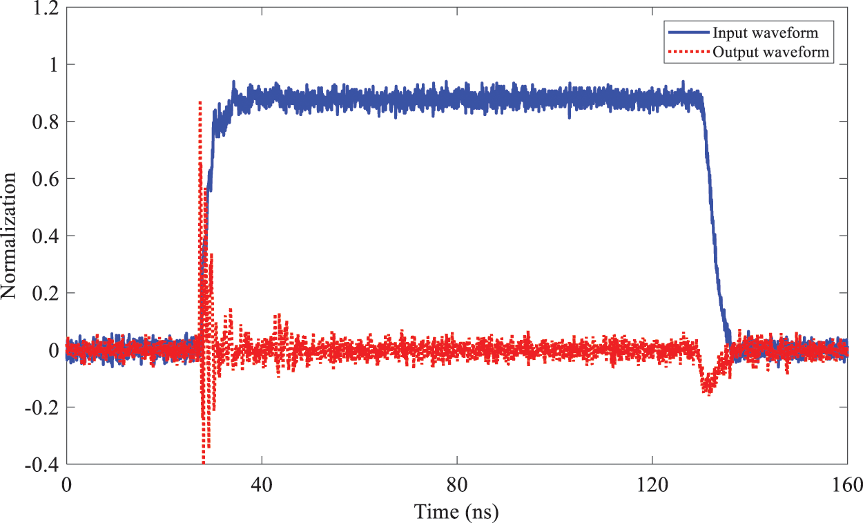
Figure 6: Input-output waveforms of the coaxial pulse voltage probe

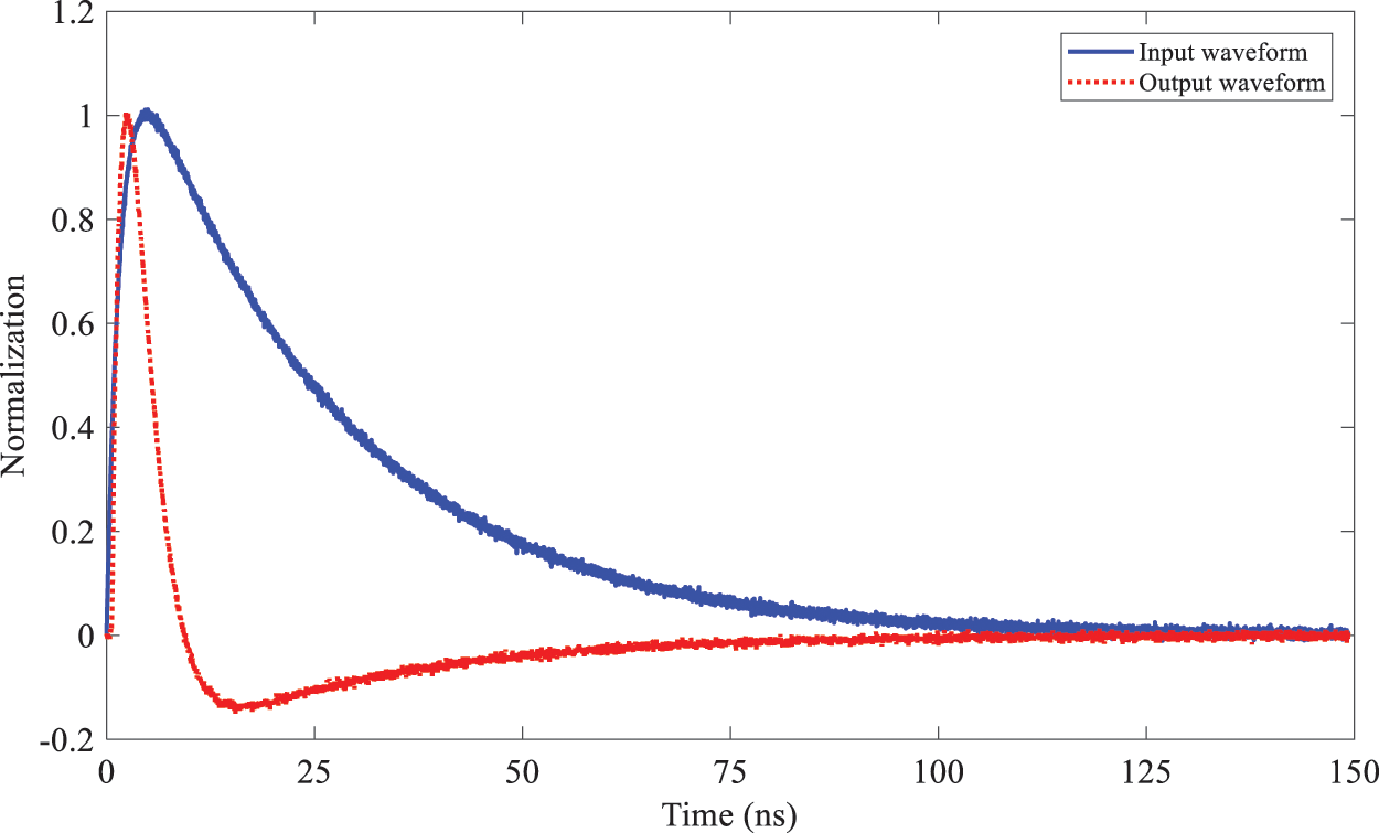
Figure 7: Input-output waveforms of the B sensor

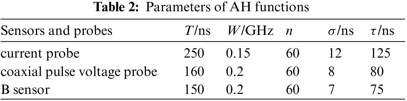
For the current probe, the frequency band width of the input waveform is W ≈ 0.15 GHz and the waveform period is T = 250 ns. Now take the maximum order n = 60, from formula (11), 10 ns ≤ σ ≤ 13 ns can be obtained,and σ = 12 ns is selected in this paper. Similarly, the values of scaling factor and the other parameters of the coaxial pulse voltage probe and the B sensor are shown in Tab. 2.

According to the calculation, the absolute value graph of the system transfer matrix of the current probe is shown in Fig. 8. The values of the system transfer matrix are mainly concentrated in the main diagonal position. The graph is similar to the system transfer matrix diagram of an ideal sensor. It is indicated that the input and output of the probe are proportional. Compared with Fig. 1b, the system transfer matrix shown in Fig. 8 begins to diverge after the 55th order, corresponding to a frequency of 0.15 GHz. Signals higher than this frequency are distorted.

Figure 8: Absolute value of normalized system transfer matrix for the current probe

The absolute value graph of the system transfer matrix of the coaxial pulse voltage probe is shown in Fig. 9. Fig. 9a shows the system transfer matrix calculated by the direct output of the probe. The value of the system transfer matrix is mainly concentrated in the sub diagonal position, which is similar to the system transfer matrix diagram of the ideal differential sensor. It is indicated that the coaxial pulse voltage probe is a differential probe. Fig. 9b shows the absolute value of the system transfer matrix calculated after integrating the output waveform. It can be seen that the integrated system transfer matrix diagram is similar to that of the ideal sensor. The divergence begins at the 50th order of the matrix, which corresponds to the frequency of 0.2 GHz. There is obvious distortion above the frequency.

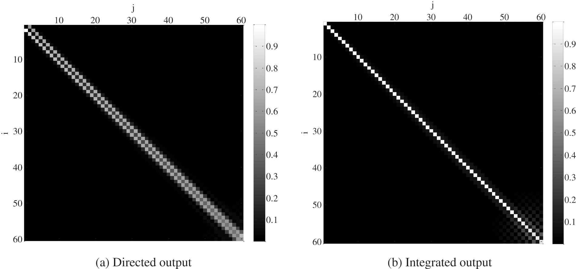
Figure 9: Absolute value of normalized system transfer matrix for the coaxial pulse voltage probe

The absolute value of the system transfer matrix of the B sensor is shown in Fig. 10. The value of the system transfer matrix is mainly concentrated in the sub diagonal position before the 15th order, and the main diagonal position after the 15th order, which is between the ideal sensor and the differential sensor. The corresponding frequency of the 15th order is 0.15 GHz. It is indicated that the input and output of the sensor have a differential relationship below the frequency and a linear relationship above the frequency.

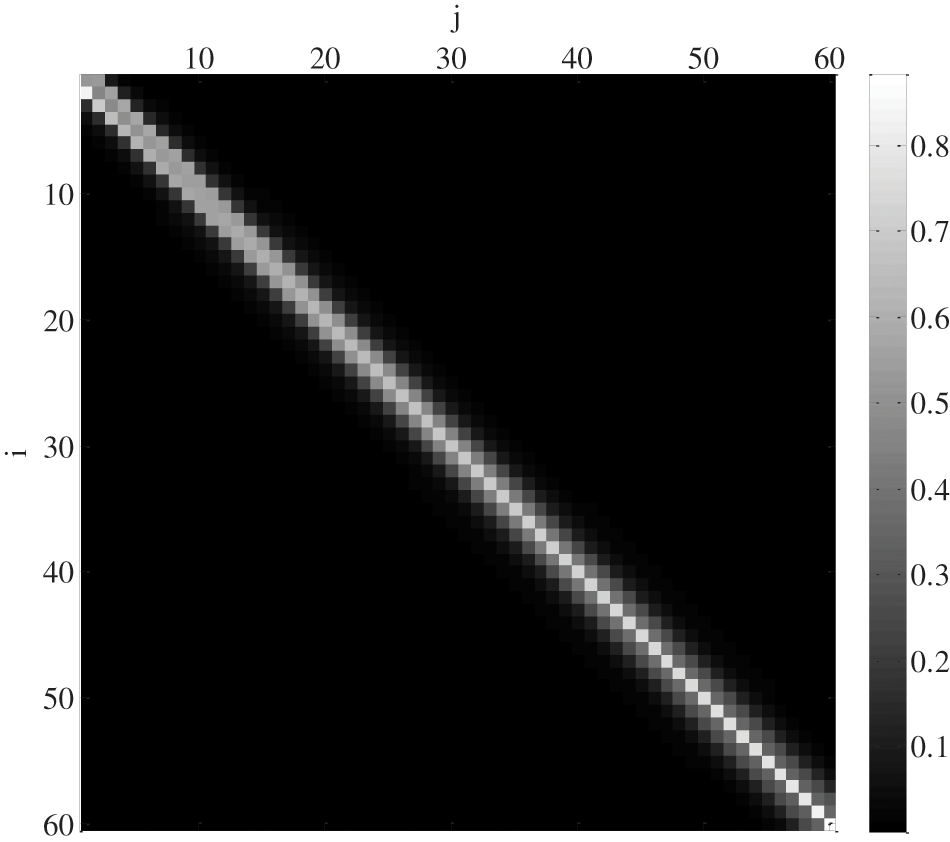
Figure 10: Absolute value of normalized system transfer matrix for the B sensors

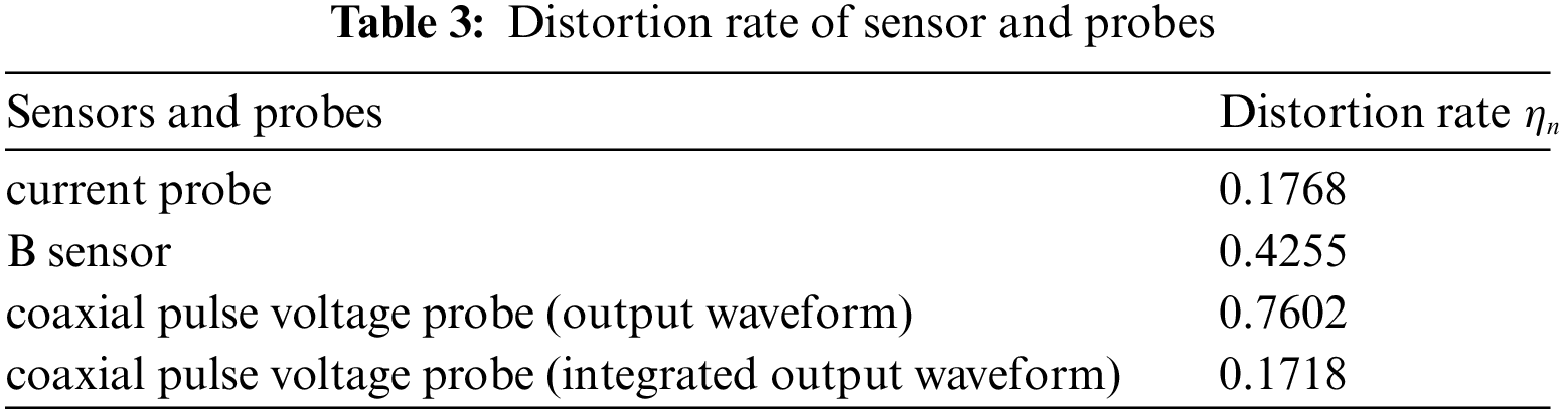
The distortion rates of the current probe, the coaxial pulse voltage probe and the B sensor are shown in Tab. 3. It can be seen from the table that the current probe has the smallest distortion rate; the differential output of the coaxial pulse voltage probe has the largest distortion rate; the B sensor is in between. It is because that the output of the current probe is proportional to the input, and the distortion is the minimum; the output of the coaxial pulse voltage probe is the differential of the input, and the distortion is the largest; the B sensor has both proportional output and differential output, and the distortion is between the current probe and the coaxial pulse voltage probe. For the coaxial pulse voltage probe, the distortion rate calculated from its direct output waveform is 0.7602, and the distortion rate calculated by integrating the waveform is reduced to 0.1718, which verifies the characteristics of differential sensor. The results of the above distortion rate analysis are consistent with those of the system transfer matrix analysis.

5  Conclusion

It is challenging for an EMP sensor to measure a wideband electromagnetic pulse without distortion for the whole spectrum. Therefore, analyzing the distortion of EMP measurement is crucial to evaluating the sensor distortion characteristics and correcting the measurement results. Waveform fidelity is usually employed to evaluate the distortion of an antenna. However, this metric depends on specific signal waveforms, thus is unsuitable for evaluating and analyzing the distortion of EMP sensors. In view of the limitation of the fidelity, an AH-function based distortion analysis method including system transfer matrices and distortion rates is proposed in this paper, which is general and independent from individual waveforms. The system transfer matrix and distortion rate can be straightforwardly calculated by the signal orthogonal decomposition coefficients using AH functions. According to a set of measured time-domain signal waveforms, the system transfer function is obtained by the orthogonal decomposition with AH basis function. Then, by exciting the transfer function using each order AH basis vector, there will be different outputs and the system transfer matrix can be established from orthogonal decomposition coefficients of those outputs. The distortion rate can be calculated by comparing the system transfer matrix with the identity matrix. Distortion of a sensor vs. frequency is then visualized via the system transfer matrix, which is convenient in quantitative analysis of the distortion. Finally, measurement of a current probe, a coaxial pulse voltage probe and a B-field sensor were performed, based on which the feasibility and effectiveness of the proposed distortion analysis method is successfully verified.

Funding Statement: Research Project of High-Level Talents of Jiangsu Police Institute (No.2911118010).

Conflicts of Interest: The authors declare that they have no conflicts of interest to report regarding the present study.

References

 1.  D. Zhou, M. X. Wei, L. H. Shi, J. Cao and L. Y. Su, “Experimental analysis of electromagnetic pulse effects on engine fuel electronic control system,” International Journal of Applied Electromagnetics and Mechanics, vol. 65, no. 1, pp. 45–57, 2021. [Google Scholar]

 2.  N. Dong, Y. L. Sun, Z. Y. Wang, Y. Z. Xie and Y. H. Chen, “Threat assessment method based on quantification of margins and uncertainties for electrical electronic equipment under high-altitude electromagnetic pulse,” High Power Laser and Particle Beams, vol. 33, no. 12, pp. 80–85, 2021. [Google Scholar]

 3.  Y. Zhou, Y. Z. Xie, D. Z. Zhang and Y. Jing, “Modeling and performance evaluation of inductive couplers for pulsed current injection,” IEEE Transactions on Electromagnetic Compatibility, vol. 63, no. 3, pp. 710–719, 2021. [Google Scholar]

 4.  Z. W. Gao, S. Zhang, L. Hao and N. Cao, “Modeling and analysis the effects of EMP on the balise system,” Computers, Materials & Continua, vol. 58, no. 3, pp. 859–878, 2019. [Google Scholar]

 5.  X. R. Zhang, W. Z. Zhang, W. Sun, H. L. Wu, A. G. Song et al., “A real-time cutting model based on finite element and order reduction,” Computer Systems Science and Engineering, vol. 43, no. 1, pp. 1–15, 2022. [Google Scholar]

 6.  F. Qin, Y. Gao and H. G. Ma, “Progress and prospect of high-confidence measurement technology for high-intensity electromagnetic pulse,” High Power Laser and Particle Beams, vol. 33, no. 12, pp. 1–12, 2021. [Google Scholar]

 7.  X. F. Yan, C. Q. Zhu and J. Wang, “Research and development of transient pulsed electric field sensor,” Nuclear Electronics & Detection Technology, vol. 39, no. 3, pp. 356–362, 2019. [Google Scholar]

 8.  P. Yang, G. Liu, X. Li, L. Qin and X. Liu, “An intelligent tumors coding method based on drools,” Journal of New Media, vol. 2, no. 3, pp. 111–119, 2020. [Google Scholar]

 9.  Y. J. Zhu, X. D. Guo and J. L. Song, “Design and sensitivity correction method of pulsed magnetic field sensor,” China Measurement & Testing Technology, vol. 45, no. 3, pp. 114–120, 2019. [Google Scholar]

10. W. Sun, Y. Y. Wang, X. L. Yao, Q. He and S. J. Hao, “Development of rogowski coil for 10/1000μs lightning current measurement,” Insulators and Surge Arresters, vol. 63, no. 5, pp. 1–6, 14, 2020. [Google Scholar]

11. N. A. Jan, S. H. Kiani, D. A. Sehrai, M. R. Anjum, A. Iqbal et al., “Design of a compact monopole antenna for uwb applications,” Computers, Materials & Continua, vol. 66, no. 1, pp. 35–44, 2021. [Google Scholar]

12. S. G. Mao and S. L. Chen, “Time-domain characteristic of ultra-wideband tapered loop antennas,” Electronics Letters, vol. 42, no. 22, pp. 1262–1263, 2006. [Google Scholar]

13. J. Yu and Z. X. Hao, “Design of a Novel UWB Antenna,” Radio Engineering, vol. 52, no. 5, pp. 859–863, 2022. [Google Scholar]

14. I. Mahariq, M. Kuzuoğlu, I. H. Tarman and H. Kurt, “Photonic nanojet analysis by spectral element method,” IEEE Photonics Journal, vol. 6, no. 5, pp. 1–14, 2014. [Google Scholar]

15. I. Mahariq, H. Kurt and M. Kuzuoğlu, “Questioning degree of accuracy offered by the spectral element method in computational electromagnetics,” Applied Computational Electromagnetics Society Journal (ACES), vol. 30, no. 7, pp. 698–705, 2015. [Google Scholar]

16. P. L. Carro and J. D. Mingo, “Ultrawide-band antenna distortion characterization using Hermite-Gauss signal subspaces,” IEEE Transactions on Antennas and Wireless Propagation Letters, vol. 7, pp. 267–270, 2008. [Google Scholar]

17. S. Saboktakin and B. Kordi, “Time-domain distortion analysis of wideband electromagnetic-field sensors using Hermite-Gauss orthogonal functions,” IEEE Transactions on Electromagnetic Compatibility, vol. 54, no. 3, pp. 511–521, 2012. [Google Scholar]

18. Z. Y. Huang, L. H. Shi and B. Chen, “The 3-D unconditionally stable associated hermite finite-difference time-domain method,” IEEE Transactions on Antennas and Propagation, vol. 68, no. 7, pp. 5534–5543, 2020. [Google Scholar]

19. M. T. Yuan, A. De, T. K. Sarkar, J. Koh and B. H. Jung, “Conditions for generation of stable and accurate hybrid TD-FD MoM solutions,” IEEE Transactions on Microwave Theory and Techniques, vol. 54, no. 6, pp. 2552–2563, 2006. [Google Scholar]

20. R. P. Ma, L. H. Shi, Z. Y. Huang and Y. H. Zhou, “EMP signal reconstruction using associated-hermite orthogonal functions,” IEEE Transactions on Electromagnetic Compatibility, vol. 56, no. 5, pp. 1242–1245, 2014. [Google Scholar]