Modified Differential Evolution Algorithm for Solving Dynamic Optimization with Existence of Infeasible Environments

1  Introduction

Dynamic constrained optimization is necessary for solving many real-world problems in various fields [1,2]. In it, it is assumed that the objective function and/or constraint functions change over time. In particular changes can occur in one or more of the coefficients of the objective function, coefficients of the constraint functions, right-hand side of the constraints, and variable bounds. In some cases, the function’s structure may be changed, and the addition and removal of constraints may occur. Here, we assume that each environment is represented by a problem instance. With the new environment, the problem instance may have a completely different or partially overlapped feasible space with an optimal solution probably located in a different place in the new feasible space. In such problems, the dynamics of the constraints impose more challenges that modify the shape and size of the feasible area [3]. In such a case, the objective of a solver is to find the best feasible solution in the current and subsequent environments. Examples of real-world dynamic problems include hydro-thermal scheduling [4] and ship scheduling [5].

Detecting changes in environments and tracking the changing optimum are two important tasks for solving dynamic optimization problems (DOPs). Many studies have been conducted to track the changing optimum [6–12]. Despite the large body of literature on solving dynamic problems, the majority of approaches focus mainly on unconstrained problems, while most real-world dynamic problems are dynamic constrained optimization problems (DCOPs) that have not yet been sufficiently explored. In DCOPs, handling constraints is an additional task dealt with using different methods [12,13]. However, solving DCOPs is computationally expensive [14,15] and their performances deteriorate if there are different types of changes in the environment [13–16].

To judge the performances of new algorithms, some synthetic constrained test problems, in which all instances are feasible, are proposed in the literature. However, in practice, some problem environments may not be feasible owing to various real-life issues; for example, their resource requirements can be significantly higher than expected due to defects in their supplied materials, shortages of resources in a given time period due to delivery disruptions, capacity reductions due to machine breakdowns and unexpected increases in market demand [17]. That means, it is possible that in some DCOPs, one or more problem instances can be infeasible, which does not suit decision-makers as infeasible solutions cannot be implemented. However, this does not mean that no activities will be performed in that time period. In this case, finding the closest feasible solution with suggestions for minimum changes in the problem instance would be beneficial for decision-makers. For example, it could be a suggestion to scale down activities for later continuation.

When solving optimization problems using EAs, it is necessary to define the search space, which is usually limited by variable bounds. The feasible space of a constrained problem is limited by both its constraint functions and variable bounds. For this reason, the feasible space is usually smaller than the search space, but they can be equal in some cases. To optimize a problem, we are interested in finding the best feasible solution, which is usually located on the boundary of the feasible space for most practical problems [18], but for some the optimum solution can be located inside this feasible space. If we can find the constraint limits that ensure feasibility, let us call this ‘limits of feasibility’, it is possible to suggest the nearest feasible solution for an infeasible problem instance.

Motivated by the above-mentioned facts, the aim of this paper is firstly, to develop a mechanism that determines the limits of feasibility, that can help to deal with possible infeasibility in problem instances. Secondly, a knowledge-transfer mechanism that will allow the retrieval and exploitation of solutions from past environments is proposed. Finally, to solve DCOPs with the existence of infeasible environments, a multi-operator-based differential evolution (DE) algorithm is developed by incorporating those two mechanisms. The performance of the proposed algorithm was tested by solving 13 single objective DCOPs with dynamic inequality constraints and compared its solutions with those of state-of-the-art dynamic constrained optimization algorithms. The experimental results revealed that the proposed approach can obtain high-quality solutions in a limited amount of time and is capable of dealing with infeasible instances, so it is suited for all environments.

The rest of this paper is organized as follows: in Section 2, EAs for solving DCOPs are reviewed; in Section 3, DCOPs are introduced and the proposed approach is explained in detail; in Section 4, the experimental results are discussed and the performance of the proposed method analyzed; and, finally, conclusions are drawn and future research directions suggested in Section 5.

2  Related Literature

As of the literature, evolutionary algorithms (EAs) are widely accepted as effective methods for solving static optimization problems. It is a common trend to extend EAs developed for static problems to solve dynamic ones. However, in this situation, they converge to an optimum by reducing the population’s diversity, which requires additional mechanisms to adapt to the changed environment if the final population of a previous environment is used as an initial population of the current environment [19]. It is to be noted that many approaches begin with the final population from the previous environment when a change is detected. However, this method does not help to transfer an effective learning experience from one environment to the next. There are several approaches for tracking the changing optimum, that include introducing diversity [4–6], diversity-maintaining [7,8], memory-based [9], prediction-based [10,11] and multi-population approaches [12–20].

Compared to DOPs, not much work has been proposed in the literature for solving DCOPs. Thus, some EAs originally designed for static problems were adapted to solve dynamic constrained ones. Singh et al. [21] adjusted an infeasibility-driven EA (IDEA) to handle changes using a shift-detecting technique. This strategy’s fundamental idea is that a random individual is chosen and tested in each generation as a change detector and when a change is observed, the entire population is re-assessed. The experimental results show the superior performance of this strategy to those of state-of-the-art algorithms for two test problems, although its detection capability may be affected if the detector is randomly selected.

A memory-based method is another EA strategy proposed for solving DCOPs. A study presented by Richter [16] focused on adapting an abstract memory strategy [22], with two memory schemes called censoring and blending suggested. In them, good individuals and their related data are stored for later use in constrained and unconstrained problems. From evaluating this proposed algorithm, the results reveal that using these two schemes while adjusting the strategy achieves better performance when compared to a penalty function. Its main drawback is that it works well on specific types of constrained dynamic problems, particularly cyclic ones.

In a study by Richter et al. [23], attention is paid to comparing the blending and censoring memory schemes with three other different strategies for a particular type of DCOP. The main idea in these problems is that both the objective function and constraints could vary in an asynchronous change pattern. From the experimental results obtained, it is observed that the memory-based schemes perform better than the random approaches. Generally, the former often suffer from solving problems with environmental changes that do not appear previously.

Ameca-Alducin et al. [24] proposed a diversity introduction mechanism by incorporating two popular DE variants and memory of the best-found solutions in the search. It detects changes in the objective function and/or constraints to elevate diversity in the population while following a new peak. Also, random immigrants and a local search operator are integrated to enable faster convergence. Nevertheless, it cannot support adequate diversity as an infeasible solution is always considered to be worse than a feasible one.

Also, some studies consider a repairing strategy for solving DCOPS. That by Pal et al. [25] attempts to improve solutions by proposing a GSA + Repair method within a gravitational search algorithm (GSA) [26]. Its key idea is that there is an infeasible solution that moves towards the nearest feasible one chosen from the best solutions available in the reference set. This method is evaluated, with the empirical results showing that it exhibits superior performances to those of other state-of-the-art algorithms. Two issues with this strategy are firstly, if the feasible space is small and, secondly, previously feasible individuals need to be re-checked to determine if they are still available when there is a change.

In another significant study proposed by Nguyen [27], DCOPs are solved using a set of algorithms and strategies. The algorithms consist of current dynamic optimization (DO) mechanisms (i.e., random-immigrant and hyper-mutation) and two constraint handling (CH) strategies which are repairing and stochastic ranking. However, there are some drawbacks of using DO and CH to solve DCOPs, which include tracking feasible moving regions, maintaining diversity, detecting changes, updating the feasibility and infeasibility balance, and searching outside the range.

Bu et al. [12] proposed the LTFR-DSPSO method to find and follow multiple disconnected feasible regions simultaneously using multiple sub-populations, each of which applies a gradient-based repair operator and local search to accelerate locating feasible areas and enhance exploiting them, respectively. Also, it employs a memory-based approach to track earlier found feasible areas by archiving previously found local optima and best solutions. Moreover, it involves a linear prediction method to predict the locations of future feasible areas.

Another strategy, called sensitive constraint detection, was introduced by Hamza et al. [13]. It attempts to offer meaningful information to help determine the movement of a solution in changing environments. One of its merits is that merging it with a search process accelerates the algorithm’s convergence. Also, using it with a multi-operator EA can be helpful for constrained dynamic problems. However its performance deteriorates when solving problems with relatively large changes.

3  Materials and Methods

In this section, a framework for solving DCOPs is proposed. Firstly, a brief review of the optimization algorithm employed in this paper is provided. Then, an overview of the proposed framework is presented and then details of its components are discussed.

3.1 MODE Optimizer

The optimizer used in this method is based on multi-operator differential evolution (MODE) [28], where a population of size NP is randomly generated within the search space. Then, the solutions are randomly divided into two equal sub-populations, each of which is randomly assigned to one of two distinct mutation strategies, namely, DE/current-to-p best or DE/rand-to-p best, to generate new offspring. A selection mechanism is conducted between every offspring and its parent to decide the fittest solutions that survive to the following generation. Then, based on improvements calculated using the three criteria of the feasibility rate, population diversity and quality of solutions, the sizes of the sub-populations are updated in the next generation.

3.2 Proposed Approach

3.2.1 Dynamic Constrained Optimization

A DCOP is an optimization problem in which one or more of the functions and/or parameters change over time. The functions include the objective function and constraint functions (i.e., constraint left-hand side). In a given environment, it is considered a static problem instance which does not change for a given time period (i.e., the duration of the environment). In general, a DCOP can be expressed as

min/maxf(x,t)(1)

subject to gk(x,t)≤0,∀k=1,2,…,K

he(x,t)=0,∀e=1,2,…,E

Lj(t)≤xt,j≤Uj(t),∀j=1,2,…,D

where x ∈ S(t) ⊂ RD(t), x = [xt,1, …, xt,j, …, xt,D(t)]T is a solution vector of D variables that varies over time t, and f a single objective function. This problem has K inequality constraints (gk(x)) and E equality ones (he(x)), and each decision variable (xt,j) has lower and upper bounds (Lj(t) and Uj(t), respectively). The feasible space (F (t)) ⊆ search space (S(t)), where a feasible solution for a time t is a point that fulfils all the constraints. The aim is to find a feasible solution in each environment which minimizes or maximizes f(x, t), with all feasible points described as: a feasible solution for a time t that meets all the constraints and satisfies the boundary limits.

DCOPs can be classified as one of three types based on the dynamics of its objective function and constraints as: 1) the objective function is dynamic and the constraints static [29]; 2) the objective function is static while the constraints are dynamic [13]; and 3) both the objective function and constraints are dynamic [30]. For all these categories, global solutions’ movement and appearance after each change is affected by the infeasible regions.

The structure of the proposed framework is shown in Algorithm 1. It starts by randomly generating an initial population (P) of size NP (i.e.,P={X1→,X2→,…,XNP→}), with each individual evaluated and the number of fitness evaluations (FEs) updated. Then, the limits of feasibility are determined using the limit of feasibility (LOF) algorithm introduced in Section 3.2.2.

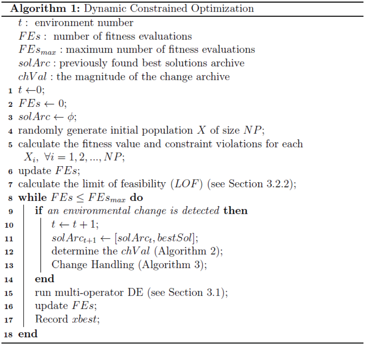
Next, the algorithm enters a loop (Algorithm 1, lines 8–18) which has two main phases: 1) a search and 2) a change-handling technique. In the first, the multi-operator DE algorithm [28] discussed in Section 3.1 is used to optimize the solution vector (X) until a change occurs. Then, the best solution is recorded before proceeding to the next phase which deals with the environmental changes and updates the population for the new environment. Although the proposed framework can adapt to any optimizer, in this paper, we selected MODE due to its good performance in solving optimization problems [13–31].

As many real-world DCOPs have cyclical changes [12,26], a previously found feasible solution may become a solution again after some time, and so tracking solutions in previous environments might be efficient. In this paper, a new strategy which tracks both the location information of the previous best feasible solutions and the change value, to handle environmental changes, is proposed. In it, previous solutions are retrieved based on the similarity in their change values with the current environment. Two archives are used, i.e., solArc(t) for the previously found best solutions in environment t and chngArc(t) for the magnitude of the environmental change.

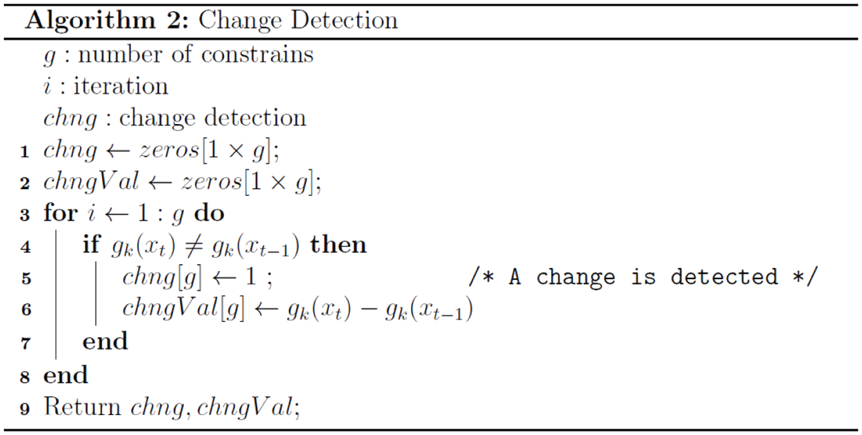
It is essential to identify when an environmental change occurs and its amount in many real-world DOPs [32]. A detector (i.e., certain individual) is employed to evaluate each constraint in the procedure for detecting change. A change occurs if the value of the detector in one environment is different from that in the previous one. Consequently, the change value is calculated as the difference between the evaluations in both environments, as described in Algorithm 2.

In changing environments, the constraints may alter in a way that a solution in the search space that was feasible in the previous environment may become infeasible. This may happen due to changes in the right-hand side values of the constraints (e.g., the availability of certain resources) and also changes in either the constraint coefficients or right-hand side values, or both. We assume that the variable bounds will be unchanged (although they can be changed), but the constraint right-hand-side values can be changed. No feasible solution means that no action can be taken and there is discontinuity in the actions between the environments, which is not acceptable in practice. To maintain continuity in actions, we believe it will be beneficial to find the nearest feasible solution so that the practitioner can make adjustments to the resources required. In other words, this will generate a feasible solution with minimum changes in the values on the right-hand side (Algorithm 3, lines 2–4). Since the new environment may be near the previous one, some solutions from the latter may be adopted. Therefore, to transfer the knowledge of promising solutions from the previous environment to the new one, k number of best solutions in the former will replace the worst individuals in the latter (Algorithm 3, lines 7–8). This number negatively correlates with the level of change, that is, k is small when chngVal is large and vice versa.

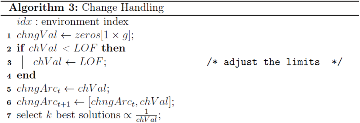
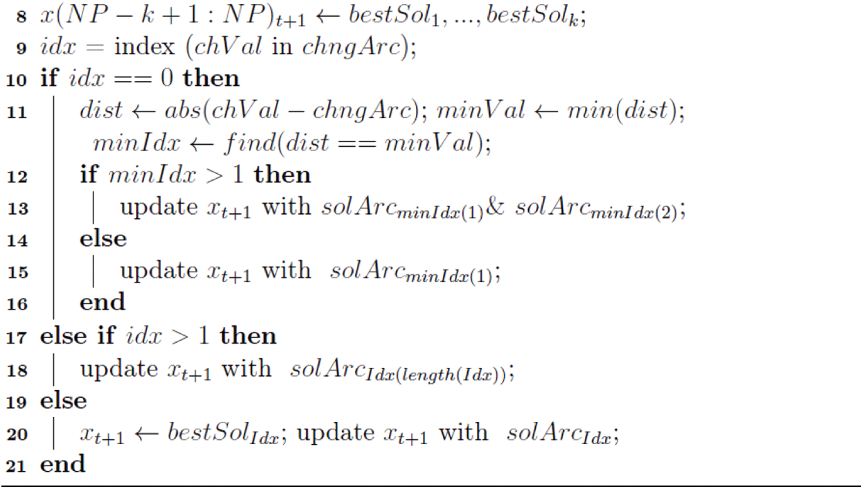
Also, as environments with the same change may have similar optimal solutions, solutions from previous environments are beneficial for use in a similar environment. The search process can start where other environments end (Algorithm 3, lines 9–21), which assists obtaining high-quality solutions in a limited amount of time. Firstly, the magnitude of change (chngVal) is used to measure the similarities between the current and all previous environments. Then, if a previous environment has the same chngVal as the current one, its best solution will be retained in the new one.

Another scenario may be where several previous environments have the same chngVal. In this situation, the algorithm selects solutions from the most recent one which includes higher-quality solutions. In contrast, if chngVal does not exist in chngArc, this environment did not previously appear. Therefore, the algorithm retains the best solutions from the nearest environment (i.e., has a chngVal closest to the current one) in the next environment. If there is more than one close environment, their best solutions will remain in the next one.

3.2.2 Feasibility Measures

In this section, in a case of infeasibility, the idea of finding the nearest feasible solution is discussed. Firstly, an analytical example is provided and then a genetic algorithm-based approach presented.

a)   Analytical Example

Let us consider a problem (G24 from [33]) as an example instance for a given environment, as

minf(x)=−x1−x2(2)

subject to g1(x)=−2x14+8x13−8x12+x2−2≤0

g2(x)=−4x14+32x13−88x12+96x1+x2−36≤0

where0≤x1≤3and0≤x2≤4

As previously discussed, to solve a problem using EAs, the search space considered is usually larger than the feasible space of the problem and is defined by the variable bounds, as shown in the mathematical model and Fig. 1. For different corner points of the search space, the constraints’ slacks and violations are presented in Tab. 1. In this problem, out of four corner points ((0, 0), (3, 0), (0, 4) and (3, 4)), two of them ((0, 4) and (3, 4)) are infeasible, which means that they are outside the feasible space, which is acceptable for our definitions of feasible and search spaces. However, at (0, 4), the violation is 2 units for g1(x) and, at (3, 4), 4 units for g2(x). The other two points are feasible as they are inside the constraints’ boundary. However, point (0, 0) has only 2 units slack for g1(x) and point (3, 0) is on the boundary of g2(x). The maximum slack is 20 for g1(x) at (3, 0) and 36 for g2(x) at (0, 0).

Figure 1: An analytical example of the G24 function that shows the slacks and violations of the corner points of the search space determined by the two inequality constraints g1(x) and g2(x)

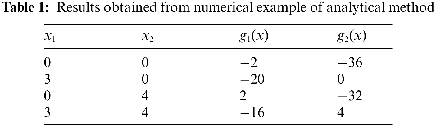
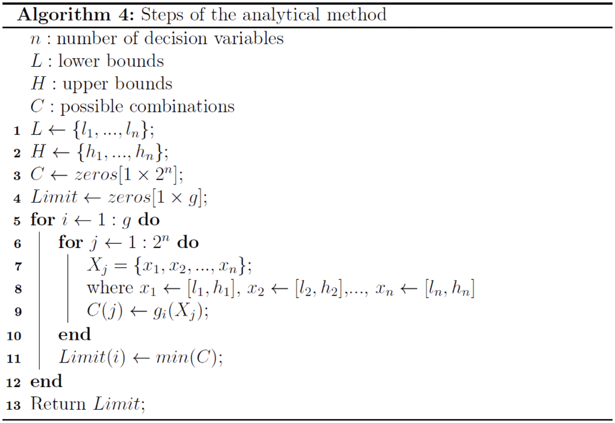
We assume that the search space is fixed but the feasible one may change due to a change in either the constraint function or right-hand side of the constraints or both. For any such variation, the optimal solution obtained in the previous environment may move to a new location in the new one and in some cases, can even be infeasible. In some situations, there may be no feasible solution if there is a large change in one or more constraints. In COPs, it is well known that the optimal solution often lies on the boundary of the feasible search space [18]. As the infeasible solution is not useful, we suggest a feasible one with minimum possible changes in the constraints. An analysis of the corner points of the search space, as discussed above, can be helpful for understanding the feasibility gaps between two consecutive environments. Therefore, in the analytical method shown in Algorithm 4, all the decision variables of a certain constraint (gk) are set to all possible combinations of its lower and upper bounds and then the corresponding constraint slacks or violations calculated. For less-than-equality constraints, the smallest value obtained is chosen to be the boundary limits of feasibility. This process is repeated until all the boundary limits are calculated. It is to be noted that the greater-than-equality and equality constraints can be converted to less-than-equality ones mathematically.

b)   Genetic-based Method

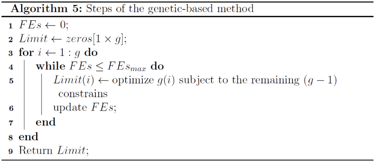
In the genetic-based method, to determine the limits of feasibility for each gk constraint, we use this constraint as an objective function that is evolved to determine its best slack value while satisfying all the remaining functional constraints and variable bounds. This value is then considered the boundary limits of feasibility for this gk constraint. This method is capable of handling cases in which the optimal solution lies either on the boundary of the feasible region or inside it. The same procedure is carried out until all the constraints are optimized. The pseudo-code of this method is presented in Algorithm 5.

4  Experimental Study

In this section, the performance of the proposed approach is analyzed by solving a set of benchmark functions introduced in the CEC2006 special competition sessions on COPs [33]. These test problems have different mathematical properties for the objective function and constraint(s). There are different types of objective functions, such as linear, nonlinear, polynomial, quadratic and cubic, while the constraints can be either equality or inequality ones. The proposed approach is tested on only the CEC2006 problems with inequality constraints. A dynamic version of these basic static functions is proposed by using time-dependent expressions for their parameters [13,34], including 13 benchmark problems with inequality constraints, namely, f1, f2, f4, f6-, f10, f12, f16, f18, f19 and f24.

For each benchmark problem, 25 independent runs were executed, each over 30 time periods with a change frequency of 5000 fitness evaluations (FEs). To find the limit of feasibility in the genetic approach, the optimizer is run 25 times for each constraint for up to FEsmax = 200,000. For MODE, the settings are the same as those reported in [28]. All the algorithms used in this manuscript were coded in MATLAB R2019b and experiments conducted on a PC with Intel Core i7 at 3.6 GHz and 16.0 GB of DDR3 main memory with a Windows 10 operating system.

4.1 Performance Measures

The average feasibility ratios and fitness values produced from all the experimental runs in each environment are used as performance measures. If feasible solutions were not obtained from the compared algorithms, the average sum of the constraint violations is considered the solutions’ quality measure. A statistical comparison is conducted using a Wilcoxon signed-rank test [35] with a 0.05 significance level. If the p-value is less than or equal to 5%, the null hypothesis is rejected; otherwise, it is accepted. The null hypothesis is there are no significant difference between the two algorithms. Whereas the alternative hypothesis is that there is a significant difference in the two algorithms’ values. The three signs +, - and ≈ designate that the first algorithm is either significantly better, worse than or not different from the second, respectively.

4.2 Experimental Results

In this section, the benefits of the proposed algorithm and its components are discussed and analyzed.

4.2.1 Finding Limits of Feasibility

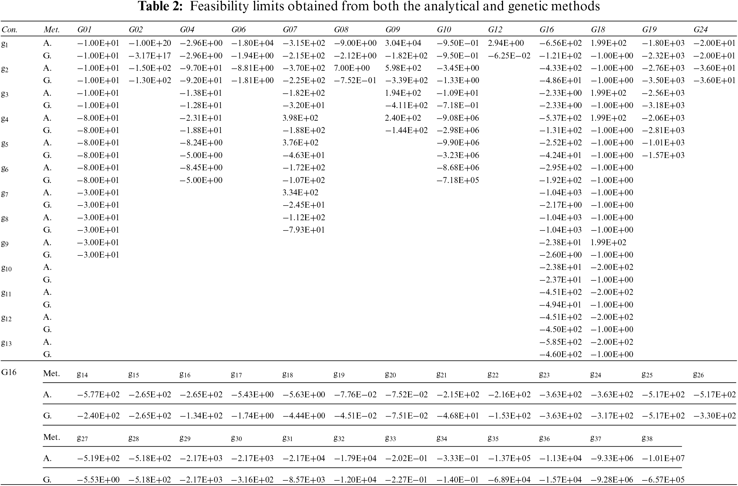
In this section, the results obtained from both the analytical and genetic methods are presented and discussed. Tab. 2 show the results obtained from both the analytical and genetic methods. It can be seen that the limits of feasibility are equal in both methods for some constraints, especially G01 and G24, as all the corresponding constraints have the same limit.

To evaluate the performances of the two different methods, these feasibility limits are applied on the dynamic variant of MODE [13] as a change in the right-hand side of each constraint. Therefore, this test environment contains the second type of combination of the objective function and constraints, with the former static and latter dynamic, and is formulated as

minf(x)(3)

subject to gk(x,t)≤boundaryk

where the change in constraints’ boundaries from 0 to boundaryk determines how the dynamic constraints change over time. Therefore, there are two time periods with their change frequencies set to 2.00E + 05 FEs.

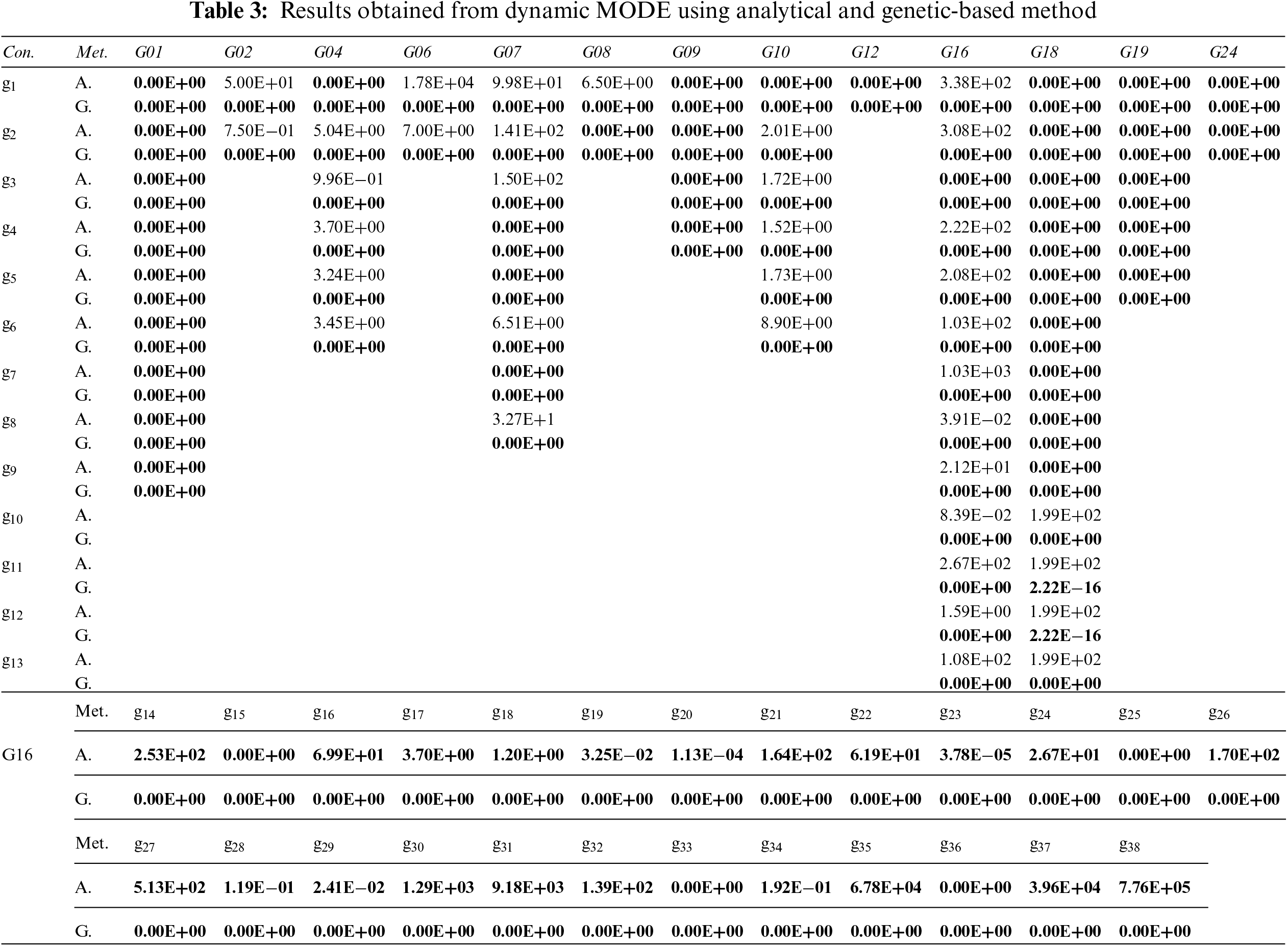
The experimental results obtained for each test problem from the analytical and genetic methods are illustrated in Tab. 3. Based on these results, it is obvious that the genetic and analytical approaches can find feasible solutions for 98 and 41 instances, respectively. Although many feasible solutions are obtained from the analytical method for several test problems, such as G09 and G19, their limits of feasibility may not be accurate, as those obtained from the genetic method are both smaller and feasible.

4.2.2 Benefits of Proposed Algorithm

In this subsection, the merits of the proposed framework are discussed based on comparisons of four different variants of the MODE algorithm. These include:

•   the proposed approach;

•   dynamic MODE using a sensitive constraint-detection mechanism [13];

•   default MODE initializing the population in each new environment with the population before a change occurs [28]; and

•   re-initialization MODE whereby the entire population is randomly re-initialized after every change [28].

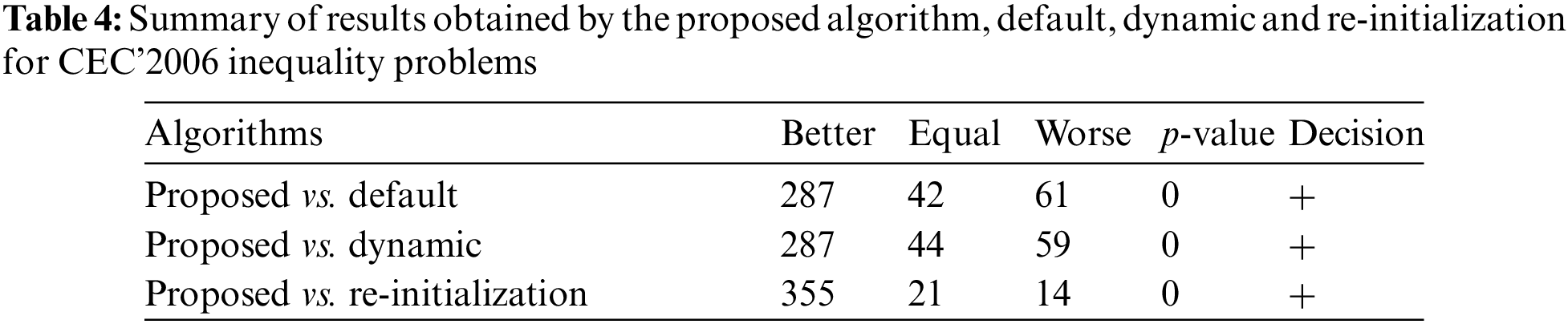
Detailed results are reported in the supplementary material in Appendices A and B, with summaries of the comparisons presented in Tab. 4. It can be observed that the performance of the proposed algorithm is superior to those of the other three variants as it obtains higher-quality solutions after the majority of environmental changes. Of the 1170 cases, it is superior, inferior and similar to the others for 929, 134 and 107, respectively. Therefore, it can be deduced that it performs better than the others for 79.40% of all the environments and is only outperformed for 11.45%.

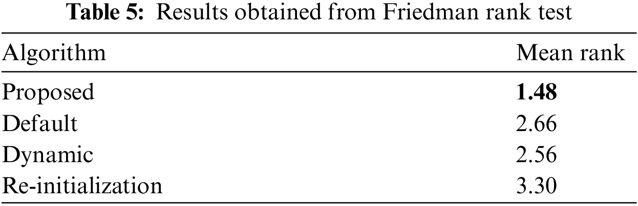
Furthermore, Tab. 5 shows the results obtained from the Friedman ranking test, that ranks all the variants according to the obtained mean results. From this table, it is demonstrated that the proposed algorithm ranks first (has the smallest value), as shown in bold, followed by MODE (dynamic), MODE (default) and MODE (re-initialization), respectively.

The proposed algorithm has superior performance because it tracks the useful location information of previous environments that helps to handle possible environmental changes. Also, it can deal with large changes effectively, which accelerates convergence towards feasibility and provides better solutions. However, the high violations of the constraints found in other variants lead to no feasible solutions. The experimental study shows the efficiency of the proposed method over the others, based on the results for most of the tested environments which, in turn, facilitates the movement of current solutions towards the feasible region.

Also, in order to better evaluate the proposed algorithm, the results obtained using the limits of feasibility for the other compared algorithms are shown in Tab. 6, with detailed results presented in supplementary documents in Appendices C and D. The results show the superiority of the proposed algorithm over MODE (default), MODE (dynamic) and MODE (re-initialization) in 259, 263 and 351 of 390 environments, respectively. This reveals the effectiveness of the proposed algorithm, even without using the limits of feasibility.

5  Conclusions

In this paper, a method for handling DCOPs under resource disruptions is introduced. In it, a mechanism that helps to locate useful information from previous environments when addressing DCOPs is developed. The solutions in previous environments are exploited in a new one based on their similarities. Also, when the constraints change so much that a solution lies in the infeasible area, the right-hand side of the original problem is modified to a limit that provides a feasible solution. Therefore, analytical and genetic methods for specifying the limits of feasibility, that can help address DCOPs under resource disruptions, are proposed.

The proposed algorithm is combined with an optimization one and used to test 13 DCOPs in each of which 30 dynamic changes occur with a frequency of 5000 FEs. The experimental results show that this proposed method outperforms other approaches and can handle big changes effectively, which accelerates convergence and achieves better solutions. The results also demonstrate that the genetic-based approach outperforms the analytical one for finding the limit of feasibility, as it is capable of providing more accurate results for such problems.

For possible future research, the proposed method could include a constraint-handling approach for bringing solutions back to the feasible region quickly when a disruption occurs. Also, as each mechanism has its advantages, a possible avenue of investigation is to choose the most suitable (i.e., either analytical or genetic) based on a problem’s characteristics. In addition, this implementation could be extended to consider dynamism in the objective function, variables’ boundaries and/or active variables.

Funding Statement: This research is supported by the Australian Research Council Discovery Project (Grant Nos. DP210102939).

Conflicts of Interest: The authors declare that they have no conflicts of interest to report regarding the present study.

References

1. Z. Zhang, S. Yue, M. Liao and F. Long, “Danger theory based artificial immune system solving dynamic constrained single-objective optimization,” Soft Computing, vol. 18, no. 1, pp. 185–206, 2014. [Google Scholar]
2. T. Zhu, W. Luo, C. Bu and L. Yue, “Accelerate population-based stochastic search algorithms with memory for optima tracking on dynamic power systems,” IEEE Transactions on Power Systems, vol. 31, no. 1, pp. 268–277, 2015. [Google Scholar]
3. T. T. Nguyen and X. Yao, “Continuous dynamic constrained optimization—The challenges,” IEEE Transactions on Evolutionary Computation, vol. 16, no. 6, pp. 769–786, 2012. [Google Scholar]
4. K. Deb, U. B. Rao N and S. Karthik, “Dynamic multi-objective optimization and decision-making using modified NSGA-II: A case study on hydro-thermal power scheduling,” in Proc. 4th Int. Conf. on Evolutionary Multi-Criterion Optimization (EMO), Matsushima, Japan, pp. 803–817, 2007. [Google Scholar]
5. K. Mertens, T. Holvoet and Y. Berbers, “The DynCOAA algorithm for dynamic constraint optimization problems,” in Proc. 5th Int. Joint Conf. on Autonomous Agents and Multiagent Systems (AAMAS), Hakodate, Japan, pp. 1421–1423, 2006. [Google Scholar]
6. D. Parrott and X. Li, “Locating and tracking multiple dynamic optima by a particle swarm model using speciation,” IEEE Transactions on Evolutionary Computation, vol. 10, no. 4, pp. 440–458, 2006. [Google Scholar]
7. T. Blackwell and J. Branke, “Multiswarms, exclusion, and anti-convergence in dynamic environments,” IEEE Transactions on Evolutionary Computation, vol. 10, no. 4, pp. 459–472, 2006. [Google Scholar]
8. S. Das, A. Mandal and R. Mukherjee, “An adaptive differential evolution algorithm for global optimization in dynamic environments,” IEEE Transactions on Cybernetics, vol. 44, no. 6, pp. 966–978, 2013. [Google Scholar]
9. W. Luo, J. Sun, C. Bu and H. Liang, “Species-based particle swarm optimizer enhanced by memory for dynamic optimization,” Applied Soft Computing, vol. 47, pp. 130–140, 2016. [Google Scholar]
10. A. Ahrari, S. Elsayed, R. Sarker, D. Essam and C. A. C. Coello, “Adaptive multilevel prediction method for dynamic multimodal optimization,” IEEE Transactions on Evolutionary Computation, vol. 25, no. 3, pp. 463–477, 2021. [Google Scholar]
11. M. Jiang, Z. Huang, L. Qiu, W. Huang and G. G. Yen, “Transfer learning-based dynamic multiobjective optimization algorithms,” IEEE Transactions on Evolutionary Computation, vol. 22, no. 4, pp. 501–514, 2017. [Google Scholar]
12. C. Bu, W. Luo and L. Yue, “Continuous dynamic constrained optimization with ensemble of locating and tracking feasible regions strategies,” IEEE Transactions on Evolutionary Computation, vol. 21, no. 1, pp. 14–33, 2017. [Google Scholar]
13. N. Hamza, R. Sarker and D. Essam, “Sensitivity-based change detection for dynamic constrained optimization,” IEEE Access, vol. 8, pp. 103900–103912, 2020. [Google Scholar]
14. M. -Y. Ameca-Alducin, E. Mezura-Montes and N. Cruz-Ramírez, “Differential evolution with a repair method to solve dynamic constrained optimization problems,” in Proc. of Genetic and Evolutionary Computation Conf. (GECCO), New York, NY, USA, pp. 1169–1172, 2015. [Google Scholar]
15. M. -Y. Ameca-Alducin, E. Mezura-Montes and N. Cruz-Ramírez, “A repair method for differential evolution with combined variants to solve dynamic constrained optimization problems,” in Proc. of Genetic and Evolutionary Computation Conf. (GECCO), New York, NY, USA, pp. 241–248, 2015. [Google Scholar]
16. H. Richter, “Memory design for constrained dynamic optimization problems,” in European Conf. on the Applications of Evolutionary Computation, Istanbul, Turkey, pp. 552–561, 2010. [Google Scholar]
17. F. Zaman, S. Elsayed, R. Sarker, D. Essam and C. A. C. Coello, “Pro-reactive approach for project scheduling under unpredictable disruptions,” IEEE Transactions on Cybernetics, pp. 1–14, 2021. https://doi.org.10.1109/TCYB.2021.3097312. [Google Scholar]
18. M. R. Bonyadi and Z. Michalewicz, “On the edge of feasibility: A case study of the particle swarm optimizer,” in Proc. IEEE Congress on Evolutionary Computation (CEC), Beijing, China, pp. 3059–3066, 2014. [Google Scholar]
19. J. Branke, “Evolutionary optimization in dynamic environments,” in Genetic Algorithms and Evolutionary Computation, vol. 3. New York, NY, USA: Springer, 2012. [Google Scholar]
20. D. Yazdani, M. N. Omidvar, J. Branke, T. T. Nguyen and X. Yao, “Scaling up dynamic optimization problems: A divide-and-conquer approach,” IEEE Transactions on Evolutionary Computation, vol. 24, no. 1, pp. 1–15, 2019. [Google Scholar]
21. H. K. Singh, A. Isaacs, T. T. Nguyen, T. Ray and X. Yao, “Performance of infeasibility driven evolutionary algorithm (IDEA) on constrained dynamic single objective optimization problems,” in Proc. IEEE Congress on Evolutionary Computation (CEC), Trondheim, Norway, pp. 3127–3134, 2009. [Google Scholar]
22. H. Richter and S. Yang, “Memory based on abstraction for dynamic fitness functions,” in Workshops on Applications of Evolutionary Computation, Naples, Italy, pp. 596–605, 2008. [Google Scholar]
23. H. Richter and F. Dietel, “Solving dynamic constrained optimization problems with asynchronous change pattern,” in Proc. European Conf. on the Applications of Evolutionary Computation, Torino, Italy, pp. 334–343, 2011. [Google Scholar]
24. M. -Y. Ameca-Alducin, E. Mezura-Montes and N. Cruz-Ramirez, “Differential evolution with combined variants for dynamic constrained optimization,” in Proc. IEEE Congress on Evolutionary Computation (CEC), Beijing, China, pp. 975–982, 2014. [Google Scholar]
25. K. Pal, C. Saha, S. Das and C. A. C. Coello, “Dynamic constrained optimization with offspring repair based gravitational search algorithm,” in Proc. IEEE Congress on Evolutionary Computation (CEC), Cancun, Mexico, pp. 2414–2421, 2013. [Google Scholar]
26. E. Rashedi, H. Nezamabadi-Pour and S. Saryazdi, “GSA: A gravitational search algorithm,” Information Sciences, vol. 179, no. 13, pp. 2232–2248, 2009. [Google Scholar]
27. T. T. Nguyen, “Continuous dynamic optimisation using evolutionary algorithms,” Ph.D. dissertation, University of Birmingham, England, 2011. [Google Scholar]
28. S. Elsayed, R. Sarker and C. C. Coello, “Enhanced multi-operator differential evolution for constrained optimization,” in Proc. IEEE Congress on Evolutionary Computation (CEC), Vancouver, BC, Canada, pp. 4191–4198, 2016. [Google Scholar]
29. L. Araujo and J. J. Merelo, “A genetic algorithm for dynamic modelling and prediction of activity in document streams,” in Proc. of Genetic and Evolutionary Computation Conf. (GECCO), London, United Kingdom, pp. 1896–1903, 2007. [Google Scholar]
30. Y. Wang and M. Wineberg, “Estimation of evolvability genetic algorithm and dynamic environments,” Genetic Programming and Evolvable Machines, vol. 7, no. 4, pp. 355–382, 2006. [Google Scholar]
31. S. Elsayed, R. Sarker, N. Hamza, C. A. C. Coello and E. Mezura-Montes, “Enhancing evolutionary algorithms by efficient population initialization for constrained problems,” in Proc. IEEE Congress on Evolutionary Computation (CEC), Glasgow, United Kingdom, pp. 1–8, 2020. [Google Scholar]
32. D. Yazdani, R. Cheng, D. Yazdani, J. Branke, Y. Jin et al., “A survey of evolutionary continuous dynamic optimization over two decades–part b,” IEEE Transactions on Evolutionary Computation, vol. 25, no. 4, pp. 609–629, 2021. [Google Scholar]
33. J. J. Liang, T. P. Runarsson, E. Mezura-Montes, M. Clerc, P. N. Suganthan et al., “Problem definitions and evaluation criteria for the CEC 2006 special session on constrained real-parameter optimization,” Journal of Applied Mechanics, vol. 41, no. 8, pp. 8–31, 2006. [Google Scholar]
34. T. T. Nguyen, “A proposed real-valued dynamic constrained benchmark set,” School of Computer Science, Univesity of Birmingham, Tech. Rep., pp. 1–54, 2008. [Google Scholar]
35. G. Corder and D. Foreman, “Nonparametric statistics: An introduction,” in Nonparametric Statistics for Non-Statisticians: A Step-by-Step Approach, Hoboken, NJ, USA: Wiley, pp. 101–111, 2009. [Google Scholar]
Cite This Article
Copyright © 2023 The Author(s). Published by Tech Science Press.
This work is licensed under a Creative Commons Attribution 4.0 International License , which permits unrestricted use, distribution, and reproduction in any medium, provided the original work is properly cited.
Downloads
Citation Tools