Computers, Materials & Continua DOI:10.32604/cmc.2022.030694
Article

Optimal Logistics Activities Based Deep Learning Enabled Traffic Flow Prediction Model

Basim Aljabhan1, Mahmoud Ragab2,3,4,*, Sultanah M. Alshammari4,5 and Abdullah S. Al-Malaise Al-Ghamdi4,6,7

1Ports and Maritime Transportation Department, Faculty of Maritime Studies, King Abdulaziz University, Jeddah, 21589,  Saudi Arabia
2Information Technology Department, Faculty of Computing and Information Technology, King Abdulaziz University, Jeddah, 21589, Saudi Arabia
3Department of Mathematics, Faculty of Science, Al-Azhar University, Naser City, 11884, Cairo, Egypt
4Center of Excellence in Smart Environment Research, King Abdulaziz University, Jeddah, 21589, Saudi Arabia
5Department of Computer Science, Faculty of Computing and Information Technology, King Abdulaziz University, Jeddah, 21589, Saudi Arabia
6Information Systems Department, Faculty of Computing and Information Technology, King Abdulaziz University, Jeddah, 21589, Saudi Arabia
7Information Systems Department, HECI School, Dar Alhekma University, Jeddah, Saudi Arabia
*Corresponding Author: Mahmoud Ragab. Email: mragab@kau.edu.sa
Received: 31 March 2022; Accepted: 19 May 2022

Abstract: Traffic flow prediction becomes an essential process for intelligent transportation systems (ITS). Though traffic sensor devices are manually controllable, traffic flow data with distinct length, uneven sampling, and missing data finds challenging for effective exploitation. The traffic data has been considerably increased in recent times which cannot be handled by traditional mathematical models. The recent developments of statistic and deep learning (DL) models pave a way for the effectual design of traffic flow prediction (TFP) models. In this view, this study designs optimal attention-based deep learning with statistical analysis for TFP (OADLSA-TFP) model. The presented OADLSA-TFP model intends to effectually forecast the level of traffic in the environment. To attain this, the OADLSA-TFP model employs attention-based bidirectional long short-term memory (ABLSTM) model for predicting traffic flow. In order to enhance the performance of the ABLSTM model, the hyperparameter optimization process is performed using artificial fish swarm algorithm (AFSA). A wide-ranging experimental analysis is carried out on benchmark dataset and the obtained values reported the enhancements of the OADLSA-TFP model over the recent approaches mean square error (MSE), root mean square error (RMSE), and mean absolute percentage error (MAPE) of 120.342%, 10.970%, and 8.146% respectively.

Keywords: Traffic flow prediction; deep learning; artificial fish swarm algorithm; mass gatherings; statistical analysis; logistics

1  Introduction

Currently, timely and accurate traffic flow data is powerfully required for government agencies, business sectors and individual travelers, and business sectors [1]. Traffic data helps road users to alleviate traffic congestion, take effective travel decisions, enhance traffic operation efficacy, and decrease carbon emission. The density of logistics activities and its value as a key economic activity has increased the structure of information and communication technology (ICT) as process to enhance the levels of responsiveness, efficiency and visibility in supply chains relying in multimodal transport operations. The aim of traffic flow prediction (TFP) is to offer traffic flow data. TFP is a significant module of traffic management, modelling, and operation [2]. Accurate real-time TFP offer guidance and information for road user to reduce cost and to improve travel decision. Also, it assists authorities with traffic management strategies to lessen congestion, predict crowd density, behavior contact and mobility patterns in mass gatherings events during emergency situations in smart environment.

With the accessibility of higher resolution traffic information from intelligent transportation systems (ITS), TFP was gradually tackled with data driven approach [3]. TFP is based largely on real-time traffic and historical information gathered from different sensors, including radars, inductive loops, mobile Global Positioning System (GPS), cameras, social media, crowd sourcing, and so on. With the conventional traffic sensor and emergent traffic sensor technology, traffic information is exploding and has entered the period of big data transport systems. Now, transport control and its management systems become additional data driven [4,5].

Even though there are previously numerous TFP models and schemes, many of them utilize shallow traffic systems and still are slightly unsatisfactory. This stimulates reconsideration the TFP issue depends on deep structure model with large quantity of traffic information [6]. In recent times, deep learning (DL) that is a kind of machine learning (ML) technique, has gained considerable interest in industrial and interest fields [7]. It is employed with achievement in reduction dimension, classification task, natural language processing (NLP), motion modeling, object detection, etc. [8]. The DL algorithm uses many deep architectures or layer architectures for extracting intrinsic characteristics in information from the minimum level to the maximum level and determining massive number of architecture in the information. Since a traffic flow progression is difficult naturally, DL algorithm represents traffic feature without previous knowledge that has better efficacy for TFP [9,10]. Fig. 1 depicts the role of artificial intelligence (AI) in Internet of Things (IoT).

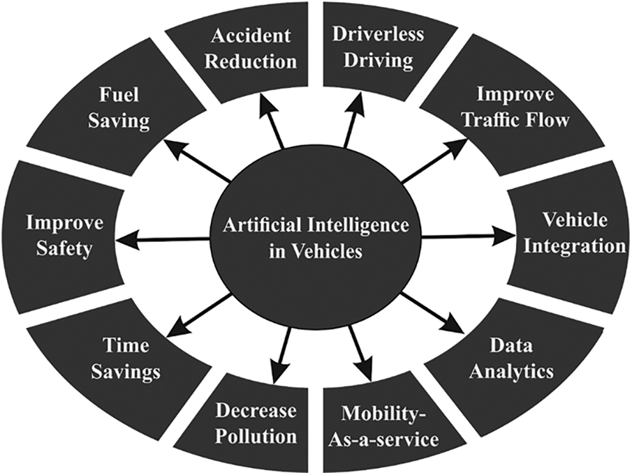
Figure 1: Role of artificial intelligence (AI) in the Internet of Things (IoT)

Yang et al. [11] presented an enhanced method which attaches the maximum control value of remarkably long structure time-steps to existing time-step, and these maximum control traffic flow values were captured utilizing the attention process. Simultaneously, it can be smooth out several data further than the normal range for obtaining optimum predictive outcomes. Liu et al. [12] presented a privacy-preserving ML approach called federated learning (FL) and present an FL based gated recurrent unit-neural network (GRU-NN) technique (FedGRU) for TFP. In FedGRU varies in existing centralized learning approaches and upgrades universal learning approaches with a secured parameter aggregation system before directly sharing raw data amongst organizations.

Chen et al. [13] established data denoising methods (such as Wavelet (WL), Empirical Mode Decomposition (EMD), and Ensemble EMD (EEMD)) for suppressing the potential data outlier. Next, the LSTM-NN has been established for fulfilling the TFP task. Tang et al. [14] widely estimated the multi-step predictive efficiency of models with distinct denoising techniques utilizing the traffic volume data gathered in 3 loop detector placed on highway in city of Minneapolis. During the predictive efficiency comparison, 5 denoising approaches were utilized. Tao et al. [15] presented a pragmatic system with executing the efficient hinging hyperplanes neural network (EHHNN) easily created on sparse neuron connection. During the presented approach, distinct traffic features were combined as to the inputs containing its spatial-temporal data. Also, the detection of accuracy can be more extended the statistical decomposition of EHHNNs to interpretation analysis with specification for traffic information whereas the contribution regarding particular traffic variable is noticed quantitatively.

This study designs optimal attention-based deep learning with statistical analysis for TFP (OADLSA-TFP) model. The presented OADLSA-TFP model intends to effectually forecast the level of traffic in the environment. To attain this, the OADLSA-TFP model employs attention-based bidirectional long short-term memory (ABLSTM) model for predicting traffic flow. In order to enhance the performance of the ABLSTM model, the hyperparameter optimization process is performed using artificial fish swarm algorithm (AFSA). A wide-ranging experimental analysis is carried out on benchmark dataset and the obtained values reported the enhancements of the OADLSA-TFP model over the recent approaches.

2  The Proposed Model

In this study, a novel OADLSA-TFP model has been developed to effectually forecast the level of traffic in the environment. The OADLSA-TFP model primarily employed the design of ABLSTM model for predicting traffic flow. In order to enhance the performance of the ABLSTM model, the hyperparameter optimization process is performed using AFSA and thereby boosts the predictive results.

2.1 Process Involved in ABLSTM Based Prediction

At the initial stage, the OADLSA-TFP model primarily employed the design of ABLSTM model for predicting traffic flow. Consider I={i1,i2,i3,………,it} represent the set of encoded identifiers of source code [16]. Then, An RNN implements for encoded ID it for t=1 to n. The output vector of recurrent neural network (RNN) yt is formulated by:

ht=tanh(Wxhxt+Whhht−1+bh)(1)

yt=Whyht+by(2)

whereas W denotes a weight matrix Wxh indicates a weight connecting input (x) to hidden stage (h), ht indicates the hidden output, tanh signifies an activation function, and b represents a bias vector of the hidden state. Eq. (1) is utilized for calculating the hidden output, whereas the hidden layer receives the result of the preceding layer.

But because of the gradient exploding or vanishing problem [17], each input sequence is effectively utilized in RNN. To produce a better result and prevent the problem, the RNN is expanded to long short term memory (LSTM). Theoretically, an LSTM network is analogous to RNN, however, the hidden state updating procedure can be replaced by a special unit named a memory cell. It can be expressed in the following:

it=σ(Wxixt+Whiht−1+Wcict−1+bi)(3)

ft=σ(Wxfxt+Whfht−1+Wcfct−1+bf)(4)

ct=ftct−1+ittan⁡h(Wxcxt+Whcht−1+bc)(5)

0t=σ(Wxoxt+Whoht−1+Wcoct+b0)(6)

ht=ottan⁡h(ct)(7)

In which σ denotes a sigmoid function; c,f,i, and o indicates the cell state, forget gate, input, and output; and b denotes bias function.

During this case, it can be integrated a bidirectional LSTM (BiLSTM) network with attention process. The BiLSTM network procedures input in two approaches: primary, it procedures data in the backward to forward directions, next it procedures the similar input in forward to backward. The BiLSTM technique varies in unidirectional LSTM as the network run the similar input twice, for instance, in forward to backward and backward to forward directions that preserve the further context data which is extremely useful from tourism demand predict for improving the network accuracy more. In the two input attention layers were utilized, one for feature and one for time step dimensional. The formula demonstrates the attention layer on input XT. Afterward input feature, attention process was executed before the BiLSTM layer. During the next step, the softmax function that offers the probability was executed and the next multiplication was utilized by the feature vector. The outcome in this layer is then sent to BiLSTM network, whereas the network learned the long-term dependency and is then sent to dense layer (left side from the figure) which offers the outcome.

AT=softmax(WT×[[Xt]t=1T]T+bT)×[[Xt]t=1T]T,(8)

AT=softmax(WT×[[Xt]t=1T]T+bT)×[[Xt]t=1T]T,(9)

whereas input XT has the T time step of F feature from a vector procedure. The softmax function takes a F×T dimensional vector that is a multiplication of time step T and n feature vectors F from the input vector. WT WF bT and bF are the parameter that is learned under the training. Fig. 2 demonstrates the framework of BiLSTM.

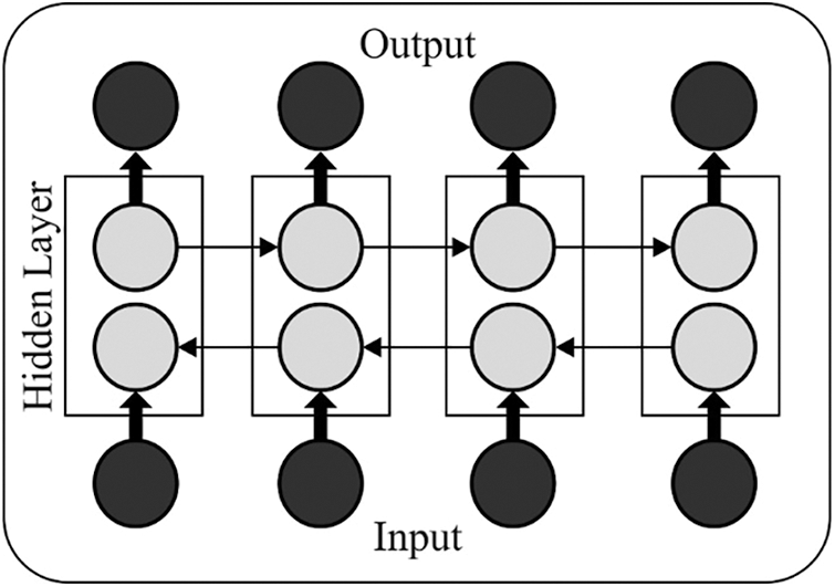
Figure 2: Structure of BiLSTM

2.2 Hyperparameter Optimization

Next, the hyperparameter optimization [18–20] process of the ABLSTM model is performed using AFSA and thereby boosts the predictive results. The AFSA is an existing swarm based optimized approach projected [21] and it could depend on flora migration and reproduction process. It can be found on 6 normal functions and illustrates the powerful exploration abilities with fast convergence. During this approach, an original plant was created initially and the scattered seeds are identified as off-spring plants, with a particular distance. Primarily, the early population was generated arbitrarily with N original plants.

Xi,j=r×D×2−D(10)

In which the original plant place was signified as Xi,j, i and j refer the dimension and amount of plants correspondingly, also r signifies the uniform distribution in the range of zero and one. Afterward, the propagating distance Dj was measured to every plant. The calculation of propagating distance of plants was dependent upon prior 2 generations.

Dj=D1j×r×c1+D2j×r×c2(11)

whereas propagation distances of grandparent and parent plants represent D2j and D1j correspondingly, c1 and c2 signifies the learning co-efficient, and r signifies the uniform distributing. The novel grandparent propagate is offered as:

D1j′=D2j(12)

A novel parent distribution distance was offered as:

D2j′=∑i=1N(Xij−Xij′)2N(13)

The off-spring plant places toward the original plant were evaluated as:

Xi,j×m′=Rij×m+Xi,j(14)

whereas Xij′ implies the off-spring plant places, m refers the count of off-spring was generated with single plant, and Ri,j×m refers the normal distributing arbitrary amount by mean zeroand variance Dj. Some generated off-spring is survived and others, also off-spring was alive/not is determined as the likelihood of survived that was evaluated employing proportion-based election.

p=|F(Xij×m′)Fmax|×Qj×˙m−1)(15)

In which the selected probability was signified as Q(j×m−1) and their value was amongst [0,1],Fmax signifies the maximal fitness of entire off-spring, and all the single off-spring plant represent F(Xi,j×m′). The off-spring is continued if the probability of surviving p was superior related to r, whereas r signifies the uniform distribution of arbitrary amounts from the interval [0,1]. The N off-spring plant was selected by continued off-spring as new original plant for subsequent iteration. The AFSA approach was frequent still it encounter the termination criteria. Eventually, a better outcome was chosen.

3  Experimental Validation

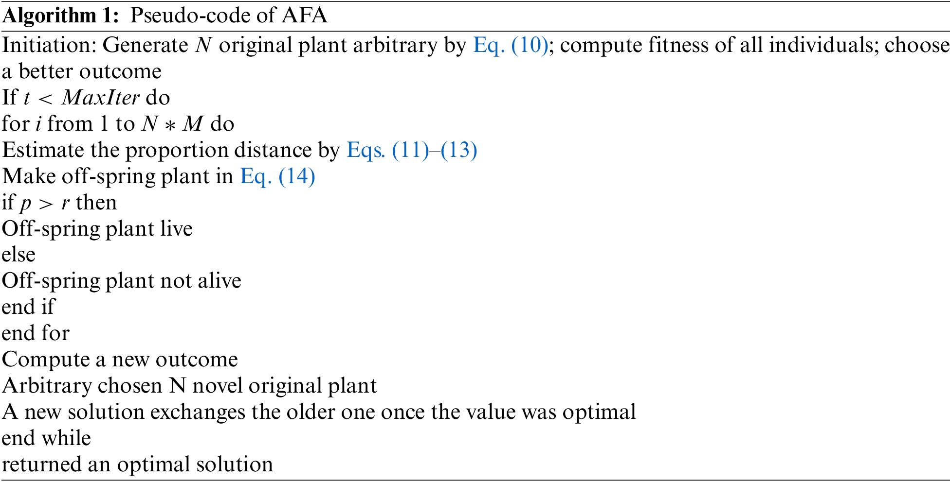
This section assesses the predictive performance of the OADLSA-TFP model under several aspects. Tab. 1 and Fig. 3 offer a detailed comparative study of the OADLSA-TFP model with existing models on weather data interms of mean square error (MSE), root mean square error (RMSE), and mean absolute percentage error (MAPE). The experimental results implied that the OADLSA-TFP model has accomplished effectual outcomes over the other techniques such as radial basis function (RBF) based prediction (RBF-P), RBF with Pearson Correlation Coefficient (RBF-PCC), RBF with Principal Component Analysis (RBF-PCA), hybrid RBF, and AI based TFP (AITFP).

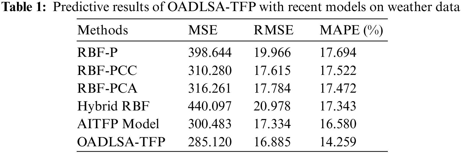
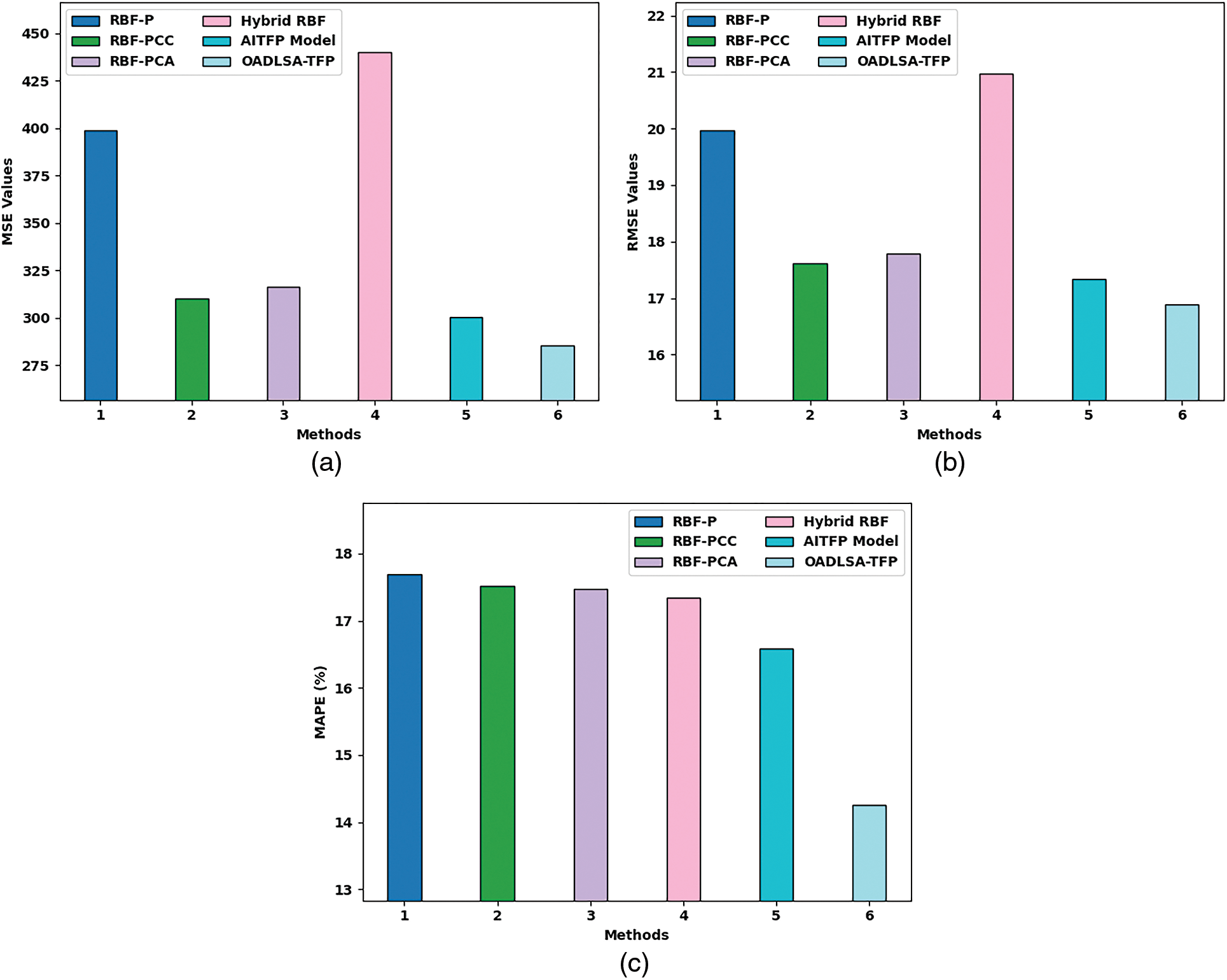
Figure 3: Overall predictive results of OADLSA-TFP with recent models on weather data (a) MSE, (b) RMSE, (c) MAPE

With respect to MSE, the OADLSA-TFP model has provided lower MSE of 285.120 whereas the RBF-P, RBF-PCC, RBF-PCA, Hybrid RBF, and AITFP models have offered higher MSE of 398.644, 310.280, 316.261, 440.097, and 300.483 respectively. Moreover, with respect to MAPE, the OADLSA-TFP model has gained least MAPE of 14.259% whereas the RBF-P, RBF-PCC, RBF-PCA, Hybrid RBF, and AITFP models have offered higher MAPE of 17.694%, 17.522%, 17.472%, 17.343%, and 16.580% respectively.

Next, a comprehensive comparative study of the OADLSA-TFP model with recent models is made in Tab. 2 and Fig. 4. The results indicated that the LSTM, GRU, and cascaded LSTM models have shown worse performance with increased error values. In addition, the Cascaded GRU, stacked encoder, F-ANN, and SAERBF models have gained slightly reduced error values. Though the AITFP-WC model has accomplished reasonable MSE, RMSE, and MAPE of 127.762%, 11.303%, and 9.724%, the presented OADLSA-TFP model has gained effectual outcome with MSE, RMSE, and MAPE of 120.342%, 10.970%, and 8.146% respectively.

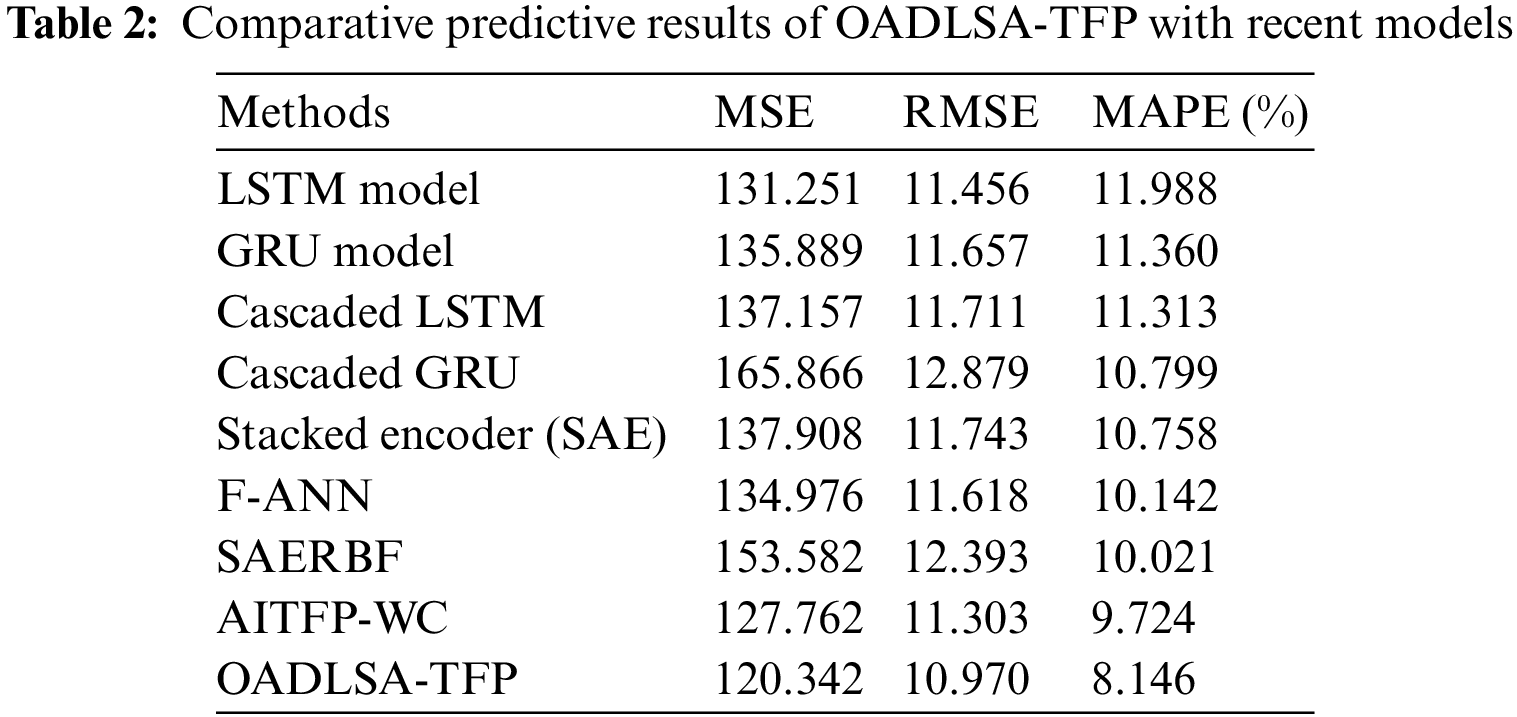
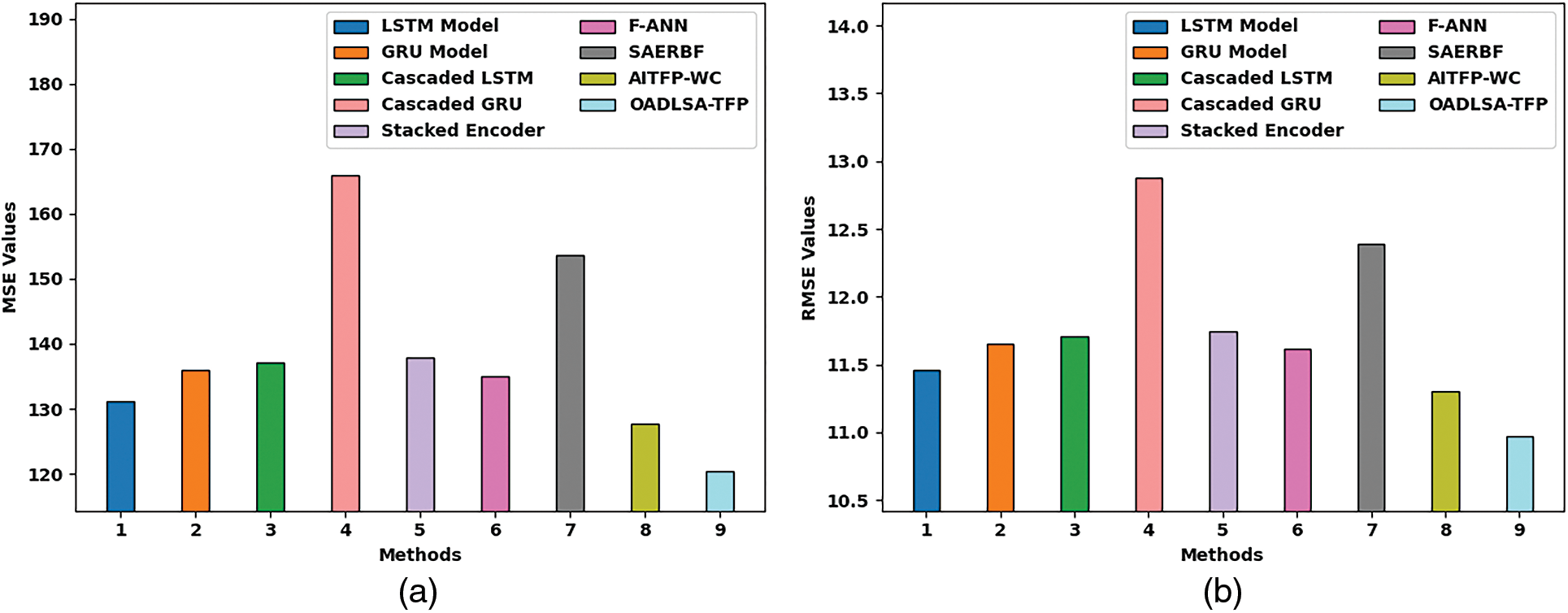
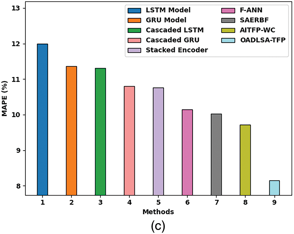
Figure 4: Comparative predictive results of OADLSA-TFP with recent models (a) MSE, (b) RMSE, (c) MAPE

Tab. 3 and Fig. 5 offer an MSE examination of the OADLSA-TFP model with existing ones under distinct durations. The results implied that the OADLSA-TFP model has shown improved performance with minimal values of MSE under all-time durations. For instance, with 5_min, the OADLSA-TFP model has offered reduced MSE of 120.342.

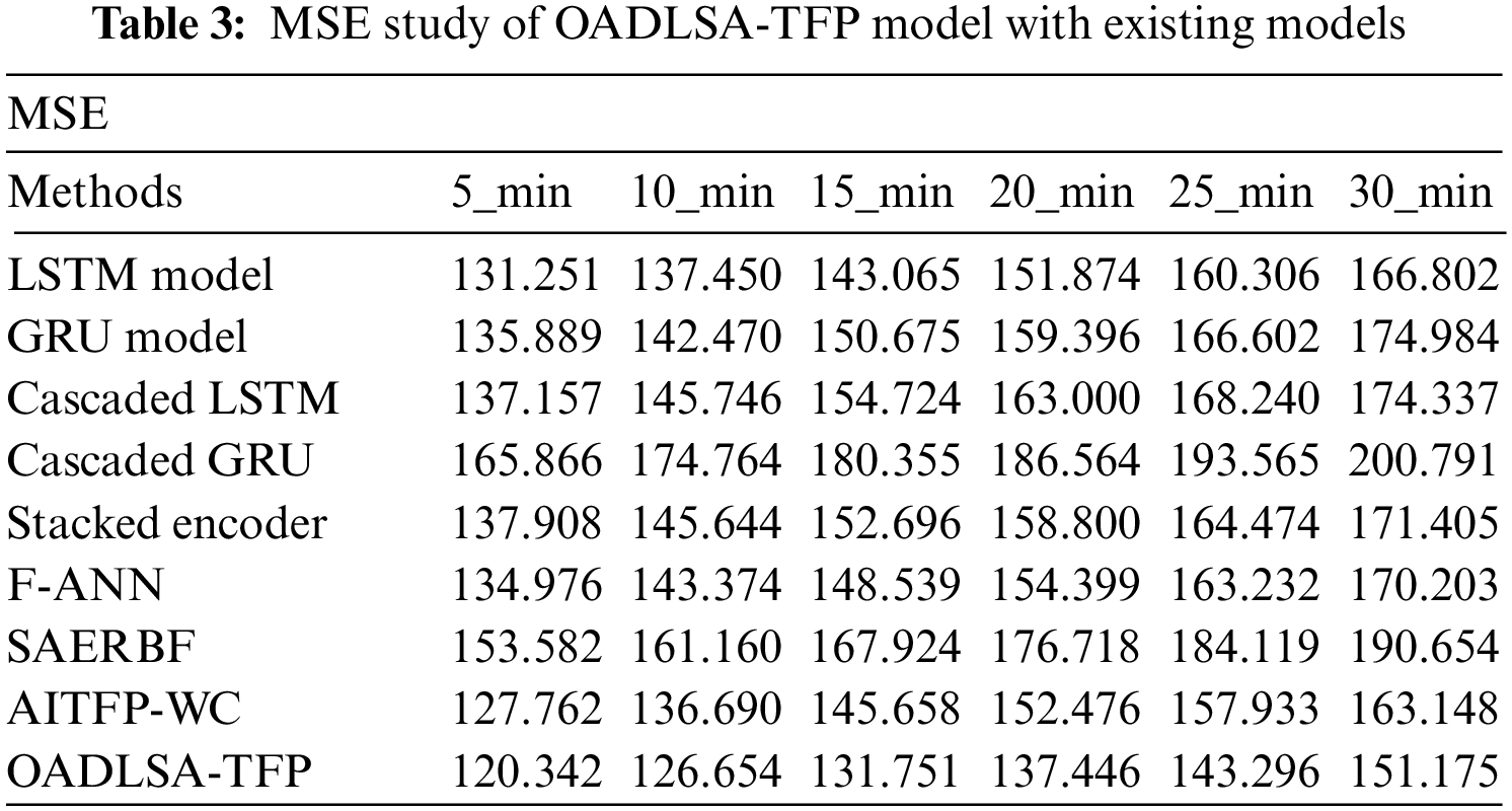
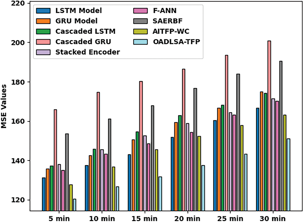
Figure 5: Comparative MSE examination of OADLSA-TFP model under distinct time durations

Similarly, with 10_min, the OADLSA-TFP model has provided least MSE of 126.654. Likewise, with 15_min, the OADLSA-TFP model has gained decreased MSE of 131.751. Moreover, with 20_min, the OADLSA-TFP model has depicted minimum MSE of 137.446. Furthermore, with 30_min, the OADLSA-TFP model has accomplished least MSE of 151.175.

Tab. 4 and Fig. 6 deal with an RMSE inspection of the OADLSA-TFP model with existing ones under distinct durations. The results inferred that the OADLSA-TFP model has revealed enhanced performance with nominal values of RMSE under all-time durations.

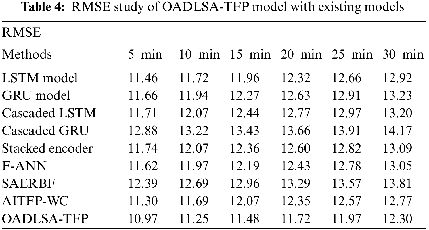
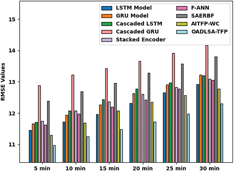
Figure 6: Comparative RMSE examination of OADLSA-TFP model under distinct time durations

For instance, with 5_min, the OADLSA-TFP model has presented reduced RMSE of 10.97. In the same way, with 10_min, the OADLSA-TFP model has provided least RMSE of 11.25. Equally, with 15_min, the OADLSA-TFP model has gained decreased RMSE of 11.48. Also, with 20_min, the OADLSA-TFP model has depicted minimum RMSE of 11.72. Additionally, with 30_min, the OADLSA-TFP model has accomplished least RMSE of 12.30.

Tab. 5 and Fig. 7 deal with a MAPE inspection of the OADLSA-TFP model with existing ones under distinct durations [22,23]. The results inferred that the OADLSA-TFP model has revealed enhanced performance with nominal values of MAPE under all-time durations. For instance, with 5_min, the OADLSA-TFP model has presented reduced MAPE of 8.146%. In the same way, with 10_min, the OADLSA-TFP model has provided least MAPE of 11.195%. Equally, with 15_min, the OADLSA-TFP model has gained decreased MAPE of 14.359%. Also, with 20_min, the OADLSA-TFP model has depicted minimum MAPE of 17.563%. Additionally, with 30_min, the OADLSA-TFP model has accomplished least MAPE of 23.150%.

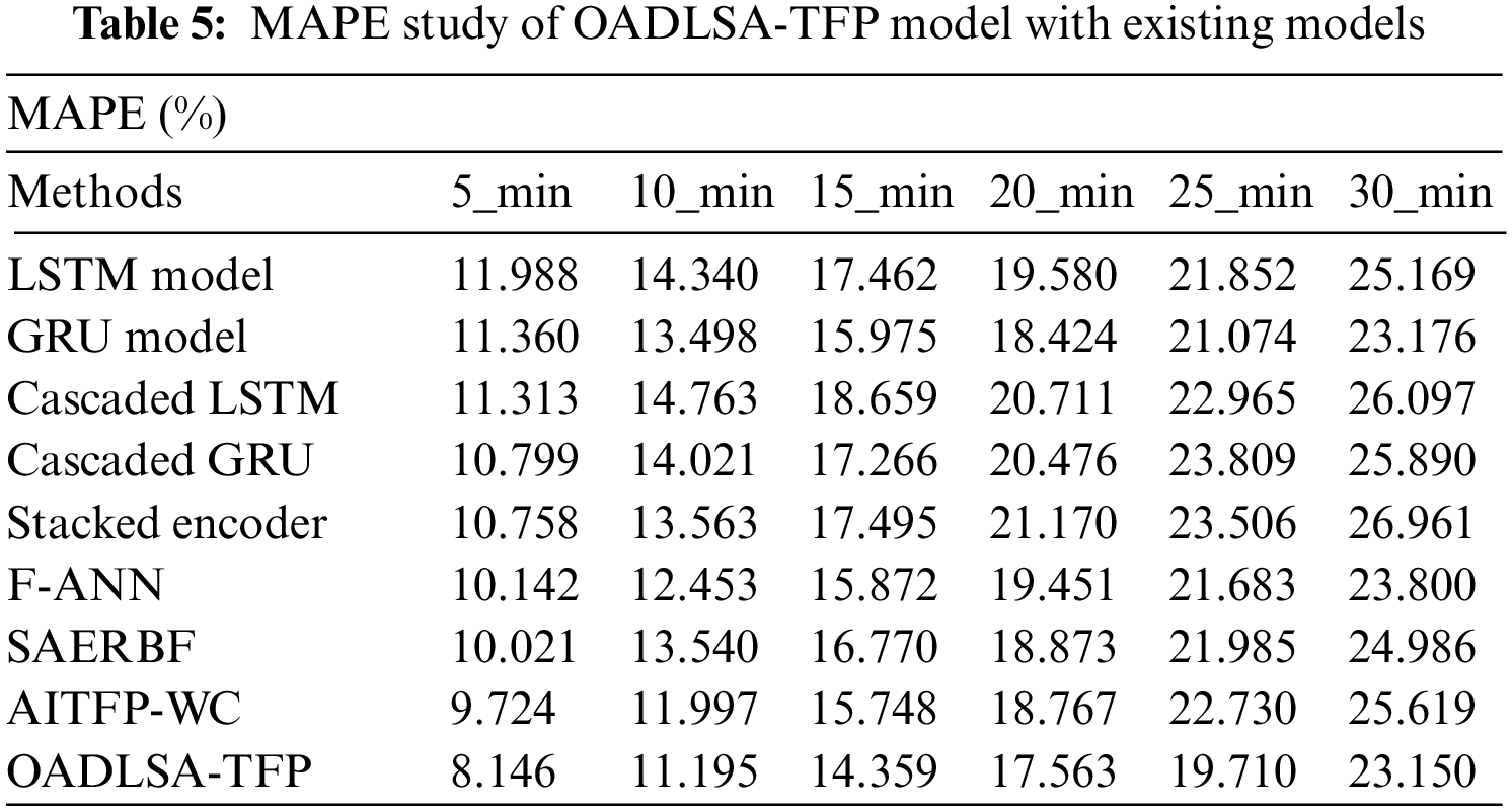
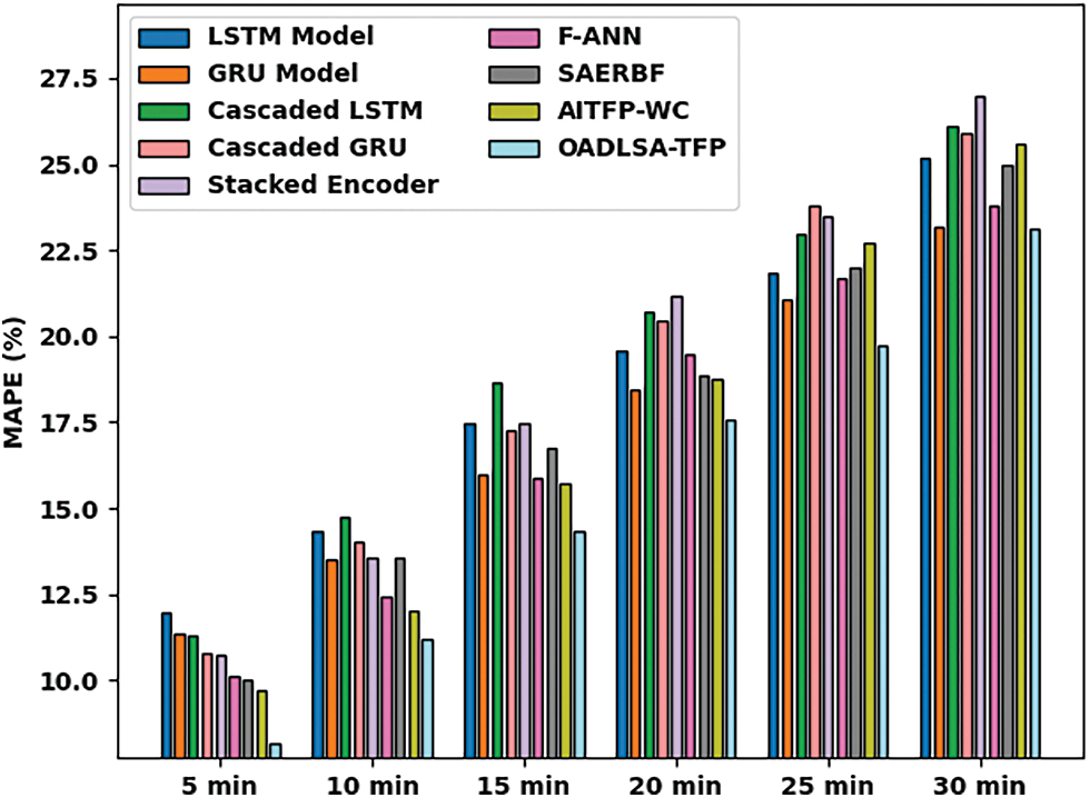
Figure 7: Comparative MAPE examination of OADLSA-TFP model under distinct time durations

By observing the above mentioned tables and figures, it is apparent that the OADLSA-TFP model has resulted in maximum TFP performance over the other methods.

4  Conclusion

In this study, a novel OADLSA-TFP model has been developed to effectually forecast the level of traffic in the environment. The OADLSA-TFP model primarily employed the design of ABLSTM model for predicting traffic flow. In order to enhance the performance of the ABLSTM model, the hyperparameter optimization process is performed using AFSA and thereby boosts the predictive results. A wide-ranging experimental analysis is carried out on benchmark dataset and the obtained values reported the enhancements of the OADLSA-TFP model over the recent approaches. Thus, the OADLSA-TFP model can be used for effective TFP in real time platform. In future, hybrid metaheuristic algorithms can be designed for improved hyperparameter tuning processes.

Acknowledgement: This project was funded by the Deanship of Scientific Research (DSR) at King Abdulaziz University (KAU), Jeddah, Saudi Arabia, under grant no. (G: 665-980-1441). The authors, therefore acknowledge with thanks DSR for technical and financial support.

Funding Statement: This project was funded by the Deanship of Scientific Research (DSR) at King Abdulaziz University (KAU), Jeddah, Saudi Arabia, under grant no. (G: 665-980-1441).

Conflicts of Interest: The authors declare that they have no conflicts of interest to report regarding the present study.

References

 1.  A. Miglani and N. Kumar, “Deep learning models for traffic flow prediction in autonomous vehicles: A review, solutions, and challenges,” Vehicular Communications, vol. 20, no. 2, pp. 100184, 2019. [Google Scholar]

 2.  Y. Wu, H. Tan, L. Qin, B. Ran and Z. Jiang, “A hybrid deep learning based traffic flow prediction method and its understanding,” Transportation Research Part C: Emerging Technologies, vol. 90, no. 2554, pp. 166–180, 2018. [Google Scholar]

 3.  H. Peng, B. Du, M. Liu, M. Liu, S. Ji et al., “Dynamic graph convolutional network for long-term traffic flow prediction with reinforcement learning,” Information Sciences, vol. 578, pp. 401–416, 2021. [Google Scholar]

 4.  C. Ma, G. Dai and J. Zhou, “Short-term traffic flow prediction for urban road sections based on time series analysis and lstm_bilstm method,” IEEE Transactions on Intelligent Transportation Systems, pp. 1–10, 2021. http://dx.doi.org/10.1109/TITS.2021.3055258. [Google Scholar]

 5.  X. Xu, Z. Fang, L. Qi, X. Zhang, Q. He et al., “TripRes: Traffic flow prediction driven resource reservation for multimedia iov with edge computing,” ACM Transactions on Multimedia Computing, Communications, and Applications, vol. 17, no. 2, pp. 1–21, 2021. [Google Scholar]

 6.  W. Li, X. Wang, Y. Zhang and Q. Wu, “Traffic flow prediction over muti-sensor data correlation with graph convolution network,” Neurocomputing, vol. 427, no. 4, pp. 50–63, 2021. [Google Scholar]

 7.  S. Lu, Q. Zhang, G. Chen and D. Seng, “A combined method for short-term traffic flow prediction based on recurrent neural network,” Alexandria Engineering Journal, vol. 60, no. 1, pp. 87–94, 2021. [Google Scholar]

 8.  K. Wang, C. Ma, Y. Qiao, X. Lu, W. Hao et al., “A hybrid deep learning model with 1DCNN-LSTM-Attention networks for short-term traffic flow prediction,” Physica A: Statistical Mechanics and its Applications, vol. 583, no. 12, pp. 126293, 2021. [Google Scholar]

 9.  W. Du, Q. Zhang, Y. Chen and Z. Ye, “An urban short-term traffic flow prediction model based on wavelet neural network with improved whale optimization algorithm,” Sustainable Cities and Society, vol. 69, no. 3, pp. 102858, 2021. [Google Scholar]

10. Y. Qiao, Y. Wang, C. Ma and J. Yang, “Short-term traffic flow prediction based on 1DCNN-LSTM neural network structure,” Modern Physics Letters B, vol. 35, no. 2, pp. 2150042, 2021. [Google Scholar]

11. B. Yang, S. Sun, J. Li, X. Lin and Y. Tian, “Traffic flow prediction using LSTM with feature enhancement,” Neurocomputing, vol. 332, no. 4, pp. 320–327, 2019. [Google Scholar]

12. Y. Liu, J. J. Q. Yu, J. Kang, D. Niyato and S. Zhang, “Privacy-preserving traffic flow prediction: a federated learning approach,” IEEE Internet of Things Journal, vol. 7, no. 8, pp. 7751–7763, 2020. [Google Scholar]

13. X. Chen, H. Chen, Y. Yang, H. Wu, W. Zhang et al., “Traffic flow prediction by an ensemble framework with data denoising and deep learning model,” Physica A: Statistical Mechanics and its Applications, vol. 565, no. 9, pp. 125574, 2021. [Google Scholar]

14. J. Tang, X. Chen, Z. Hu, F. Zong, C. Han et al., “Traffic flow prediction based on combination of support vector machine and data denoising schemes,” Physica A: Statistical Mechanics and its Applications, vol. 534, pp. 120642, 2019. [Google Scholar]

15. Q. Tao, Z. Li, J. Xu, S. Lin, B. D. Schutter et al., “Short-term traffic flow prediction based on the efficient hinging hyperplanes neural network,” IEEE Transactions on Intelligent Transportation Systems, pp. 1–13, 2022. http://dx.doi.org/10.1109/TITS.2022.3142728. [Google Scholar]

16. G. Wu, G. Tang, Z. Wang, Z. Zhang and Z. Wang, “An attention-based BiLSTM-CRF model for chinese clinic named entity recognition,” IEEE Access, vol. 7, pp. 113942–113949, 2019. [Google Scholar]

17. J. Xie, B. Chen, X. Gu, F. Liang and X. Xu, “Self-attention-based BiLSTM model for short text fine-grained sentiment classification,” IEEE Access, vol. 7, pp. 180558–180570, 2019. [Google Scholar]

18. S. Manne, E. L. Lydia, I. V. Pustokhina, D. A. Pustokhin, V. S. Parvathy et al., “An intelligent energy management and traffic predictive model for autonomous vehicle systems,” Soft Computing, vol. 25, no. 18, pp. 11941–11953, 2021. [Google Scholar]

19. K. Shankar, E. Perumal, M. Elhoseny, F. Taher, B. B. Gupta et al., “Synergic deep learning for smart health diagnosis of covid-19 for connected living and smart cities,” ACM Transactions on Internet Technology, vol. 22, no. 3, pp. 16, 1–14, 2022. [Google Scholar]

20. D. K. Jain, Y. Li, M. J. Er, Q. Xin, D. Gupta et al., “Enabling unmanned aerial vehicle borne secure communication with classification framework for industry 5.0,” IEEE Transactions on Industrial Informatics, vol. 18, no. 8, pp. 5477–5484, 2022. [Google Scholar]

21. Y. Feng, S. Zhao and H. Liu, “Analysis of network coverage optimization based on feedback k-means clustering and artificial fish swarm algorithm,” IEEE Access, vol. 8, pp. 42864–42876, 2020. [Google Scholar]

22. M. A. Duhayyim, A. A. Albraikan, F. N. A. Wesabi, H. M. Burbur, M. Alamgeer et al., “Modeling of artificial intelligence based traffic flow prediction with weather conditions,” Computers, Materials & Continua, vol. 71, no. 2, pp. 3953–3968, 2022. [Google Scholar]

23. Y. Hou, Z. Deng and H. Cui, “Short-term traffic flow prediction with weather conditions: Based on deep learning algorithms and data fusion,” Complexity, vol. 2021, pp. 1–14, 2021. [Google Scholar]

This work is licensed under a Creative Commons Attribution 4.0 International License, which permits unrestricted use, distribution, and reproduction in any medium, provided the original work is properly cited.