| Computers, Materials & Continua DOI:10.32604/cmc.2022.030388 | |
| Article |
A Locality-Sensitive Hashing-Based Jamming Detection System for IoT Networks
Computer Science Department, College of Computer and Information Sciences, Imam Mohammad Ibn Saud Islamic University (IMSIU), Riyadh, Saudi Arabia
*Corresponding Author: P. Ganeshkumar. Email: drpganeshkumar@gmail.com
Received: 25 March 2022; Accepted: 01 June 2022
Abstract: Internet of things (IoT) comprises many heterogeneous nodes that operate together to accomplish a human friendly or a business task to ease the life. Generally, IoT nodes are connected in wireless media and thus they are prone to jamming attacks. In the present scenario jamming detection (JD) by using machine learning (ML) algorithms grasp the attention of the researchers due to its virtuous outcome. In this research, jamming detection is modelled as a classification problem which uses several features. Using one/two or minimum number of features produces vague results that cannot be explained. Also the relationship between the feature and the class label cannot be efficiently determined, specifically, if the chosen number of features for training is minimum (say 1 or 2). To obtain good results, machine-learning algorithms are trained by large number of data sets. However, collection of large number of datasets to solve jamming detection is not easy and most of the times generation and collection of large data sets become paradigmatic. In this paper, to solve this problem, more number of features with nominal number of data’s is considered that eases the data collection and the classification accuracy. In this research, an efficient technique based on locality sensitive hashing (LSH) for K-nearest neighbor algorithm (K-NN), which takes less time for constructing and querying the hash table that gives good accuracy is proposed and evaluated. From the results, it is clear that the obtained results are validatable and the model is more sensible.
Keywords: IoT; jamming detection; K-NN; machine learning
IoT is proliferated almost in all areas of engineering and technology to support ease, safe and healthy life in living beings. IoT applications are now being deployed in agriculture, transport, health care, grid, communications, etc. In IoT, sensor/actuators collect information from the environment (where it is deployed) and send them to the centralized server. Sensors/actuators is installed in the environment under study, they send the collected information to the base station and in turn the base station forwards the collected information to a central server for analyzing and decision making. Mostly this setup is realized in wireless networks. Since IoT networks runs on the top of wireless networks, it is susceptible to security attacks. Jamming is most powerful attack in IoT network due to its stealthy behavior. In this paper, an efficient low complexity locality sensitive hashing mechanism based on KNN by applying various network features to differentiate the normal and jammed network is proposed and evaluated.
In the existing literature, mainly jamming detection is carried out based on threshold level of the jamming detection metrics. The nominal quantity of jamming detection metrics such as packet delivery rate (PDR), received signal strength indicator (RSSI) etc is determined by operating the network under normal conditions. To determine the threshold value of the jamming detection metrics during jamming, network is operated under jammed scenario. By examining the threshold value, presence of jamming and absence of jamming can be determined. In the existing literature, this concept of jamming detection is applied in several other numerous forms to detect the jamming attacks. Recently, application of artificial intelligence (AI) technique such as machine learning algorithms and deep learning algorithms for detecting the presence of jamming is carried out successfully in wireless networks, sensor networks. Since the characteristics of sensor network and IoT networks are not same the jamming detection methods that are applied in sensor network cannot be directly applied for IoT networks. Therefore, jamming detection techniques for IoT networks have to be tailored specially according to its characteristics.
The problem of jamming detection in IoT networks in recent days is at its hype because of the inherent vulnerability of IoT networks. The issue of jamming detection based on machine learning algorithms is addressed in many works. The main aim of this paper is to investigate and evaluate the accuracy of the jamming detection by deploying LSH mechanism based on K-NN. For jamming detection based on machine learning, K-NN, decision trees, support vector machines, neural networks, deep neural network are used. K-NN is efficient, easy to use and implement. Currently, the research community is focusing on explainable AI and the important advantage of K-NN is its simplicity to use and explain because the results of K-NN depends upon all the training data points with minimum number of manipulations. So to address jamming detection under explainable AI, K-NN is employed in this paper.
Jamming detection by setting up thresholds (either manually or statistically), jamming detection by using machine learning algorithms are the two most popular techniques for jamming detection, particularly in IoT networks and more generally in wireless networks.
Maximum threshold is set on the jamming detection metrics either manually based on the domain knowledge or statistically by carrying out appropriate statistical test. Setting up threshold is a very tedious task and often threshold are set based on trial and error method to find out the presence of jamming. Threshold setting, often is not a good measure to be used in jamming detection. For threshold setting, samples of PDR, RSSI is collected during the presence and absence of jamming. From the observation, it is identified that the samples collected from the two sets often overlap with each other. Therefore, it is concluded that jamming detection based on threshold setting available in the literature [1], is not suitable for IoT networks. Threshold setting is not holding good even for two metrics, so this cannot be implemented for a jamming detection system which involves with more than two metrics.
ML based JD currently available in the literature exploits only a minimum number of jamming detection metrics. From this, it is clearly understood that jamming detection based on threshold setting and ML based JD on minimum number of metrics is not suitable for sophisticated and rapidly emerging IoT network environment. So the design and implementation of ML based JD with more number of appropriate jamming detection metrics is the need of the hour. This paper focusses on such research unlike the works available in the existing literature [2–4].
An efficient LSH based on K-NN for jamming detection in IoT network using the jamming detection metrics such as PDR, RSSI, packet send ratio (PSR) etc. that varies significantly during jamming is carried out. In this paper, the proposed method is developed, implemented and evaluated for jamming detection in IoT network. Features/jamming detection metrics is used to influence the proposed technique to discover whether the nodes in IoT network is jammed or not. The proposed solution does not incur load on the IoT nodes. Rather, the jamming detection metrics is collected by the IoT gateway and the same is responsible for jamming detection. Therefore, the classification/jamming detection load on the node is negligible.
The output produced by machine learning algorithms are usually hard to make sense out of it. The recent research trend in AI is explainable AI. K-NN is fairly a straight forward algorithm. From the output of K-NN, sufficient clarification can be given based on the majority class. That is, the output can be easily explained/interpreted. Therefore, K-NN based on LSH is employed in this paper. In LSH, the problem of placing the nearest neighbors (NN) is discovered and illustrated in Section 3.3.
In Section 3.6, to avoid the problem of the placement of NN in different bucket, a very simple idea that reduces the time complexity to construct the hash table and to query the hash table is O (m.n.d) and O (m.d) respectively, where m = # hyperplanes, n = # data point vector, d = # dimensions of data point vector.
From the experiments, it is found that K-NN based on LSH cannot be applied to on-the-fly detection. In the existing K-NN based LSH, ‘K’ sets of ‘m’ hyperplanes are constructed and the training time increases with the value of ‘k’. These results are discussed in Section 4.3.
To compare and validate the results from other models, random model is constructed. The range of log loss for cross validation, test data and percentage of in-correctly classified points is extracted and is show cased in Section 4.5.
Finally, in Section 4.6, based on receiver operating characteristics (ROC) curve, it is identified that the performance of the classifier is more sensible.
Numerous jamming detection techniques are available in the literature. Jamming detection can be performed by techniques such as setting up threshold level of the metrics [5–7], application of game theory [8–10], modelling of jamming tolerant systems [11,12], cooperative strategy [13] etc. Recently, jamming detection based on machine learning algorithms are popular [13]. In [14], Cross layer based jamming detection for IoT using artificial intelligence is explored. Jamming detection based on random forest, support vector machine, and neural network for 5G network is carried out in [15]. In [16], ML based jamming detection is carried out for IEEE 802.11. In [17], jamming detection using deep convolutional neural networks and deep recurrent neural network is done for cognitive radio networks. In [18,19], jamming detection for vehicular network is done based on unsupervised machine learning. In [20], ML based jamming detection for cellular mobile network is carried out. Jamming detection for optical network is explored in [21]. Jamming detection for satellite networks is carried out using support vector machine, convolutional neural networks. In [22], ML approach is proposed for jamming detection in unmanned aerial vehicles. In [23,24], ML based jamming detection is performed for wireless ad hoc network. To the best of our knowledge in [25,26], ML based jamming detection is carried out for wireless networks and in [27,28] ML based jamming detection is explored specifically for IoT network. In [29], deep learning is used to mitigate jamming detection in cognitive radio IoT. In [30], the authors explored ML based jamming detection for IoT which is the focus of study in this paper. ML algorithms such as support vector machines, decision trees, K-NN, random forest, real adaboost are used because they are white boxes in which the interpretation of the result is much easy. In this paper unlike in [29], efficient low complexity LSH based K-NN is articulated and implemented. Due to its straight forward design, research in selecting the NN in K-NN is optimized till recently [31]. Because of its simple interpretation and easy implementation, K-NN is still a most used ML algorithms for jamming, intrusion, anomaly detection in different kind of networks [32–36]. In this paper, an efficient LSH based K-NN is developed, deployed and evaluated for jamming detection in IoT networks.
3.1 K-NN Based LSH for Cosine Similarity Theory
The conventional KNN algorithm classifies the test data point by finding the distance between the test data point with every training data point. K nearest neighbors to the training data point is selected and then training data point is classified based on the majority class of the K nearest neighbors. If training data set is huge, then this requires huge number of computations. To alleviate this problem, LSH based KNN is developed. Here the training data points are placed into different buckets. Test data point is placed into a bucket based on its cosine similarity. Then the distance of the training point to the test data point is computed only for the samples that are placed inside the bucket. This method reduces the computations of finding the distance between the test data and all other training data points.
A data point is a multidimensional vector of size d. The distance between any two data points can be determined by various techniques listed in [5–9]. In this paper, cosine similarity is used to figure out the distance between any two data points. The cosine distance between any two data points x1, x2 is the measure of cos of angle between the vectors, θ (x1, x2). Similarly, the similarity between the two vectors x1, x2 can be represented as the difference between one and the cosine distance.
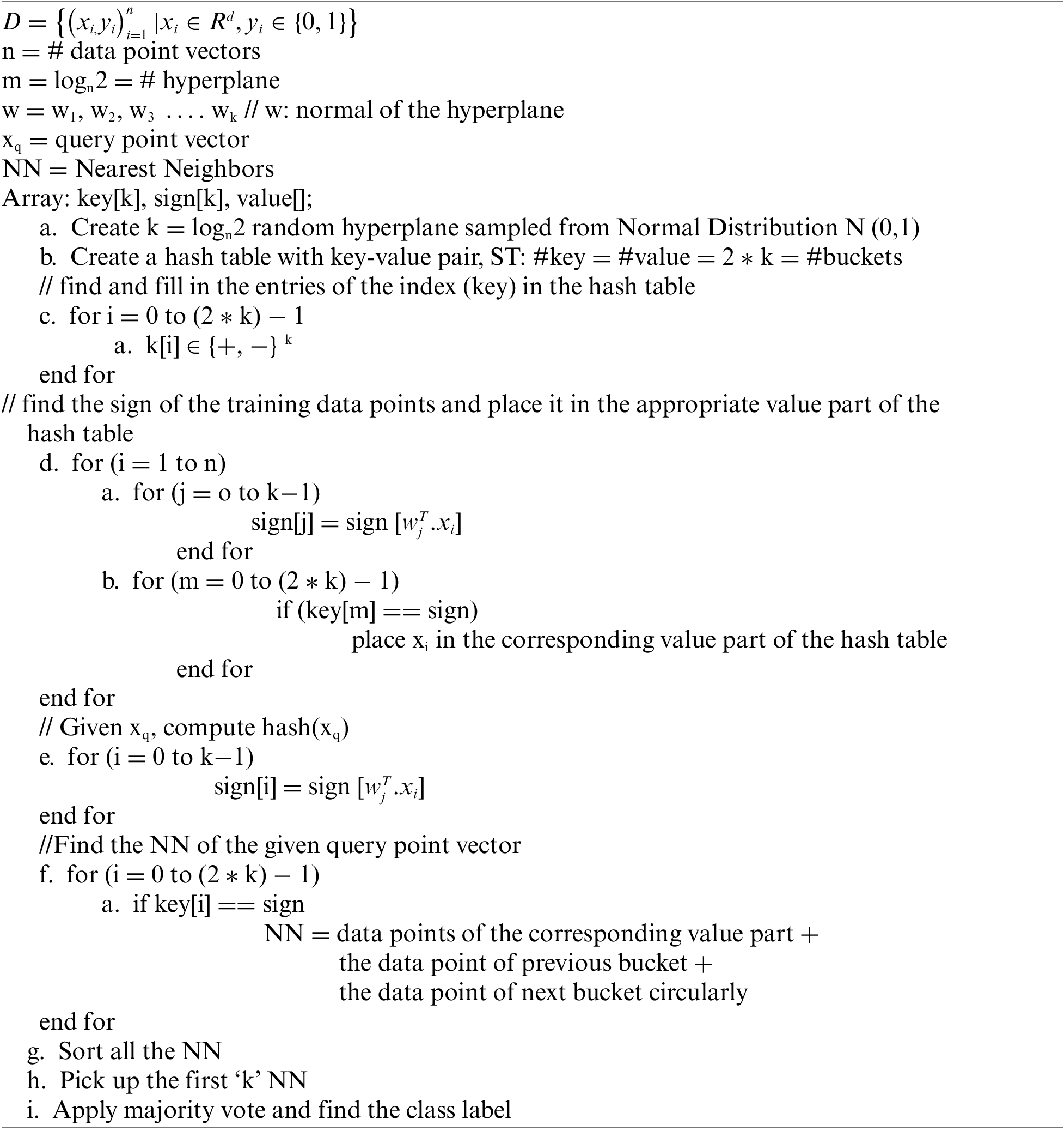
Generate m hyperplane such that m = log n, where n is the total number of training data points.
The following function maps input vectors x1, x2 ∈ Rd to {0, 1}2
hu,v(x1, x2) = (hu(x1),hv(x2)) = [sign(uT x1), sign(v T x2)], where sign (uT x1) returns 1 if (uT x1) ≥ 0, and 0 otherwise, and u and v are from Gaussian distribution
Hash (H) is represented as (r, r (1+ ε), p1, p2) sensitive for θ where r, ε > 0. To prove that the hash is locality sensitive for cosine distance the hash (H) is further represented as
From the above proof it is evident that, the training data set vectors can be placed in the value part of the hash table with its sign in the key part of the hash table. The hash for the query point is calculated as wTxq for all hyperplane and its sign is determined. Based on the sign, the key is identified and the nearest neighbors are retrieved from the value part of the hash table.
• First, make ‘m’ hyperplanes to split the n dimensional feature space into regions and create slices/buckets such that cluster of points lie in a particular slice and be called their neighborhood. Typically m = log (n).
• Next for each point, create a vector (also called hash function) by w1T. xi, where w1 is the hyperplane and xi is the training data vector. Examine w1T. xi if it is greater than 0, it lies on the same side of the hyperplane else other side. Based on that create a vector of size m. For eg, the vector can be [1, −1, −1], denoting point xi lies on same side of normal to hyperplane 1 and opposite side to normal of hyperplane 2 and 3. Now this vector serves as key to the hash table and all the points with the same key or vector representation, will go in to the same bucket as they have similar vector representation denoting that they lie in the neighborhood of each other.
• Now it may happen that two points, which are very close neighbors, could fall on different slice due to the placement of hyperplane and hence not considered as nearest neighbor. To resolve this problem, create L hash tables. In other words, repeat step-2, L times thus creating L hash tables and m random planes L times. Therefore, to classify a query point, compute the hash function L times and get its neighbors from each bucket. Finally, union them and find the nearest neighbors from the list. So in each L iterations, create m hyperplanes. Region splitting and thus vector representation or hash function of the same query point will be different in each of the representations. Due to the placement of different hyperplanes, the hash table will be different because the data points that lied on the same region in previous iteration might lie in a different region in next iteration and vice versa. Time complexity is O (m * d * L) for each query point. Time complexity for creating the hash table is O (m * d * L * n). Space complexity is O(n).
Assume that there exist some random hyperplanes (π1, π2, π3, π4) that passes through the origin in a d-dimensional space (represented by the dataset) and let w1, w2, w3, w4 be the unit normal vector to the hyperplane respectively as depicted in Fig. 1. For illustration purpose, 2-dimensional space (two features) is considered. To generate a hyperplane, d-dimensional vector (‘d’ is the dimension of the dataset) is needed. Random hyperplanes with d-dimensions (2 dimension in illustration example) is generated randomly from normal distribution with mean 0, standard deviation 1.
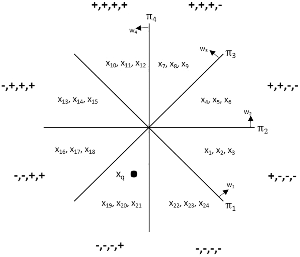
Figure 1: Projection of data points in random hyperplane
As it is shown in the Fig. 1, random hyperplanes passing through origin are considered. Since the vectors of the hyperplane is generated from the normal distribution, the space is divided equally into 8 buckets. For example, consider there are 24 data point vectors in the dataset for simplicity. For illustration purpose, 24 training data vectors (x1…x24) are considered and are placed into its respective buckets as shown in the Fig. 1.
For each training data vector (x), hash is computed: x = h(x), where h(x) is a vector of size ‘m’ that holds the sign of the hyperplane and for training data vector x, wT. x is computed for m hyperplanes, ‘m’ represents the number of hyperplane. Typically, m = log2n. However, here for illustration purpose, n, m is considered to be as 24, 4 respectively. Hash value of the vectors are computed as follows: Assume the training vectors are x1, x2, x3
w1T.x1 = w1T.x2 = w1T.x3 ≥ 0 (sign: +)
w2T.x1 = w2T.x2 = w2T.x3 ≤ 0 (sign: −)
w3T.x1 = w3T.x2 = w3T.x3 ≤ 0 (sign: −)
w4T.x1 = w4T.x2 = w4T.x3 ≤ 0 (sign: −)
The vectors x1, x2, x3 are hashed to the sign (+, −, −, −) and falls into the bucket pointed by the hash (+, −, −, −) as shown in the Fig. 1. Similarly, assume that the hash value of all the training data vectors x4 … x24 are placed in the bucket as demonstrated in Fig. 1.
The hash table is a data structure that is composed of buckets, each of which is indexed by a hash code. Each data vector x is placed into a bucket h(x). Different from the conventional hashing algorithm in computer science that avoids collisions (i.e., avoids mapping two items into same bucket), the hashing approach using a hash table aims to maximize the probability of collision of near items. Given the query q, the items lying in the bucket h(q) are retrieved as near items of q. To improve the recall, L hash tables are constructed, and the items lying in the L (L′, L′ < L) hash buckets h1(q), · · ·, hL(q) are retrieved as near items of q for randomized R-near neighbor search (or randomized approximate R-near neighbor search). To guarantee the precision, each of the L hash codes, needs to be a long code, which means that the total number of the buckets is too large to index directly. Thus, only the nonempty buckets are retained by resorting to conventional hashing of the hash codes hl(x).
The data structure, hash table is represented by two columns called ‘key’, ‘value’. The column ‘key’ contains the hash key and the column ‘value’ contains the NN of the hash key. In the hash table ‘key’ and ‘value’ together constitutes a bucket, where the corresponding NN are placed based on the hash key. Fig. 2, depicts the hash table. Hash function is defined such that it avoids collision. If a query point is given, then the key which is equal to hash of the query point is computed and then this key is used to retrieve the NN corresponding to the key. Given a query data point vector (xq), hash (xq) is calculated and is used as the key in the hash table. The corresponding value part of the hash table contains all the NN.
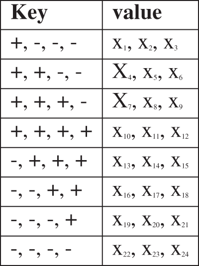
Figure 2: Hash table
For example, consider a query point (xq) as shown in the Fig. 1 Hash (xq) is computed as mentioned above. If key of Hash (xq) = −, −, −, + then the NN, (x19, x20, x21) is retrieved from the corresponding value part of the hash table represented in Fig. 2. The same scenario is also depicted in Fig. 1. The distance of the query vector (xq) to all the NN is computed and sorted in non-decreasing order. Finally, the number of NN based on the hyper parameter ‘K’ is taken from the sorted NN and the class label is determined according to the majority vote.
3.5 Time Complexity of K-NN Based LSH
To construct the hash table, each data point vector has to be multiplied with the each hyperplane. There are ‘m’ hyperplanes and ‘n’ training data point vectors. The dimensionality of training data point vector is ‘d’. So the vector ‘w’ (hyperplane) also has ‘d’ dimensions and thus (mxnxd) multiplications are needed. Therefore, the time complexity to construct hash table = O (m.n.d), where m = # hyperplanes, n = # data point vector, d = # dimensions of data point vector. Typically, number of hyperplane ‘m’ = log2 n, where n = number of training data vector. Therefore, time complexity to query a hash table = O (log2n. d). Given a query point (xq), to find its NN, first key has to computed by performing hash (xq) for all the hyperplanes. There are ‘m’ hyperplanes. So time complexity for finding the key for a given query point is = O (m.d). After finding the key, the NN can be retrieved from the value part of the corresponding key in the hash table. All the NN have to be sorted in ascending order to pick up the ‘k’ NN. Assume that there are ‘i’ NN in the bucket. The time complexity for sorting (merge sort or heap sort) = O (i.log2i). After sorting ‘i’ NN, ‘k’ NN have to be taken in to consideration and a majority vote have to performed to find the class label of the query point. Since the hyper parameter ‘k’ is considered to be very small, time complexity of doing majority vote is O (1). Total time complexity = O (m.d) + O (i.log2 i) + O (1). But the number of NN (number of training data point vector in a bucket), ‘i’ is typically a very small number. Therefore, time complexity to query a hash table = O (m.d), where, m = # hyperplanes, d = dimensionality of training data vector. However, m = log2n. Therefore, time complexity to query a hash table = O (log2n. d).
3.6 Discovering the Placement of Close Data Vectors in Different Bucket and its Solution
In this methodology of finding out the NN, there is a chance to miss out the most appropriate NN, that is, two data point vectors which are originally closer can be put in different adjacent buckets. Due to this, though the two data point vectors are very close to each other in terms of cosine similarity, the placement of the vectors in different adjacent bucket makes them that they are not NN to each other. As shown in the Fig. 3, the data point vector (z1) and the query point (xq) are closer but placed in two different adjacent buckets represented by the key −, −, −, − and −, −, −, + respectively. Hash (xq) results in the key −, −, −, + and so the NN are determined as x19, x20, x21. Here, the NN (z1), which is very closer to (xq) is not taken into consideration as NN. This occurs because the hyperplane π4 separates the placement of the query point (xq) and (z1) to fall into two different adjacent buckets. To overcome this problem, the following algorithm is employed
• ‘k’ sets of ‘m’ random hyperplane is constructed such as h1, h2, … hk
• Find h1(training data vectors) and construct hash table using m random hyperplanes. Find h2(training data vectors) and construct hash table using m random hyperplanes.
• Random hyperplanes used in h1 ≠ random hyperplanes used in h2
• Construct ‘k’ sets of such hyperplanes
• Given a query point (xq), find h1(xq) and its NN called NN1, h2(xq) and its NN called NN2 …. Hk(xq) and its NN called NNk
• Find, NN1 ∪ NN2 …. ∪ NNk and sort all the NN and finally find ‘k’ NN
Due to the construction of k hyperplanes, the probability of the vectors (xq) and (z1), falling into the same hyperplane is high and therefore the placement of two close vectors falling into different bucket can be solved. Since ‘k’ sets of ‘m’ random hyperplane is constructed and due to the presence of ‘n’ training data point vectors of ‘d’ dimensionality, time complexity is (mxnxdxk) multiplications. Time complexity to construct hash table = O (m.n.d.k). Given a query point, since ‘k’ sets of ‘m’ random hyperplane with ‘d’ dimensions are present, (m × d × k) multiplications are required. Therefore, time complexity to query a hash table = O (m.d.k).
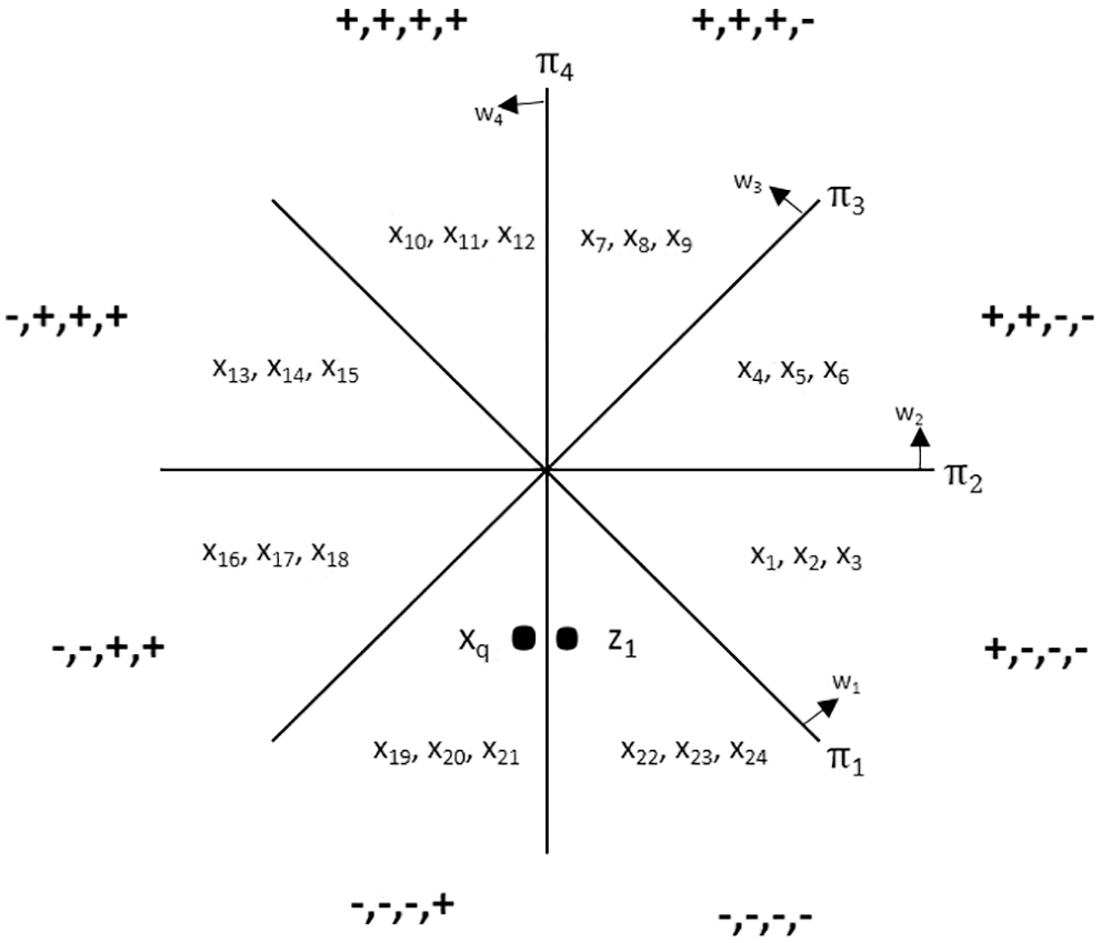
Figure 3: Placement of close data points in different bucket
3.7 Notion of the Proposed Algorithm
To avoid the problem of placing close data vectors in different bucket, in the enhanced version of the algorithm, ‘k’ sets of ‘m’ hyperplanes are constructed. To overcome the problem of the placement of two close data point vectors in different adjacent bucket, consider the scenario shown in the Fig. 4. Bucket with the key (−, −, +, +), (−, −, −, +), (−, −, −, −) contains the data point vectors (x1, x2, x3, z1), (x4, x5, x6, xq), (x7, x8, x9, z1) respectively. If xq is the query point, then hash(xq) will yield the key (−, −, −, +) and the NN in this bucket is (x4, x5, x6). However, on careful examination of Fig. 4, it can be noted that the data point vectors (z1), (z2) are more close to the query point (xq). Since (z1), (z2) are placed in different buckets, though they are close NN, they are not designated as NN. To overcome this issue, the idea explained in the above is proposed. The time complexity of this improved algorithm is O (mxnxdxk). Here k sets of m hyperplane is constructed and for each training data point, k number of hash is computed. This increases the solution time by the factor ‘k’. In addition, the procedure/thumb rule to find the optimal value of ‘k’ is not known and proper literature is not available to determine the value of ‘k’.
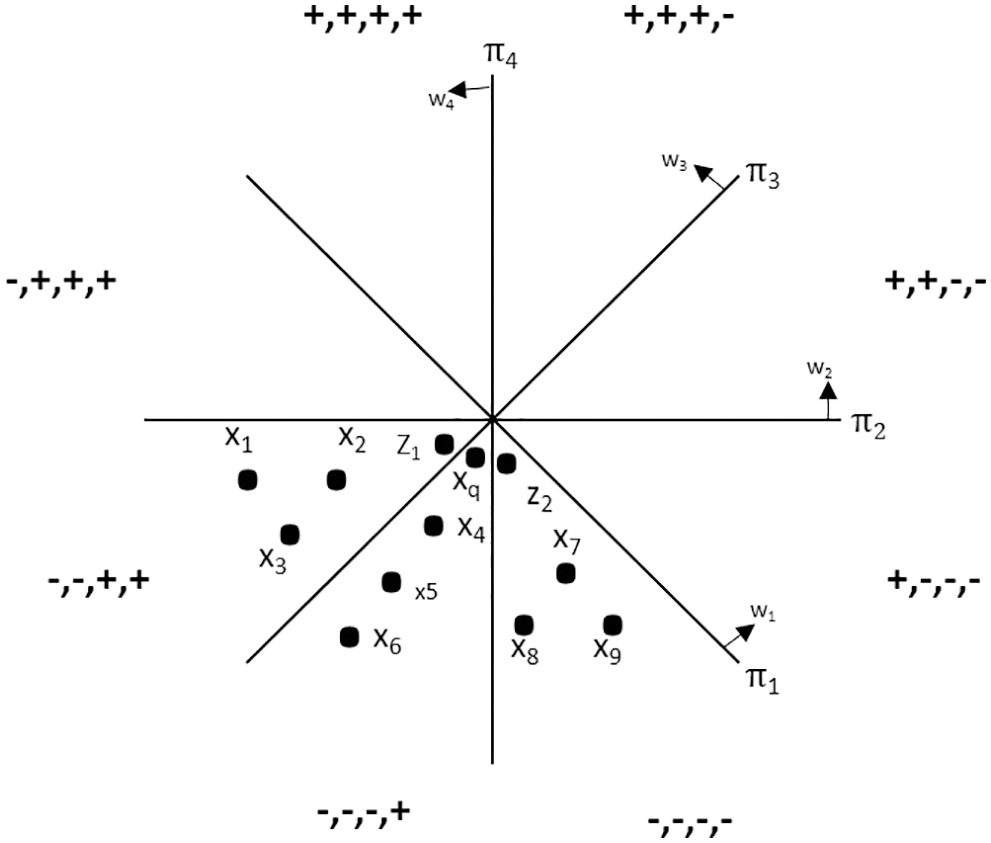
Figure 4: Placement of query point and its NN
In the proposed solution, a simple idea of retrieving the NN is followed. Instead of constructing ‘k’ hyperplane, discussed in Section 3.7, retrieve the NN by computing the key of the query point bucket then include the NN of the bucket which is prior to the query point bucket and the NN of the bucket which is subsequent to the query point bucket. NN = (NN of the bucket which is prior to the query point bucket) + (NN of the query point bucket) + (NN of the bucket which is subsequent to the query point bucket). As it is depicted in Fig. 4, the query point (xq) is present in the bucket (−, −, −, +). NN of the query point is (x4, x5, x6). The bucket which is prior to the bucket (−, −, −, +) is (−, −, +, +) and the bucket which is subsequent to the bucket (−, −, −, +) is (−, −, −, −). According to the proposed algorithm, NN of the bucket prior-to and subsequent-to the query point bucket is included with the NN of the query point bucket. Therefore, NN of the query point bucket is (x1, x2, x3, z1, x4, x5, x6, x7, x8, x9, z1). Here, it can be seen that the vectors (z1), (z2) are now available as the NN of the query point. By using this simple idea, construction of ‘k’ sets of ‘m’ hyperplane is not necessary. Time complexity to construct hash table = O (m.n.d). Time complexity to query a hash table = O (m.d).
Ns-3 jamming model is deployed to prepare the data set. In Ns-3, jamming detection by PDR, Jamming detection by RSSI, jamming detection by PDR and RSSI is available as off the shelf component for study purposes. Variants of jamming detection by using other parameters have to be built as per the user requirements. However, in this paper NS-3 is used to construct network configuration and collect data of various jamming detection metrics.
IoT network with several legitimate nodes N = (n1, n2, …. nl) are considered. Some anchor nodes are deployed randomly that collects the data transmitted by the IoT nodes. For simplicity, the IoT nodes are maintained in static topology. Deliberately, jammer nodes are introduced in the network to jam the data that is transmitted by the IoT nodes. To assure that there is no collision between the data transmitted by the IoT nodes and anchor nodes Wireless-HART protocols is used. The communication channel used is three log distance propagation loss model. The power at the receiver side is calculated by log distance propagation loss model:
4.3 Training Time vs. Hyper Parameter K
Recently, jamming detection on-the-fly is more recommended than the jamming detection that are carried out in off-line mode. Since real time jamming detection is required to exploit its purpose practically to a large extend, it is essential to develop the same [1]. To do such detection, the training time of the data point vectors must be low as possible. Also the training accuracy must not depend on any hyper parameter. In the existing LSH, ‘K’ sets of ‘m’ hyperplanes are constructed and the optimal value of ‘k’ is not available in the literature. An experiment to study the variations of training time with respect to the value of ‘k’ (chosen arbitrarily) is performed. The Fig. 5 shows the training time for the three data sets for each value of ‘k’. It can be noted that, the training time increases with the value of ‘k’. Therefore, it can be concluded that LSH with cosine similarity cannot be applied to on-the-fly detection. As opposed to this, in the proposed system the need for the construction of ‘k’ sets of ‘m’ hyperplane is not required and thus the training time is reduced by 0.65 ms for ‘k’ = 20. Algorithm time of the proposed system is O (m.n.d) as derived in Section 3.6.
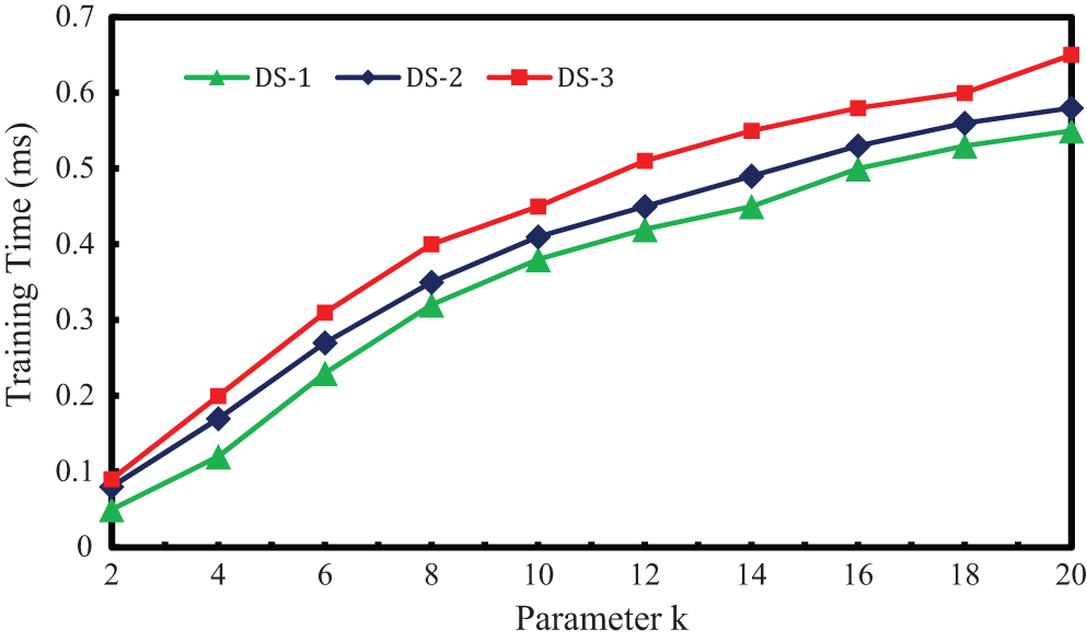
Figure 5: Training time escalation vs. k
To figure out optimum K in K-NN, k fold cross validation is carried out. For this the data set (DS-1) is randomly divided into 60 percent for training, 20 percent for cross validation (for finding the correct value of K) and 20 percent for finding out the performance of the algorithm. But in this approach, only 60 percent of data is used to determine K. So 60 percent training data points and 20 percent of cross validation data points, put together 80 percent of data points is used to figure out K. In this paper, 10-fold cross validation is performed. Algorithm for 10-fold validation cross validation is furnished below. Log loss error is calculated for odd K values (3 to 17), and is plotted as shown in Fig. 6. Log loss uses the actual probability values (lies between 0 to ∞). As it is shown in Fig. 6, for K = 3, log loss error is low and so K = 3 is considered.
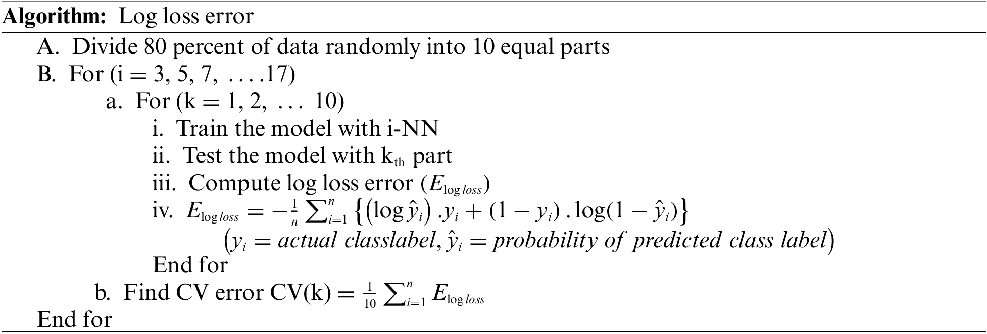
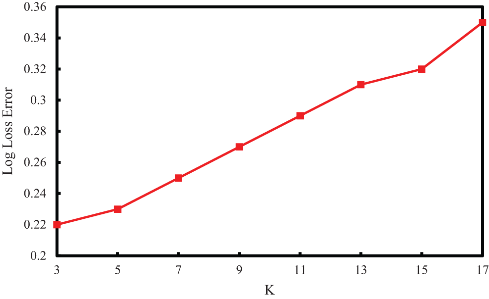
Figure 6: K in K-NN vs. log loss error
The value of log loss varies from (0, ∞), a model with good accuracy has log loss of 0. Finding the worst case log loss is not straight forward. If the worst case log loss is known then by using this value, the performance of the model can be figured out easily. Worst case depends on various parameters such as the feature itself, number of features, number of training data point vector etc. To find out the worst case performance of a model, random model is used. In random model, the probability of data point vector belonging to its class label is generated randomly by using a simple random number generator. Finally, the random number is normalized such that the sum of probability is equal to one. From the results of the random model, the following results are observed. Log loss for cross validation is 3.47. Log loss on test data is 3.31. Percentage of in-correctly classified point is 91.21. From the results, the range of log loss for cross validation, test data and percentage of in-correctly classified points are known. Therefore, this result can be used as a reference to validate the results obtained from other models.
Precision Matrix:
97.3 percent of points are predicted as class + which are actually + and 2.7 percent of points which are actually − are predicted to be as +. 96.2 percent of data points which are actually − are predicted to be as − and 3.8 percent of data points which are actually + is predicted to be as −.
Recall Matrix:
Among the set of all points that belongs to class +, 99.17 percent of data points are predicted to be + and 0.83 percent of points are predicted to be −. Among all the points that belong to −, 97.9 percent of points are predicted to be − and 2.1 percent of points are predicted to be +.
In both precision and recall, the percentage of jammed points (+) that are classified as normal data points is minimum. Therefore, the reliability of the system is more generalizable.
The important metric for binary classification is receiver operating characteristics. Fig. 7 shows ROC curve plotted between true positive rate vs. false positive rate computed at different thresholds. ROC curve can be easily applied to compare the performance of yet another method that is available in the literature or can be used to compare the new algorithm that is going to be emerging in future. The sensitivity can be visualized from the curve. The optimal threshold value can be determined for the classification problem. As shown in the Fig. 7, ROC curve is close to the top left corner which indicate that the performance of the classifier is more sensible.
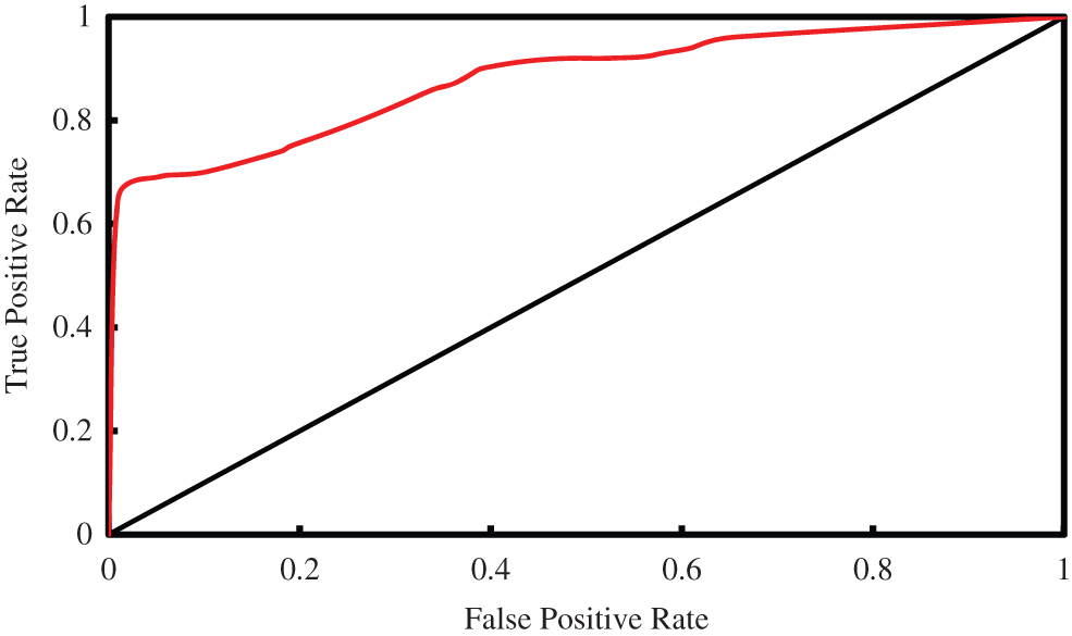
Figure 7: ROC curve
IoT is currently at the top of the hype cycle with investments from companies and venture capital firms. The key areas of research in IoT security includes jamming, authentication, secure routing etc. Though, most of the revenue in IoT comes from the data and not from the devices, the devices have to be protected safely from the vulnerabilities because the IoT devices are the one which is generating the data. Jamming attack surface in IoT is very broad. Jamming can be launched in IoT devices, IoT wireless access technology, IoT Gateway, home LAN, higher layer protocols, cloud, management platform, life cycle management. In the present scenario the IoT devices can self-discover, self-organize, self-configure, self-monitor, self-manage, self-diagnose and self-heal. But because of this open platform, jamming is becoming big challenging task in IoT. Since IoT is emerging field, the researchers and companies are concentrating more on the development of IoT applications and only little amount of work is focused on the security part of the IoT. Jamming detection in IoT network is a big challenge and lot of work is needed to be done in this area in order to safe guard the IoT devices because, the IoT devices are the one which produces the data for information retrieval. In this paper, an efficient technique based on LSH for K-NN is proposed and evaluated. Thereafter, K-NN based LSH for cosine similarity theory, illustration, discovering the placement of close data vectors in different bucket and its solution, efficient K-NN based LSH with reduced time complexity is constructed. Finally the proposed algorithm is evaluated and the results are validated. In this research paper, jamming detection is carried out only on the IoT nodes. In future it is planned to build a holistic jamming detection framework that comprises all the building block of the whole IoT network components: devices, gateway, server, cloud data center, life cycle.
Funding Statement: This research was supported by the Deanship of Scientific Research, Imam Mohammad Ibn Saud Islamic University, Saudi Arabia, Grant number: (20-13-09-004).
Conflicts of Interest: The authors declare that they have no conflicts of interest to report regarding the present study.
References
1. K. P. Vijayakumar, P. Ganeshkumar, M. Anandaraj, K. Selvaraj and P. Sivakumar, “Fuzzy logic-based jamming detection algorithm for cluster-based wireless sensor network,” International Journal of Communication Systems, vol. 31, no. 10, pp. 1–20, 2018. [Google Scholar]
2. P. Ganeshkumar, K. P. Vijayakumar and M. Anandaraj, “A novel jammer detection framework for cluster-based wireless sensor networks,” EURASIP Journal on Wireless Communications and Networking, vol. 2016, no. 1, pp. 1–25, 2016. [Google Scholar]
3. K. P. Vijayakumar, P. Ganeshkumar and M. Anandaraj, “A novel jamming detection technique for wireless sensor networks,” KSII Transactions on Internet and Information Systems (TIIS), vol. 9, no. 10, pp. 4223–4249, 2015. [Google Scholar]
4. O. Osanaiye, A. S. Alfa and G. P. Hancke, “A statistical approach to detect jamming attacks in wireless sensor networks,” Sensors, vol. 18, no. 6, pp. 1691, 2018. [Google Scholar]
5. S. N. Mahapatra, B. K. Singh and V. Kumar, “A survey on secure transmission in internet of things: Taxonomy, recent techniques, research requirements, and challenges,” Arabian Journal for Science and Engineering, vol. 45, no. 8, pp. 6211–6240, 2020. [Google Scholar]
6. A. A. Fadele, M. Othman, I. A. T. Hashem, I. Yaqoob, M. Imran et al., “A novel countermeasure technique for reactive jamming attack in internet of things,” Multimedia Tools and Applications, vol. 78, no. 21, pp. 29899–29920, 2019. [Google Scholar]
7. J. Singh, I. Woungang, S. K. Dhurandher and K. Khalid, “A jamming attack detection technique for opportunistic networks,” Internet of Things, vol. 17, no. 4, pp. 100464, 2021. [Google Scholar]
8. N. Namvar, W. Saad, N. Bahadori and B. Kelley, “Jamming in the internet of things: A game-theoretic perspective,” in Proc. IEEE Global Communications Conf. (GLOBECOM), Washington, DC, USA, pp. 1–6, 2016. [Google Scholar]
9. X. Tang, P. Ren and Z. Han, “Jamming mitigation via hierarchical security game for IoT communications,” IEEE Access, vol. 6, pp. 5766–5779, 2018. [Google Scholar]
10. A. Gouissem, K. Abualsaud, E. Yaacoub, T. Khattab and M. Guizani, “Game theory for anti-jamming strategy in multi-channel slow fading iot networks,” in Proc. of IEEE 7th World Forum on Internet of Things (WF-IoT), New Orleans, Louisiana, USA, pp. 476–481, 2021. [Google Scholar]
11. R. Halloush and H. Liu, “Modeling and performance evaluation of jamming-tolerant wireless systems,” Journal of Ambient Intelligence and Humanized Computing, vol. 10, no. 11, pp. 4361–4375, 2019. [Google Scholar]
12. K. Karoui and F. B. Ftima, “New engineering method for the risk assessment: Case study signal jamming of the m-health networks,” Mobile Networks and Applications, pp. 1–20, 2018. [Google Scholar]
13. N. Ambika, “Tackling jamming attacks in IoT,” in Internet of Things (IoT). Cham: Springer, pp. 153–165, 2020. [Google Scholar]
14. Y. Huo, J. Fan, Y. Wen and R. Li, “A cross-layer cooperative jamming scheme for social internet of things,” Tsinghua Science and Technology, vol. 26, no. 4, pp. 523–535, 2021. [Google Scholar]
15. Y. Arjoune, F. Salahdine, M. S. Islam, E. Ghribi and N. Kaabouch, “A novel jamming attacks detection approach based on machine learning for wireless communication,” in Proc. of the In. Conf. on Information Networking (ICOIN- IEEE), Barcelona, Spain, pp. 459–464, 2020. [Google Scholar]
16. O. Puñal, I. Aktaş, C. J. Schnelke, G. Abidin, K. Wehrle et al., “Machine learning-based jamming detection for IEEE 802.11: Design and experimental evaluation,” in Proc. of the IEEE Int. Symp. on a World of Wireless, Mobile and Multimedia Networks, Sydney, Australia, pp. 1–10, 2014. [Google Scholar]
17. Z. Feng and C. Hua, “Machine learning-based rf jamming detection in wireless networks,” in Proc. of the Third Int. Conf. on Security of Smart Cities, Industrial Control System and Communications (SSIC), Shanghai, China, pp. 1–6, 2018. [Google Scholar]
18. D. Karagiannis and A. Argyriou, “Jamming attack detection in a pair of RF communicating vehicles using unsupervised machine learning,” Vehicular Communications, vol. 13, pp. 56–63, 2018. [Google Scholar]
19. N. V. Abhishek and M. Gurusamy, “JaDe: Low power jamming detection using machine learning in vehicular networks IEEE,” Wireless Communications Letters, vol. 10, no. 10, pp. 2210–2214, 2021. [Google Scholar]
20. S. Sivaprakash and M. Venkatesan, “A design and development of an intelligent jammer and jamming detection methodologies using machine learning approach,” Cluster Computing, vol. 22, no. 1, pp. 93–101, 2019. [Google Scholar]
21. M. Bensalem, S. K. Singh and A. Jukan, “On detecting and preventing jamming attacks with machine learning in optical networks,” in Proc. of IEEE Global Communications Conf. (GLOBECOM-IEEE), Waikoloa, HI, USA, pp. 1–6, 2019. [Google Scholar]
22. R. Morales Ferre, A. de la Fuente, E. S. Lohan, “Jammer classification in GNSS bands via machine learning algorithms,” Sensors, vol. 19, no. 22, pp. 4841–4850, 2019. [Google Scholar]
23. J. Pawlak, Y. Li, J. Price, M. Wright, K. Al Shamaileh et al., “A machine learning approach for detecting and classifying jamming attacks against ofdm-based uavs,” in Proc. of the 3rd ACM Workshop on Wireless Security and Machine Learning, Abudhabi, UAE, pp. 1–6, 2021. [Google Scholar]
24. G. S. Kasturi, A. Jain and J. Singh, “Machine learning-based rf jamming classification techniques in wireless ad hoc networks,” in Proc. of Int. Conf. on Wireless Intelligent and Distributed Environment for Communication, Toronto, Canada, pp. 99–111, 2020. [Google Scholar]
25. G. S. Kasturi, A. Jain and J. Singh, “Detection and classification of radio frequency jamming attacks using machine learning,” Journal of Wireless Mobile Networks Ubiquitous Computing. Dependable Applications, vol. 11, no. 4, pp. 49–62, 2020. [Google Scholar]
26. Z. Feng and C. Hua, “Machine learning-based rf jamming detection in wireless networks,” in Proc. of Third Int. Conf. on Security of Smart Cities, Industrial Control System and Communications (SSIC-IEEE), Shangai, China, pp. 1–6, 2018. [Google Scholar]
27. M. S. Abdalzaher, M. Elwekeil, T. Wang and S. Zhang, “A deep auto encoder trust model for mitigating jamming attack in iot assisted by cognitive radio,” IEEE Systems Journal, pp. 1–11, 2021. [Google Scholar]
28. B. Upadhyaya, S. Sun and B. Sikdar, “Machine learning-based jamming detection in wireless iot networks,” in Proc. of IEEE VTS Asia Pacific Wireless Communications Symp. (APWCS-IEEE), Singapore, pp. 1–5, 2019. [Google Scholar]
29. Y. Wang, Z. Pan and J. Dong, “A new two-layer nearest neighbor selection method for kNN classifier,” Knowledge-Based Systems, vol. 235, no. 1, pp. 107604, 2022. [Google Scholar]
30. H. Sarmadi and A. Karamodin, “A novel anomaly detection method based on adaptive Mahalanobis-squared distance and one-class knn rule for structural health monitoring under environmental effects,” Mechanical Systems and Signal Processing, vol. 140, pp. 106495, 2020. [Google Scholar]
31. F. Kilincer, F. Ertam and A. Sengur, “Machine learning methods for cyber security intrusion detection: Datasets and comparative study,” Computer Networks, vol. 188, pp. 107840, 2021. [Google Scholar]
32. J. Carneiro, N. Oliveira, N. Sousa, E. Maia and I. Praça, “Machine learning for network-based intrusion detection systems: An analysis of the cidds-001 dataset,” in Proc. of Int. Symp. on Distributed Computing and Artificial Intelligence, Italy, pp. 148–158, 2021. [Google Scholar]
33. D. T. Dehkordy and A. Rasoolzadegan, “A new machine learning-based method for android malware detection on imbalanced dataset,” Multimedia Tools and Applications, pp. 1–22, 2021. [Google Scholar]
34. L. Rajesh and P. Satyanarayana, “Evaluation of machine learning algorithms for detection of malicious traffic in scada network,” Journal of Electrical Engineering & Technology, pp. 1–16, 2021. [Google Scholar]
35. B. Mahbooba, R. Sahal, M. Serrano and W. Alosaimi, “Trust in intrusion detection systems: An investigation of performance analysis for machine learning and deep learning models,” Complexity, vol. 2021, no. 3, pp. 1–14, 2021. [Google Scholar]
36. G. Farahani, “Black hole attack detection using k-nearest neighbor algorithm and reputation calculation in mobile ad hoc networks,” Security and Communication Networks, vol. 2021, pp. 1–14, 2021. [Google Scholar]
 | This work is licensed under a Creative Commons Attribution 4.0 International License, which permits unrestricted use, distribution, and reproduction in any medium, provided the original work is properly cited. |