| Computers, Materials & Continua DOI:10.32604/cmc.2022.029221 | |
| Article |
Integrated Evolving Spiking Neural Network and Feature Extraction Methods for Scoliosis Classification
1Faculty of Engineering, Universiti Teknologi Malaysia, School of Computing, Skudai, 81310, Johor, Malaysia
2Faculty of Computer and Mathematical Sciences, Universiti Teknologi MARA Cawangan Melaka Kampus Jasin, Merlimau, 77300, Melaka, Malaysia
3Faculty of Computer and Mathematical Sciences, University Teknologi MARA, Shah Alam, 40450, Selangor, Malaysia
4Fakulti Perubatan & Kesihatan Pertahanan, Universiti Pertahanan Nasional Malaysia (UPNM), Sungai Besi, 57000, Kuala Lumpur, Malaysia
*Corresponding Author: Nurbaity Sabri. Email: nurbaity_sabri@uitm.edu.my
Received: 28 February 2022; Accepted: 20 May 2022
Abstract: Adolescent Idiopathic Scoliosis (AIS) is a deformity of the spine that affects teenagers. The current method for detecting AIS is based on radiographic images which may increase the risk of cancer growth due to radiation. Photogrammetry is another alternative used to identify AIS by distinguishing the curves of the spine from the surface of a human’s back. Currently, detecting the curve of the spine is manually performed, making it a time-consuming task. To overcome this issue, it is crucial to develop a better model that automatically detects the curve of the spine and classify the types of AIS. This research proposes a new integration of ESNN and Feature Extraction (FE) methods and explores the architecture of ESNN for the AIS classification model. This research identifies the optimal Feature Extraction (FE) methods to reduce computational complexity. The ability of ESNN to provide a fast result with a simplicity and performance capability makes this model suitable to be implemented in a clinical setting where a quick result is crucial. A comparison between the conventional classifier (Support Vector Machine (SVM), Multi-layer Perceptron (MLP) and Random Forest (RF)) with the proposed AIS model also be performed on a dataset collected by an orthopedic expert from Hospital Universiti Kebangsaan Malaysia (HUKM). This dataset consists of various photogrammetry images of the human back with different types of Malaysian AIS patients to solve the scoliosis problem. The process begins by pre-processing the images which includes resizing and converting the captured pictures to gray-scale images. This is then followed by feature extraction, normalization, and classification. The experimental results indicate that the integration of LBP and ESNN achieves higher accuracy compared to the performance of multiple baseline state-of-the-art Machine Learning for AIS classification. This demonstrates the capability of ESNN in classifying the types of AIS based on photogrammetry images.
Keywords: Adolescent idiopathic scoliosis; evolving spiking neural network; lenke type; local binary pattern; photogrammetry
Scoliosis is a three-dimensional structural spine deformity characterized by more than ten degrees of lateral curvature. It has been reported that around two to four percent of adolescents suffer from Adolescent Idiopathic Scoliosis (AIS) [1]. Various methods for classifying scoliosis (invasive and non-invasive) have been developed throughout the years. The current and well-known approach of invasive classification is radiographic images. The widely used non-invasive technique is photogrammetry, an alternative to radiographic images [2,3], which is reliable in assessing the shoulder and waist asymmetry in idiopathic scoliosis patients [4,5]. The disadvantage of using radiographic images in classifying scoliosis is that exposure to prolonged radiation can cause the growth of cancer cells [6]. Every patient has a unique form, structure, size, and features [7]. The anthropometric or measurement of body posture is an essential factor in AIS development [8]. Bodily proportions are different according to ethnic diversity [9]. Since Malaysia is a multi-ethnic country, no publicly available Malaysian dataset is present for scoliosis based on photogrammetry. Therefore, this research has created a new dataset consisting of scoliosis images for Malaysia’s multi-ethnic population.
Machine Learning (ML) approaches have been introduced in scoliosis research over the past few years. A comparison between SVM and Deep Learning (DL) was conducted to classify and distinguish between healthy and scoliosis patients from the raster-stereography images [10]. Twenty-seven formetric features were extracted. Both ML models achieved an 80% accuracy rate. A Neural network and SVM classifier were employed to classify normal, toe-in, toe-out, and flat gaits [11]. A hybrid between fast Fourier transform (FFT), principal component analysis (PCA), and linear discriminant analysis (LDA) were applied for FE and dimension reduction. This research achieved over 78% accuracy. SVM is also used to classify between mild and severe gait [12]. Seventy-two gait features were extracted, achieving an 81% accuracy. This further increased to 85.7% using the ReliefF features selection. Classification of the markerless 3D dorsal has been proposed by [13]. In this research, nine shape features and SVM were used to classify the spine with and without deformity, achieving an accuracy of 72.4% and 80%, respectively. RF was utilized to classify spine deformity into 3 classes [14]. Eight descriptors were extracted from the 3D images of spine curvature features, achieving a log loss of 0.5623.
MLP is one of the branches of Artificial Neural Network (ANN) and the most popular neural network model architecture [15]. However, it consists of too many parameters since it is fully connected. Each node is connected to another in a very dense web, resulting in redundancy and inefficiency [16,17]. SVM was first introduced by [18] who was inspired by the statistical learning theory. However, its performance relies on the kernel function. It is crucial to select the appropriate kernel function for a particular classification task to avoid overfitting [19,20]. Leo Breiman proposed RF which is a group of un-pruned classification or regression trees made from the random selection of training data samples [21]. However, the performance of RF can decrease when the data is highly imbalanced. This algorithm takes a relatively longer processing time and is more complex than the Decision Tree (DT) [22,23].
The work of Spiking Neural Network (SNN) began from the observation of the MLP model in which it processes binary spike-based information [24]. As a result, the creation of the SNN model is based on how the MLP model processes information. The ESNN model is an SNN supervised learning model designed to recognize visual patterns. The word “evolving” refers to a shifting repository of output neurons, the weights of which synapses are formed through the network’s supervised learning [25]. Unlike RF and SVM, ESNN trains neurons based on a spike that is only fired if it meets the threshold criteria. If none of the neurons were fired, the extra neurons will evolve during the training phase. The ESNN model demonstrates its simplicity and performance capabilities with its fast one-pass learning algorithm where no data re-training is required. However, determining a suitable parameter value is crucial for ESNN implementation, thus guaranteeing the best output [26]. A comparative study between ESNN, MLP, and SVM has been performed where ESNN achieved a better accuracy of 97.1% on the VidTimit dataset [27–29]. ESNN also exhibited better results compared to MLP, RF, and SVM on the anomaly intrusion dataset [30,31].
Photogrammetric images use the assessment of posture and spinal curvature based on surface examination to determine whether or not a person is suffering from AIS [32]. The surface of the human back consists of a combination of textures and shapes which are extracted from the spine’s curvature. GLCM achieved an accuracy of more than 80% when determining the flexibility of the spine’s curve [33]. LBP has been used to measure spine deformity on scoliosis patients with an accuracy ranging between 84%–91% [34]. SURF identifies the image region (threshold) that shows precise monitoring in the navigated surgery [35]. SIFT is used to automatically detect rib bones in chest X-ray images and successfully addresses the rib-shape variance among patients [36].
From the literature, ESNN performs well compared to other conventional ML techniques. The implementation of ESNN has not yet been conducted in scoliosis research. Due to the promising ability of this ML model, this research proposes an AIS classification model using photogrammetric images with the ESNN classification model. Additionally, the ESNN’s simplicity and performance capabilities make it an ideal model for implementation in clinical settings that requires immediate results. Since they are frequently applied in medical and scoliosis research, this research explores AIS classification based on Malaysian dataset of photogrammetry images using the integration of ESNN with LBP, SIFT, SURF, HOG, and GLCM FE methods.
This research proposed a new classification integration of ESNN and a comparison between five FE methods for the AIS classification model. This research will identify an optimal FE method to improve the computational process. A comparison with the conventional ML model also will be performed with the proposed AIS classification model.
For the ESNN integration, the process begins with the initialization of three important ESNN factors: the modulation factor (Mod), proportion factor (C), and similarity value (Sim) and Receptive Neuron (RN). The parameter value used in this research for Mod, C and Sim is within intervals 0 and 1. Meanwhile, RN is an interval between 20 to 50 where the computational cost increase if it higher. But if it too low, it will affect the performance of ESNN model. Mod is the firing time of presynaptic neuron (j). The function order (j) is the spike rank of the neuron represented by 0, 1, 2, and more, increasing with the firing time (j). The output neuron is produced by the training process in which the similarity distance control by Sim between the weight vectors of the neuron is calculated using Euclidean distance. If the weight vector similarity is high, the neuron will merge. The calculation to merge the neuron is shown in Eq. (1), which includes modifying the weight pattern and the threshold to the average value. N represents the number of samples previously used to update neuron i. Neuron i will be discarded, and the following sample will be processed. However, the neuron value will be added to the repository if the weight vector is a low similarity as a new output neuron.
The Postsynaptic Potential (PSP) fires and becomes disabled only if the threshold value has been reached. Thorpe’s neuron model used in ESNN consists of the one-pass learning algorithm. This stage is important to produce a repository of neurons with a class label. One output sample is expected to be produced by one input sample. However, the output sample is produced based on the weight vector similarity with other output neurons. The PSP (Ui) of neuron i is shown in Eq. (2). Wj represents the presynaptic neuron of j weight. The Ui fires a spike when its potential reaches a certain firing threshold (ft). It is set to a fraction of 0 < C < 1 of a neuron’s maximum potential PSP umax reachable.
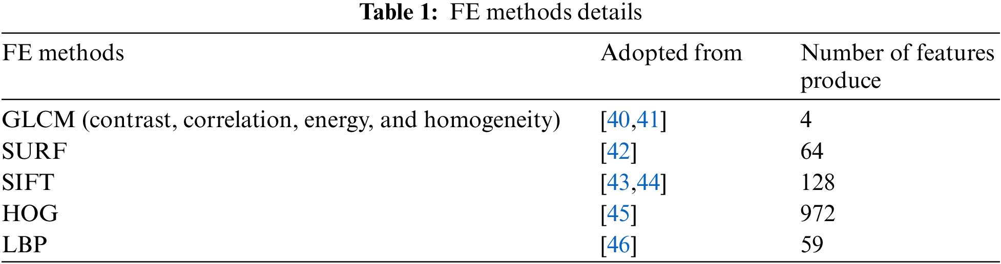
A comparison of five FE methods (GLCM, HOG, LBP, SURF, and SIFT) is performed to identify the optimal FE methods for the classification of Lenke Type 1 (LT1) and Non-Lenke Type 1 (NLT1). Based on the Scoliosis Research Society (SRS), a curve can be divided into two: structural and non-structural. A structural curve bends more than 25 degrees, while a non-structural curve bends less than 25 degrees [37]. Three criteria should be examined regarding the curve of the spine: Proximal Thoracic (PT), Main Thoracic (MT), and Thoracolumbar Lumbar (TL) [38]. This research focuses on Lenke Type 1 (LT1) which consists of only one structural curve (the MT) and non-structural curves (TL and PT). According to [39], LT1 is the most common case in AIS, therefore, this research focuses on LT1. Tab. 1 presents the FE methods applied in this research, the adopted sources, and the number of features produced by each FE method.
Therefore, this research proposes an AIS classification model to classify photogrammetry images into LT1 and NLT1. Experimentation has been conducted on five FE methods. The comparison between three conventional classification models is highlighted in the next subtopic.
This research begins with data collection and pre-processing followed by AIS classification, which is divided into two phases. The proposed model presented in Fig. 1 illustrates how the integration each of the five FE methods with ESNN. Then, the comparison between proposed ESNN and FE methods and conventional classification models, the SVM and RF as in [47]. Meanwhile, second-generation neural network (MLP) as adopted in [48,49].
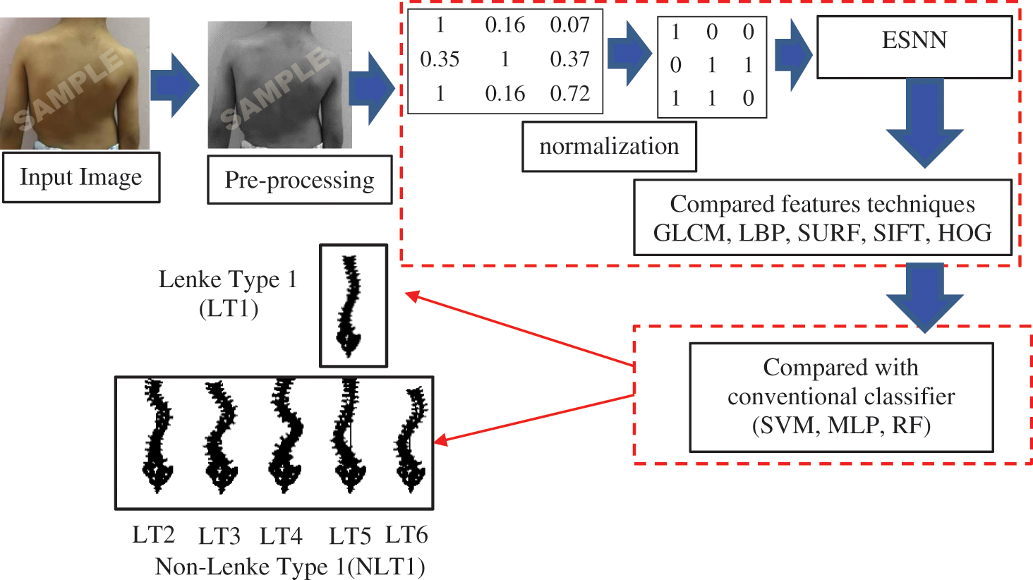
Figure 1: Proposed model architecture for AIS classification based on photogrammetry images
The photogrammetric image acquisition procedure is the pre-operative standard before surgery. In this procedure, the image is of an unclothed human back, standing and facing the wall. In this research, a digital camera is used to take posterior or back view images in a standard control environment. These images were taken by an orthopedic physician from Hospital Universiti Kebangsaan Malaysia (HUKM). Ten images were allocated as Lenke Type 1 and twenty as Lenke Type 2 to Lenke Type 6. Fig. 2 displays some sample images from the dataset used in this research.
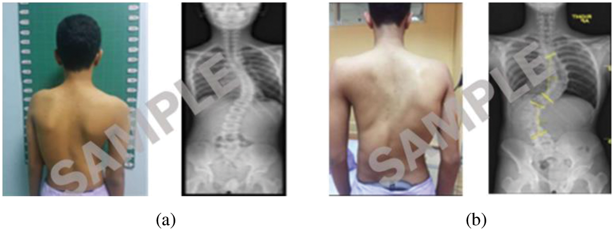
Figure 2: Photogrammetric and radiographic (a) Image of LT1 (b) Image of NLT1
Before further processing, the data must undergo a pre-processing stage where images are resized to 227 × 227 pixels. This is due to the nature of the primary data since it may vary in size. Next, the images are converted to gray-scale before the FE method is applied.
4.3 Propose Integrated ESNN and FE Method
As shown in Fig. 1, the integration between the FE methods (GLCM, LBP, SURF, SIFT, and HOG) has been perform where the optimal FE methods will be selected. This phase applies FE methods to extract features from the coded gray-scale images. The five features produced a list of vectors for each dataset. These features are then normalized to eliminate noise or unnecessary attributes. This process significantly impacts classification performance. Normalization enhances data quality where greater numeric feature values are unable to dominate smaller numeric values [50]. This experiment implements normalization with a range between 0 to 1, as shown in Eq. (3). The mn denotes the normalized value, where max_m is the maximum value of m features. Meanwhile, min_m it represents the minimum values of m features, as shown in Eq. (3).
4.4 Comparison with Convention ML Model
After the normalization process, the normalized vectors are classified by integrating ESNN and FE methods. Evaluation of the performance of the proposed AIS classification model, a comparison between three conventional classifiers (SVM, MLP, RF) perform in this research. In this stage, finding the optimal parameter is essential for each classification model to determine the suitable parameter value used for the AIS classification model. The exploration on the parameter details are discussed in the next subtopic, following the experimental results.
Experiment on integration between ESNN and FE methods perform where the optimal FE methods are identified. A comparison between conventional ML model with propose AIS classification model are evaluated. A few hyper parameters were fine-tuned to obtain optimal classification performance for each ML model. The dataset was divided into 80% training and 20% testing using 10-fold cross-validation. In this experiment, classification accuracy is computed by dividing the number of correctly classified images with the total number of images.
5.1 Evaluation of Proposed Integrated ESNN and FE Methods
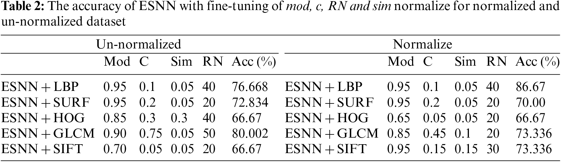
Four essential parameters are used: The Threshold (C), Modulation Factor (Mod), Similarity value (Sim) and Receptive Neuron (RN), where various datasets will have different parameters. Tab. 2 lists the accuracy performances of fine-tuning integration of ESNN with FE methods. From the table, shows the integration of ESNN and LBP achieve a higher accuracy of 86.67% on normalize dataset. Therefore, deep analysis on the accuracy for integration of ESNN and LBP is discussed in this subtopic.
For the integration of ESNN with FE methods, the parameter selected is based on the highest performance accuracy achieved after performing a 10-folds cross-validation. In this experiment, the first parameter is C, where the firing time of the output neuron is observed with a range between [0.05–0.95]. Fig. 3a shows a steady accuracy performance of threshold C from 0.05 until 0.9. The highest performance for C is 0.1, 0.15, 0.25, and 0.3, where the accuracy is 86.67%. A higher value indicates many spikes and a lengthy decision time. Thus, 0.3 is utilized for parameter C. The following parameter is Mod, where the range between [0.05–0.95] has been observed. A better representation of weight patterns according to their output class is obtained when the Mod parameter is set to a high value. Fig. 3b presents an increment accuracy for Mod, where the highest is 0.95. The Mod value should be small as the number of features increases. However, due to the essence of weight calculation, if the Mod value is small, most connections are given the zero-weight value. High modulation signifies that more features are used as input. In this research, features that can be considered small (a Mod of 0.95) achieve the maximum accuracy. The third parameter is Sim, where a range between [0.05–0.95] has been observed in this experiment. High values of the Sim parameter lead to better network architecture. Sim’s value of 0.3 is the best parameter since it achieved the highest accuracy, as shown in Fig. 3c. The number of RN corresponds with the number of firing times. As the number of RN increases, the number of firing times decreases. During the experiment, the observation for RN is between 20, 30, 40 and 50. The low number of neurons affect the performance accuracy. Thus, RN with a value of 40 was utilized in this dataset. Therefore, selecting suitable parameters may influence the achieved results. The experiment shows that 86.67% is achieved for integration of ESNN and LBP by tuning Mod at 0.95, C at 0.3, Sim at 0.3, and RN at 40 for the proposed AIS classification model. The next subtopic discusses the evaluation of FE methods with other conventional ML models.
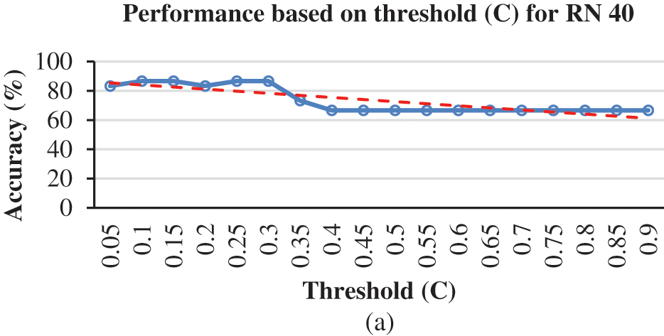
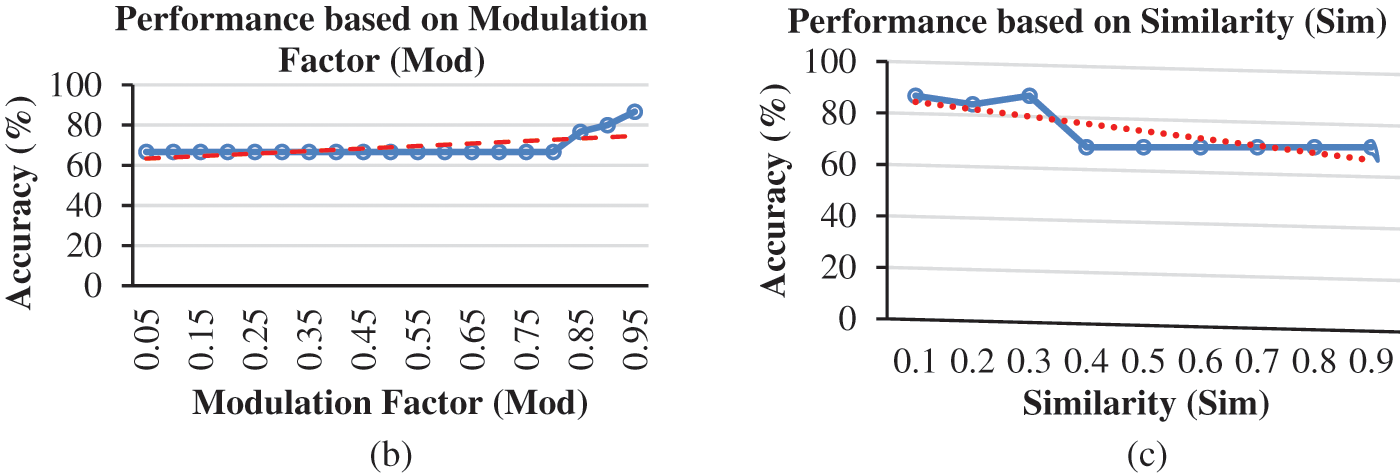
Figure 3: (a) Accuracy based on threshold for LBP + ESNN model, (b) Accuracy based on Modulation Factor (Mod) for LBP and ESNN model and (c) Accuracy based on Similarity (Sim) for LBP and ESNN
5.2 Evaluation for MLP with FE Methods
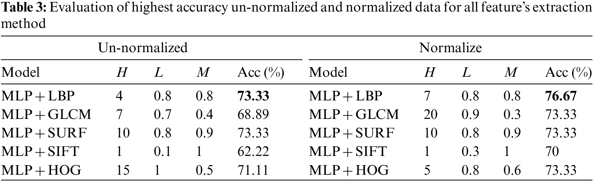
Multilayer perceptions (MLPs) are layered feed forward networks typically trained with static back propagation. To build the MLP model, three hyperparameters are fine-tuned in this research: The Learning rate (L), Momentum rate (M), and Number of hidden layers (H). These hyperparameters are modified to achieve an optimal solution for the model [50]. The number of hidden layers represents a trade-off between performance and the risk of overfitting. The Momentum rate is the value applied to weights during updating, and the learning rate is the amount of weights updated. The accuracy (Acc) was recorded as a benchmark to achieve optimal classification performance. The L and M were adjusted between 0.1 and 1, with one hidden neural net layer. On the other hand, the number of H was adjusted between 1 and 25 [50,51]. From this experiment, the highest accuracy can be listed with the parameter value of H, L, and M. The results of the experiments are shown in Tab. 3 which lists the performance of all FE methods with the MLP model for both the normalized and un-normalized datasets. It can be seen that MLP with LBP presents outstanding results, followed by SURF, for both normalized and un-normalized datasets.
Figs. 4a and 4b display the accuracy for both LBP and SURF using MLP. It can be seen that an increase in the number of hidden layers or number of hidden neurons leads to better classification rate and lower error rate. In Fig. 4a, accuracy is high if the hidden layer is 7 with 0.8 learning rate and 0.8 momentum rate. Accuracy drops if the hidden layer increases. In Fig. 4b, the hidden layers 1, 4, and 6 achieved high accuracy, however, the value drops at layer 7 and beyond. It can therefore be concluded that the optimum values of the hidden layer, momentum rate, and learning rate that achieve the highest accuracy for each FE methods for MLP have been obtained.
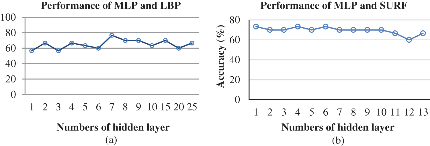
Figure 4: Graphical representation of (a) Performance of MLP and LBP model for every hidden layer with 0.8 learning rate and 0.8 momentum rate. (b) Performance of MLP and LBP model for every hidden layer with 0.3 learning rate and 1 momentum rate
5.3 Evaluation for RF with FE Methods
Three bag sizes of RF (100, 75, and 50) were examined, as adopted in [52]. The bag size determines the number of trees in RF. Bagging is a method of averaging the decision trees. It is in addition to the number of iterations, which is the number of repetitions of the learning process where the previously built model influences the newer model [53]. Fig. 5 illustrates the classification accuracy of RF with three bag sizes. By looking at Fig. 5, we can see that the highest accuracy achieved by RF combined with SURF is 70%.
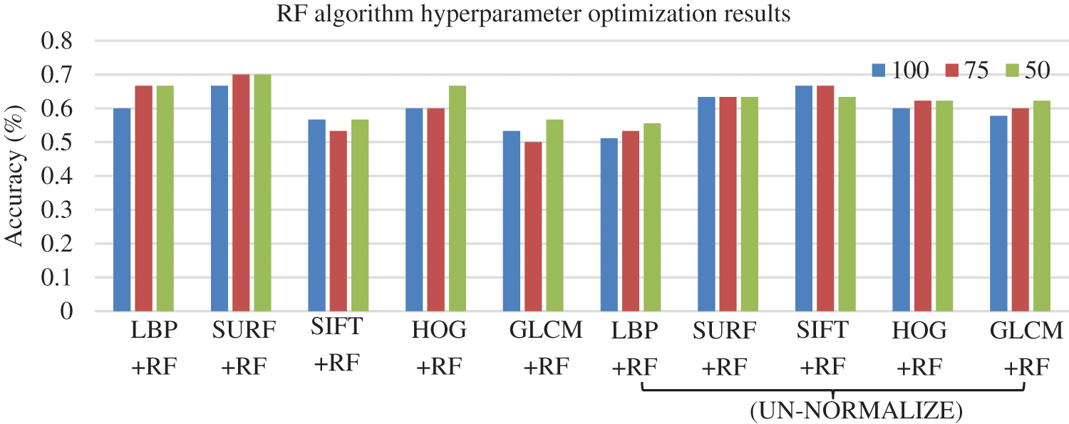
Figure 5: Accuracy results for RF model with different bag sizes based on five FE methods under normalized and un-normalized dataset
5.4 Evaluation for SVM with FE Methods
The SVM algorithm has several kernels. This work used the following: normalized polynomial, linear kernel, Pearson VII (PUK) kernel, and RBF kernel, as adopted in [54,55]. The selection of adequate kernel function was initially made to determine appropriate model configuration. The model that obtains better results is the polynomial kernel with LBP. Both SVM and SURF achieved higher accuracy with normalized polynomial, followed by PUK and RBF. Fig. 6 summarizes the accuracy obtained by the SVM model with four kernels under the normalized and un-normalized datasets. The model that obtained the best results is SVM with polynomial kernel and LBP with an accuracy of 70%. SVM and SURF achieved similar accuracy with normalized polynomial, PUK and RBF.
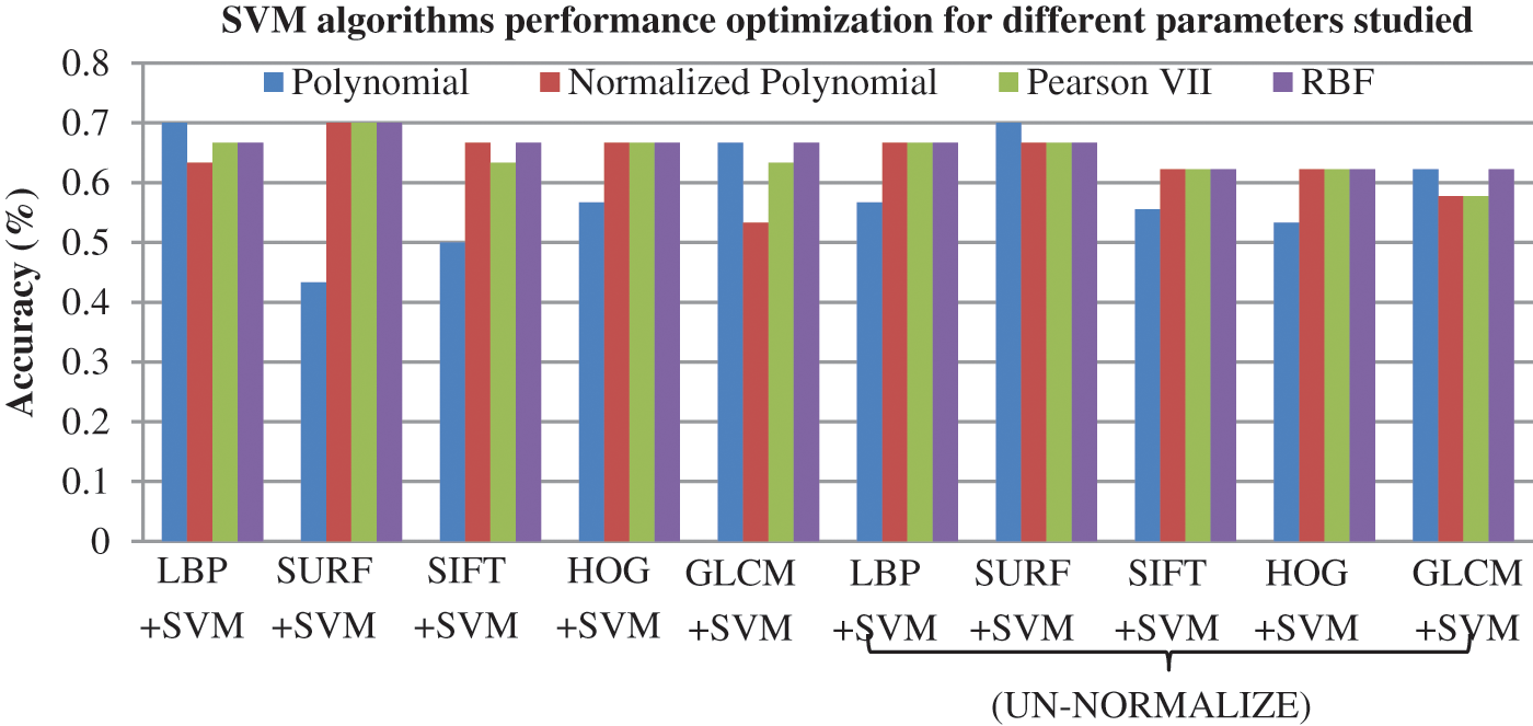
Figure 6: Accuracy results for SVM models with different kernel functions based on five FE methods under normalized and un-normalized dataset
5.5 Performance Summary of all FE Methods with SVM, MLP, RF and ESNN
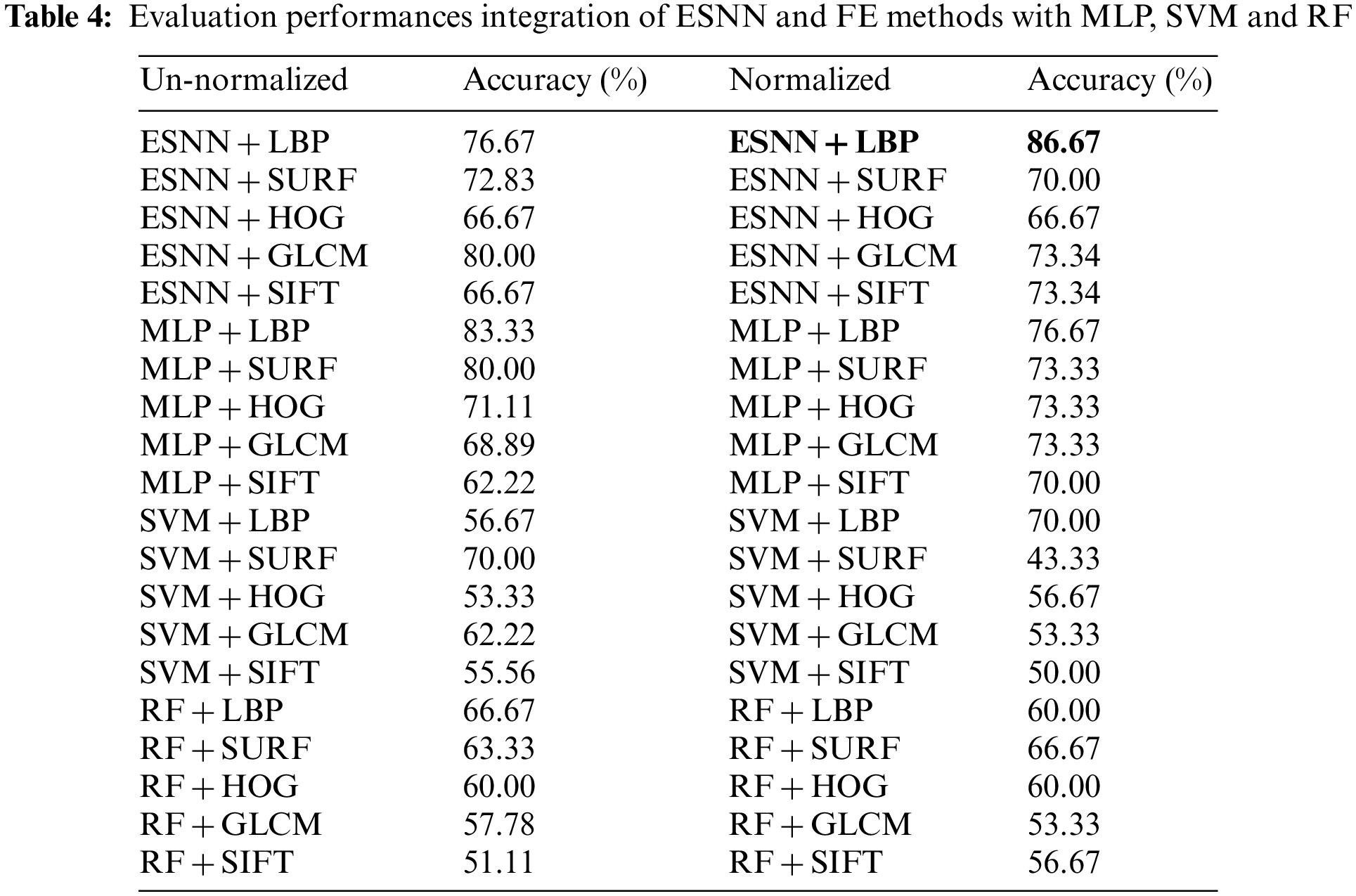
Tab. 4 illustrates the performance comparison of the proposed integration of ESNN and FE methods with convention ML models based on the normalized and un-normalized datasets. The results indicate that the proposed integration of ESNN and LBP has the highest accuracy with 86.67% with a normalized dataset compared to the conventional ML model. This is due to the ability of ESNN to carry visual stimuli information at a single spike [56]. Additionally, the ESNN is capable of adapting to changes in the environment, and its performance is highly dependent on parameter tuning to achieve high accuracy. Besides, the powerful LBP methods based on grayscale and rotation invariant texture operator merge well with ESNN to stimulate a high accuracy result.
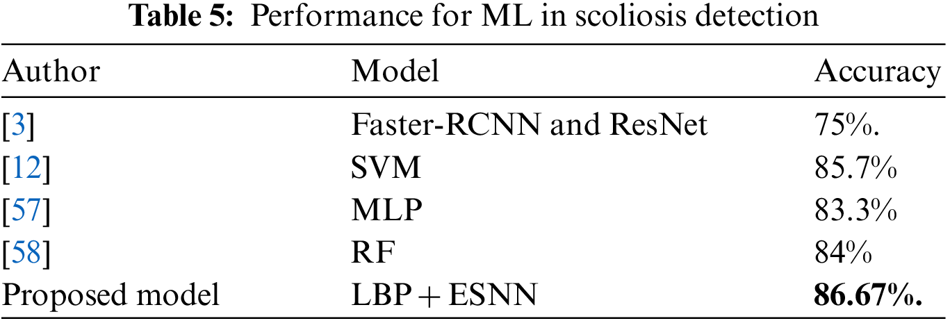
Tab. 5 reveals that the proposed AIS classification model outperforms the conventional ML utilized in scoliosis research. Furthermore, it demonstrates that the research is reliable enough to be employed in clinical settings. The deep learning proposed by [3] achieves 75% accuracy and shows a complex architecture consisting of many layers and requires high computational complexity to process data. The other conventional ML model achieves an accuracy between 83% and 85%. A comparison done on the ESNN model with different ML models shows the ESNN’s ability to achieve high classification accuracy, as mentioned in the literature.
In this research, an AIS classification model based on photogrammetry images was proposed utilizing image processing and a biological plausible algorithm. This is a feasibility study to investigate the FE methods and classification of AIS patients using photogrammetry images. Experimental findings presented an accuracy of 86.67% with the integration of LBP and ESNN models for classification. Comparison between state-of-the-art FE methods (LBP, GLCM, HOG, SURF, and SURF) with conventional ML models (SVM, MLP, and RF) exhibit the potential of the proposed integration of ESNN and LBP for AIS classification. This can complement conventional radiographic techniques since they contribute to cancer, thereby affecting AIS patients. The proposed model classifies the Lenke type at high accuracy to assist orthopedic physicians in choosing the appropriate treatment. In future, more data on photogrammetry images of the human back will be obtained from hospitals throughout Malaysia. Currently, there are a few hospitals that actively provide scoliosis treatment. More experiments will be conducted to develop AIS classification model using photogrammetry images by enhancing the integration of LBP-ESNN with the introduction of the feature reduction algorithm to improve the current accuracy, as adopted in [59].
Acknowledgement: This work is supported by the Ministry of Education Malaysia and Universiti Teknologi Malaysia through Research University Grant Scheme (Q.J130000.2651.16J63), the data collection from Hospital University of Kebangsaan Malaysia.
Funding Statement: This work is supported by the Ministry of Education Malaysia and Universiti Teknologi Malaysia through Research University Grant Scheme (Q.J130000.2651.16J63).
Conflicts of Interest: The authors declare that they have no conflicts of interest to report regarding the present study.
References
1. S. Haleem and C. Nnadi, “Scoliosis: A review,” Paediatrics and Child Health (United Kingdom), vol. 28, no. 5, Churchill Livingstone, pp. 209–217, 2018. [Google Scholar]
2. I. J. Rodrigues, C. T. Candotti, T. S. Furlanetto, V. H. Dutra, M. A. do Amaral et al., “Validation of a mathematical procedure for the cobb angle assessment based on photogrammetry,” Journal of Chiropractic Medicine, vol. 18, pp. 270–277, 2019. [Google Scholar]
3. J. Yang, K. Zhang, H. Fan, Z. Huang, Y. Xiang et al., “Development and validation of deep learning algorithms for scoliosis screening using back images,” Communications Biology, vol. 2, no. 1, pp. 1–8, 2019. [Google Scholar]
4. R. M. C. Aroeira, E. B. de Las Casas, A. E. M. Pertence, M. Greco and J. M. R. S. Tavares, “Non-invasive methods of computer vision in the posture evaluation of adolescent idiopathic scoliosis,” Journal of Bodywork and Movement Therapies, vol. 20, no. 4, Churchill Livingstone, pp. 832–843, 2016. [Google Scholar]
5. J. Bago, J. Pizones, A. Matamalas and E. D’agata, “Clinical photography in severe idiopathic scoliosis candidate for surgery: Is it a useful tool to differentiate among Lenke patterns?” European Spine Journal, vol. 28, pp. 3018–3025, 2019. [Google Scholar]
6. A. R. Levy, M. S. Goldberg, N. E. Mayo, J. A. Hanley and B. Poitras, “Reducing the lifetime risk of cancer from spinal radiographs among people with adolescent idiopathic scoliosis,” Spine, vol. 21, no. 13, pp. 1540–1547, 1996. [Google Scholar]
7. S. P. Yadav and S. Yadav, “Image fusion using hybrid methods in multimodality medical images,” Medical & Biological Engineering & Computing, vol. 58, no. 4, pp. 669–687, 2020. [Google Scholar]
8. E. Matusik, J. Durmala and P. Matusik, “Association of body composition with curve severity in children and adolescents with Idiopathic Scoliosis (IS),” Nutrients, vol. 8, no. 2, pp. 71, 2016. [Google Scholar]
9. K. Karmegam, S. M. Sapuan, M. Y. Ismail, N. Ismail, M. S. Bahri et al., “Anthropometric study among adults of different ethnicity in Malaysia,” International Journal of Physical Sciences, vol. 6, no. 4, pp. 777–788, 2011. [Google Scholar]
10. T. Colombo, M. Mangone, A. Bernetti, M. Paoloni, V. Santilli et al., “Supervised and unsupervised learning to classify scoliosis and healthy subjects based on non-invasive rasterstereography analysis,” PLoS One, vol. 16, no. 12, pp. 1–24, 2019. [Google Scholar]
11. X. Linghui, J. Chen, W. Fei, C. Yuting, Y. Wei et al., “Machine-learning-based children’s pathological gait classification with low-cost gait-recognition system,” BioMedical Engineering OnLine, vol. 20, no. 1, pp. 1–19, 2021. [Google Scholar]
12. J. S. Cho, Y. S. Cho, S. B. Moon, M. J. Kim, H. D. Lee et al., “Scoliosis screening through a machine learning based gait analysis test,” International Journal of Precision Engineering and Manufacturing, vol. 19, no. 12, pp. 1861–1872, 2018. [Google Scholar]
13. J. Arivudaiyanambi, G. Renganathan and S. Cukovic, “Classification of markerless 3D dorsal shapes in adolescent idiopathic scoliosis patients using machine learning approach,” in 2021 IEEE Int. Biomedical Instrumentation and Technology Conf. (IBITeC), Yogyakarta, Indonesia, pp. 83–87, 2021. [Google Scholar]
14. E. García-Cano, F. Arambula Cosio, L. Duong, C. Bellefleur, M. Roy-Beaudry et al., “Dynamic ensemble selection of learner-descriptor classifiers to assess curve types in adolescent idiopathic scoliosis,” Medical & Biological Engineering & Computing, vol. 56, no. 12, pp. 2221–2231, 2018. [Google Scholar]
15. H. I. Dino and M. B. Abdulrazzaq, “Facial expression classification based on SVM, KNN and MLP classifiers,” in 2019 Int. Conf. on Advanced Science and Engineering (ICOASE), University of Zakho, Duhok Polytechnic University, Kurdistan Region, Iraq, pp. 70–75, 2019. [Google Scholar]
16. A. Ganatra and D. Panchal, “Behaviour analysis of multilayer perceptronswith multiple hidden neurons and hidden layers,” International Journal of Computer Theory and Engineering, vol. 3, no. 2, pp. 332–337, 2011. [Google Scholar]
17. B. Turkoglu and E. Kaya, “Training multi-layer perceptron with artificial algae algorithm,” Engineering Science and Technology, an International Journal, vol. 23, no. 6, pp. 1342–1350, 2020. [Google Scholar]
18. V. N. Vapnik, “An overview of statistical learning theory,” IEEE Transactions on Neural Networks, vol. 10, no. 5, pp. 988–999, 1999. [Google Scholar]
19. C. J. C. Burges, “A tutorial on support vector machines for pattern recognition,” Data Mining and Knowledge Discovery, vol. 2, no. 2, pp. 121–167, 1998. [Google Scholar]
20. A. Serra, P. Galdi and R. Tagliaferri, “Machine learning for bioinformatics and neuroimaging,” Wiley Interdisciplinary Reviews: Data Mining and Knowledge Discovery, vol. 8, no. 5, pp. 1–33, 2018. [Google Scholar]
21. L. Breiman, “Random forests,” Machine Learning, vol. 45, no. 1, pp. 5–32, 2001. [Google Scholar]
22. T. M. Berhane, C. R. Lane, Q. Wu, B. C. Autrey, O. A. Anenkhonov et al., “Decision-tree, rule-based, and random forest classification of high-resolution multispectral imagery for wetland mapping and inventory,” Remote Sensing, vol. 10, no. 4, pp. 580, 2018. [Google Scholar]
23. E. Yuk, S. Park, C. S. Park and J. G. Baek, “Feature-learning-based printed circuit board inspection via speeded-up robust features and random forest,” Applied Sciences, vol. 8, no. 932, pp. 1–14, 2018. [Google Scholar]
24. A. Sengupta, Y. Ye, R. Wang, C. Liu and K. Roy, “Going deeper in spiking neural networks: VGG and residual architectures,” Frontiers in Neuroscience, vol. 13, no. 95, pp. 1–10, 2019. [Google Scholar]
25. S. Schliebs and N. Kasabov, “Evolving spiking neural network-A survey,” Evolving Systems, vol. 4, no. 2, pp. 87–98, 2013. [Google Scholar]
26. A. Saleh, S. Shamsuddin and H. Hamed, “Multi-objective differential evolution of evolving spiking neural networks for classification problems,” in IFIP Int. Conf. on Artificial Intelligence Applications and Innovations, Bayonne, France, pp. 351–368, 2015. [Google Scholar]
27. S. G. Wysoski, L. Benuskova and N. Kasabov, “Evolving spiking neural networks for audiovisual information processing,” Neural Networks, vol. 23, no. 7, pp. 819–835, 2010. [Google Scholar]
28. S. G. Wysoski, L. Benuskova and N. Kasabov, “Fast and adaptive network of spiking neurons for multi-view visual pattern recognition,” Neurocomputing, vol. 71, no. 13–15, pp. 2563–2575, 2008. [Google Scholar]
29. S. G. Wysoski, L. Benuskova and N. Kasabov, “On-line learning with structural adaptation in a network of spiking neurons for visual pattern recognition,” in Int. Conf. on Artificial Neural Networks, 2006, pp. 61–70, 2006. [Google Scholar]
30. K. Demertzis and L. Iliadis, “A hybrid network anomaly and intrusion detection approach based on evolving spiking neural network classification,” International Conference on e-Democracy, vol. 441, pp. 11–23, 2013. [Google Scholar]
31. T. Ibad, A. Kadir, N. Binti and A. B. Aziz, “Evolving spiking neural network: A comprehensive survey of its variants and their results,” Journal of Theoretical and Applied Information Technology, vol. 31, no. 24, pp. 4061–4081, 2020. [Google Scholar]
32. A. P. G. Castro, J. D. Pacheco, C. Lourenco, S. Queiros, A. H. J. Moreira et al., “Evaluation of spinal posture using microsoft KinectTM: A preliminary case-study with 98 volunteers,” Porto Biomedical Journal, vol. 2, no. 1, pp. 18–22, 2017. [Google Scholar]
33. C. Chevrefils, D. Perie, S. Parent and F. Cheriet, “To distinguish flexible and rigid lumbar curve from mri texture analysis in adolescent idiopathic scoliosis: A feasibility study,” Journal of Magnetic Resonance Imaging, vol. 48, no. 1, pp. 178–187, 2018. [Google Scholar]
34. F. Berton, F. Cheriet, M. C. Miron and C. Laporte, “Segmentation of the spinous process and its acoustic shadow in vertebral ultrasound images,” Computers in Biology and Medicine, vol. 72, pp. 201–211, 2016. [Google Scholar]
35. F. Manni, A. Elmi-Terander, G. Burstrom, O. Persson, E. Edstrom et al., “Towards optical imaging for spine tracking without markers in navigated spine surgery,” Sensors, vol. 20, no. 13, pp. 3641, 2020. [Google Scholar]
36. S. Candemir, S. Jaeger, S. Antani, U. Bagci, L. R. Folio et al., “Atlas-based rib-bone detection in chest X-rays,” Computerized Medical Imaging and Graphics, vol. 51, pp. 32–39, 2016. [Google Scholar]
37. C. Slattery and K. Verma, “Classifications in brief: The lenke classification for adolescent idiopathic scoliosis,” Clinical Orthopaedics and Related Research, vol. 476, no. 11, pp. 2271, 2018. [Google Scholar]
38. L. G. Lenke, R. R. Betz, T. R. Haher, M. A. Lapp, A. A. Merola et al., “Multisurgeon assessment of surgical decision-making in adolescent idiopathic scoliosis: Curve classification, operative approach, and fusion levels,” Spine, vol. 26, no. 21, pp. 2347–2353, 2001. [Google Scholar]
39. D. Kargin, I. Turk, A. Albayrak, I. Avni Bayhan and A. Kaygusuz, “Change of sagittal spinopelvic parameters after selective and non-selective fusion in lenke type 1 adolescent idiopathic scoliosis patients,” Turkish Neurosurgery, vol. 29, no. 1, pp. 77–82, 2019. [Google Scholar]
40. F. Yang, M. Hamit, C. B. Yan, J. Yao, A. Kutluk et al., “Feature extraction and classification on esophageal X-ray images of xinjiang kazak nationality,” Journal of Healthcare Engineering, vol. 2017, pp. 1–11, 2017. [Google Scholar]
41. A. A. Chandini and B. U. Maheswari, “Improved quality detection technique for fruits using GLCM and multiclass SVM,” in 2018 Int. Conf. on Advances in Computing, Communications and Informatics, ICACCI 2018, Bangalore, India, pp. 150–155, 2018. [Google Scholar]
42. H. Bay, T. Tuytelaars and L. Van Gool, “SURF: Speeded up robust features,” In European Conference on Computer Vision, pp. 404–417, 2006. [Google Scholar]
43. D. G. Lowe, “Distinctive image features from scale-invariant keypoints,” International Journal of Computer Vision, vol. 60, no. 2, pp. 91–110, 2004. [Google Scholar]
44. M. Kasiselvanathan, V. Sangeetha and A. Kalaiselvi, “Palm pattern recognition using scale invariant feature transform,” International Journal of Intelligence and Sustainable Computing, vol. 1, no. 1, pp. 44–52, 2020. [Google Scholar]
45. N. Dalal and B. Triggs, “Histograms of oriented gradients for human detection,” in Proc.-2005 IEEE Computer Society Conf. on Computer Vision and Pattern Recognition, CVPR 2005, San Diego, CA, USA, vol. 1, pp. 886–893, 2005. [Google Scholar]
46. T. Ojala, M. Pietikäinen and T. Mäenpää, “Gray scale and rotation invariant texture classification with local binary patterns,” European Conference on Computer Vision, vol. 1842, pp. 404–420, 2000. [Google Scholar]
47. I. Ahmad, M. Basheri, M. J. Iqbal and A. Rahim, “Performance comparison of support vector machine, random forest, and extreme learning machine for intrusion detection,” IEEE Access, vol. 6, pp. 33789–33795, 2018. [Google Scholar]
48. D. Morariu, R. Cretulescu and M. Breazu, “The weka multilayer perceptron classifier,” International Journal of Advanced Statistics and IT&C for Economics and Life Sciences, vol. 7, no. 1, pp. 16–19, 2017. [Google Scholar]
49. X. Zhang, X. Sun, W. Sun, T. Xu, P. Wang et al., “Deformation expression of soft tissue based on BP neural network,” Intelligent Automation and Soft Computing, vol. 32, no. 2, pp. 1041–1053, 2022. [Google Scholar]
50. D. Gil, J. L. Girela, J. Azorín, A. De Juan and J. De Juan, “Identifying central and peripheral nerve fibres with an artificial intelligence approach,” Applied Soft Computing Journal, vol. 67, pp. 276–285, 2018. [Google Scholar]
51. B. T. Pham, D. Tien Bui, I. Prakash and M. B. Dholakia, “Hybrid integration of multilayer perceptron neural networks and machine learning ensembles for landslide susceptibility assessment at himalayan area (India) using GIS,” Catena, vol. 149, pp. 52–63, 2017. [Google Scholar]
52. C. N. Villavicencio, J. J. E. Macrohon, X. A. Inbaraj, J. H. Jeng and J. G. Hsieh, “COVID-19 prediction applying supervised machine learning algorithms with comparative analysis using WEKA,” Algorithms, vol. 14, no. 7, pp. 201, 2021. [Google Scholar]
53. M. R. R. Kooh, M. K. Dahri and L. B. L. Lim, “Jackfruit seed as low-cost adsorbent for removal of malachite green: Artificial neural network and random forest approaches,” Environmental Earth Science, vol. 77, no. 12, pp. 1–12, 2018. [Google Scholar]
54. P. E. Romero, O. Rodriguez-Alabanda, E. Molero and G. Guerrero-Vaca, “Use of the support vector machine (SVM) algorithm to predict geometrical accuracy in the manufacture of molds via single point incremental forming (SPIF) using aluminized steel sheets,” Journal of Materials Research and Technology, vol. 15, pp. 1562–1571, 2021. [Google Scholar]
55. J. Berbić, E. Ocvirk, D. Carević and G. Lončar, “Application of neural networks and support vector machine for significant wave height prediction,” Oceanologia, vol. 59, no. 3, pp. 331–349, 2017. [Google Scholar]
56. T. Gollisch and M. Meister, “Rapid neural coding in the retina with relative spike latencies,” Science, vol. 319, no. 5866, pp. 1108–1111, 2008. [Google Scholar]
57. C. M. Fanfoni, F. C. Forero, M. A. A. Sanches, É. R. M. D. Machado, M. F. R. Urban et al., “Evaluation of scoliosis using baropodometer and artificial neural network,” Research on Biomedical Engineering, vol. 33, no. 2, pp. 121–129, 2017. [Google Scholar]
58. S. Ebrahimi, L. Gajny, C. Vergari, E. D. Angelini and W. Skalli, “Vertebral rotation estimation from frontal X-rays using a quasi-automated pedicle detection method,” European Spine Journal, vol. 28, no. 12, pp. 3026–3034, 2019. [Google Scholar]
59. L. Chen, B. Wang, W. Yu and X. Fan, “CNN-Based fast HEVC quantization parameter mode decision,” Journal of New Media, vol. 61, no. 3, pp. 115–126, 2020. [Google Scholar]
 | This work is licensed under a Creative Commons Attribution 4.0 International License, which permits unrestricted use, distribution, and reproduction in any medium, provided the original work is properly cited. |