Computers, Materials & Continua DOI:10.32604/cmc.2022.027794
Article

Optimizing Fresh Logistics Distribution Route Based on Improved Ant Colony Algorithm

Daqing Wu1,2, Ziwei Zhu1, Dong Hu3,* and Romany Fouad Mansour4

1College of Economics and Management, Shanghai Ocean University, Shanghai, 201306, China
2Nanchang Institute of Technology, Nanchang, 330044, China
3Shanghai Jianqiao College, Shanghai, 201306, China
4Department of Mathematics, Faculty of Science, New Valley University, El- Karaga, 72511, Egypt
*Corresponding Author: Dong Hu. Email: pudonglghd@126.com
Received: 26 January 2022; Accepted: 19 April 2022

Abstract: With the rapid development of the fresh cold chain logistics distribution and the prevalence of low carbon concept, this paper proposed an optimization model of low carbon fresh cold chain logistics distribution route considering customer satisfaction, and combined with time, space, weight, distribution rules and other constraints to optimize the distribution model. At the same time, transportation cost, penalty cost, overloading cost, carbon tax cost and customer satisfaction were considered as the components of the objective function, and the thought of cost efficiency was taken into account, so as to establish a distribution model based on the ratio of minimum total cost to maximum satisfaction as the objective function. Then, the improved A* algorithm and ant colony algorithm were used to construct the model solution. Through the simulation analysis results of different calculation examples, the effectiveness, efficiency and correctness of the design of the single target low-carbon fresh agricultural products cold chain model by using the improved ant colony algorithm were verified.

Keywords: Carbon tax cost; vehicle routing problem; cold chain; ant colony algorithm

1  Introduction

In recent years, with the development of fresh food e-commerce, cold chain logistics distribution has become an important mode of transportation. Compared with ordinary transportation, cold chain logistics distribution needs to control cargo hold temperature, which will produce additional carbon emissions. According to the report released by the International Energy Agency, the carbon emissions of the transportation industry account for more than 20% of the global total emissions, and more than 70% of the carbon emissions generated by the transportation industry come from road transportation [1]. At the same time, with the improvement of people’s living standards, the demand for fresh food is also increasing, and the perishability of fresh food determines that fresh food logistics enterprises need to rationally plan cold chain logistics distribution, otherwise it will produce a lot of goods damage cost. According to a survey by the Food and Agriculture Organization of the United Nations, 1/3 of the food consumption in the world is due to waste or loss, of which 50% is fresh food [2]. Therefore, it is a great challenge for cold chain logistics enterprises to achieve the goals of energy conservation, emission reduction and cargo loss reduction.

Nowadays, many scholars are devoted to the cold chain vehicle routing problem of fresh products. According to the different models, the related work can be divided into Green Vehicle Routing Problem (GVRP), vehicle routing problem with time window and vehicle routing problem based on customer satisfaction. The summary of the three aspects of research is as follows.

In terms of the GVRP, Erdogan et al. [3] first proposed the green vehicle routing problem. Wang et al. [4] constructed a GVRP model with capacity constraint with the goal of minimizing carbon emissions, and solved it with a hybrid tabu search algorithm. Poonthalir and Nadarajan [5] took the total cost minimization as the optimization objective, and introduced greedy mutation operator and time-varying acceleration coefficient into the particle swarm optimization algorithm to solve the GVRP. Wu et al. [6] studied the vehicle routing problem of fresh agricultural products with time window from two aspects of economic cost and environmental cost, and established the time-dependent green vehicle routing problem with soft time windows model. According to the characteristics of the model, a new variable neighborhood adaptive genetic algorithm was designed.

In terms of vehicle routing problem with time window, this problem was first proposed by Solomon [7]. Gendreau et al. [8] studied the dynamic vehicle routing problem with time window and solved it with tabu search algorithm. Ou et al. [9] proposed an open vehicle routing problem with time windows considering Third Party Logistics (3PL). The problem was expressed as a Mixed Integer Linear Programming (MILP) model with the goal of minimizing the total journey. A Coordinate Representation Particle Swarm Optimization (CRPSO) algorithm was proposed to obtain the optimal delivery order. Altaf et al. [10] studied the vehicle routing problem in the blood bank transportation process, and proposed a solution based on Deep Reinforcement Learning (DRL) to address the formulated delivery functions as Multi-objective Optimization Problems (MOPs).

In terms of vehicle routing problem based on customer satisfaction, Zhao et al. [11] established a multi-objective optimization model based on carbon emissions, economic cost and customer satisfaction, and designed an ant colony algorithm with multi-objective heuristic function to solve it. Qin et al. [12] adopted cyclic evolutionary genetic algorithm to solve the model with the optimization goal of minimizing customer cost per unit satisfaction. Zulvia et al. [13] took the sum of fuel cost, vehicle fixed cost, depreciation cost, deterioration cost, carbon emission minimization and customer satisfaction maximization as optimization objectives, constructed a multi-objective GVRP model with capacity and time window constraints, and proposed a multi-objective gradient evolution algorithm solution model.

Previous studies have made a lot of innovations in models and solving methods [14–19], which also create conditions for subsequent research. From the current literature, related studies usually aim at minimizing logistics cost as optimization goal, but many cost-based optimization solutions prove to be impossible to apply in practice. Because if there is no other performance measure to balance, only considering the minimum cost can have the opposite effect [20]. Therefore, a reasonable combination of logistics cost and customer satisfaction can achieve a win-win situation between enterprises and customers. At the same time, the literature of single objective function usually simply adds up all the costs and combines them into optimization objectives, failing to consider the relationship between each cost, while the literature of multiple objective function can only provide a Pareto solution set, making it difficult for decision-makers to choose the best solution. How to combine the advantages of single objective function and multi objective function is a difficulty in current research. For green vehicle routing optimization model with time windows, there is customer satisfaction function and the time penalty function is a choice, not the researchers will consider both at the same time. As for the algorithm to solve the model, the common single meta-heuristic algorithm is easy to fall into the local optima and convergence speed is slow, so it is necessary to improve the single meta-heuristic algorithm to improve its global search ability.

In order to solve the above problems, the model established in this paper considers the capacity constraints and time window of vehicles. Based on the idea of cost effectiveness, the total logistics cost and carbon tax cost generated by distribution are added together as the total distribution cost, and then compared with customer satisfaction. Finally, the model is formed which takes the ratio of total distribution cost and customer satisfaction as the optimization target. A* algorithm is combined with ant colony algorithm to improve the efficiency of path search by taking advantage of A* good global search ability and the robustness of ant colony algorithm.

Our contribution can be summarized as follows:

(1)   We consider the consumption of fresh food and carbon emission in the objective function, and the consumption and carbon emission of fresh food are generated in the transportation and loading and unloading links;

(2)   We consider both overtime penalty cost and customer satisfaction in the objective function;

(3)   Comparing cost with customer satisfaction, we can measure cost and satisfaction well in the form of ratio as the objective function;

(4)   We propose an effective hybrid ant colony algorithm, verify its efficiency through algorithm comparison experiments, and evaluate the actual effect of this method through a real case and give some suggestions.

The rest of this article is organized as follows: Section 2 introduces the problem and all the symbols used in this article; Section 3 shows the solution of the model; Section 4 introduces how the algorithm is designed in detail; Section 5 is the numerical experiment and the analysis of the experimental results. Finally, the conclusions and suggestions are given in the last two section.

2  Problem and Symbol Description

2.1 Problem Description

A distribution center needs to deliver the same fresh agricultural products to customers with a limited window of time for service. The location of distribution center, the location of each customer, the demand of each customer, the time window of each customer, and the carrying capacity of cold chain vehicles are known conditions. The cold chain vehicles in the distribution center will try their best to distribute agricultural products to customers within the time window, and there will be a certain cost of cargo damage during the distribution process. There is a penalty cost if the cold chain vehicle arrives outside the time window.

This paper will consider the concept of customer satisfaction and environmental protection at the same time when studying the optimization of cold chain logistics and distribution of fresh agricultural products. Therefore, the objective function of this paper mainly includes distribution cost, fine cost, cargo damage cost, carbon tax cost and customer satisfaction. When choosing an algorithm to solve the problem, this paper designs an improved ant colony algorithm. This algorithm minimizes economic and environmental costs while maximizing customer satisfaction.

2.2 Symbol Description

The meanings of all symbols appearing in this model are as follows:

N is a set containing all customers, n∈{1,2,…,m}; K is the total number of vehicles that can be deployed, k∈{1,2,⋯,K}c1 is transportation cost per unit distance; m is the total number of customers served by the cold chain distribution center; S is the unit price of fresh agricultural products; α1 is the loss ratio per unit time in transit; C0 is the fixed cost per vehicle; α2 is the loss ratio per unit time during unloading; gi is the quantity demanded by customer i; lt is unloading efficiency; β1 is the energy cost per unit time during transportation; β2 is the energy cost per unit time during unloading; Lik is the amount of goods loaded when the vehicle leaves customer i; h0 is the service cost per unit time; dij is the distance between customer i and customer j ; T(i,j) is the time it takes the vehicle to get from customer i to customer j ; α3 is the penalty cost when the vehicle arrives within the time range [ETi∗,ETi]α4 is the penalty cost when the vehicle arrives within the time range [LTi,LTi∗]η is the penalty cost per unit weight of overloading goods; Q is the maximum carrying capacity of the vehicle; U(tik) is customer i ‘s satisfaction with the delivery service of vehicle k; tik is the time when vehicle k arrives at customer i; [ETi,LTi] is the optimum service window for customer i; [ETi∗,LTi∗] is the time window in which customer i can accept the service; xijk is the decision variable, When vehicle k goes to customer j after completing its service to customer i, xijk=1, Otherwise, xijk=0.

3  Mathematical Formulation

3.1 Total Logistics Cost

The total cost of logistics distribution LP1 [21] includes four aspects: transportation cost C1, cargo damage cost C2, overtime-overload cost C3:

LP1=min[C1+C2+C3](1)

3.1.1 Transportation Cost

Transportation cost includes fixed use cost of vehicle, remuneration of delivery service personnel and transportation cost of vehicle, which can be expressed as:

C1=C0∗∑k=1Kxijk+∑k=1K∑i=0m∑j=0mxijkh0T(i,j)+∑k=1K∑i=0m∑j=0mxijkc1dij(2)

3.1.2 Cargo Damage Cost

The cargo loss discussed in this paper mainly includes two aspects: on the one hand, the transportation loss cost C2(1) caused by time conditions and environmental changes in the transportation of the cargo; on the other hand, the loading and unloading loss cost C2(2).caused in the loading and unloading process:

C2=C2(1)+C2(2)(3)

C2(1)=S∑k=1K∑i=0m∑j=1mxijkα1T(i,j)(4)

C2(2)=S∑k=1K∑i=0m∑j=1mxijkα2Lik(5)

3.1.3 Overtime-Overloading Penalty Costs

Fresh products have the characteristics of perishable, so the demand for delivery time is relatively high, once the delivery overtime, the corresponding punishment cost is high. In addition, when goods are overloaded, they should be punished accordingly. Therefore, there are time penalty cost C3(1).and overload penalty cost C3(2). Let η be unit overload penalty cost, and the total penalty cost C3 is:

C3=C3(1)+C3(2)(6)

C3(1)={∞,tik<ETiα3(ETi∗−tik),ETi≤tik<ETi∗0,ETi∗≤tik<LTi∗α4(tik−LTi∗),LTi∗≤tik<LTi∞,tik>LTi.(7)

C3(2)=η(gixijk−Q)(8)

3.2 A Carbon Tax Cost

The cost of carbon tax in this paper is mainly expressed through the carbon dioxide emissions generated in the process of distribution combined with the carbon tax rate. Carbon emissions in this paper are mainly calculated by fuel consumption, which is mainly depicted by load estimation method [22]. Vehicle load is linearly correlated with fuel consumption. When the refrigerated vehicle carries a cargo weight of M, the fuel quantity per unit distance of normal driving is shown as follows:

ρM=ρ0+ρ∗−ρ0Q∗M(9)

The amount of fuel consumed from customer i to customer j is ρgidij, ρgi.represents the fuel consumption of the vehicle with a load of gi from customer i to customer j. When the vehicle completes the delivery service to all customer points, the fuel consumption ff in the whole delivery process is as follows:

ff=∑k=1K∑i=0m∑j=1mxijkρgidij(10)

According to Ottmar [23], there is a certain linear relationship between carbon emissions and fuel consumption, so the cost of carbon tax in the whole distribution process can be expressed as follows:

LP2=υωff=υω∑k=1K∑i=0m∑j=1mxijkρgidij(11)

Note: υ is the carbon tax rate; ω is the carbon emission coefficient.

3.3 Customer Satisfaction

The service satisfaction U of a single customer depends on the delivery service time window when it starts service, which constitutes a fuzzy membership function of customer satisfaction [24], thus obtaining the overall delivery service satisfaction LP3:

LP3=max[∑k=1K∑i=1mU(tik)gi/∑i=1mgi](12)

U(tik)={0,tik<ETitik−ETiETi∗−ETi,ETi≤tik<ETi∗1,ETi∗≤tik≤LTi∗tik−LTi∗LTi−LTi∗,LTi∗<tik≤LTi0,tik>LTi.(13)

3.4 The Complete Model

Fresh cold chain logistics route optimization model considering customer satisfaction is mainly to establish a multi-objective optimization model to minimize cost and maximize customer satisfaction. The result of the model is a Pareto solution set, but the decision maker still cannot make a good judgment on how to choose a better solution from these non-inferior solutions. Therefore, based on the idea of cost-effectiveness, this model takes the ratio of cost to customer satisfaction as the objective function, rather than the minimization of total cost [12]. This paper establishes an objective function (LP) that minimizes the ratio of the minimum total logistics cost, carbon tax cost and maximum customer satisfaction in the process of cold chain distribution:

LP=min[LP1+LP2]maxLP3(14)

s.t.

∑k=1K∑j=0mxijk=1,i⊂N(15)

∑k=1K∑j=1mx0jk≤K(16)

L0k=∑k=1K∑j=1mxijkdij≤Q,   k∈K(17)

ETi≤tik≤LTi,    i⊂N,k∈K(18)

0.6≤U(tik)≤1(19)

Formula (14) represents the ratio of the sum of the minimum total logistics distribution and carbon tax costs to the maximum customer satisfaction, where LP1 is cold chain distribution cost, LP2 is carbon tax cost, LP3 is customer satisfaction; Formula (15) represents that a customer can only be delivered by one vehicle; Formula (16) indicates that the number of vehicles delivered by all customers cannot exceed the maximum number of vehicles that can be dispatched. Formula (17) indicates that the amount of products loaded by a single vehicle cannot exceed the maximum loading capacity of the vehicle. Formula (19) represents service time window constraint; Formula (20) represents the delivery service quality, namely, the minimum acceptable customer satisfaction constraint.

4  Algorithm Design

4.1 Search Solution Space

Ant colony algorithm mainly imitates the traveling route of ants when foraging. Ants release pheromones when foraging, and with the increase of pheromone concentration, more and more ants choose this path, so as to select the optimal path from the starting point to the destination [25].

Since the pheromone of ant colony algorithm is missing at the beginning of searching for the initial path, the convergence speed is slow. Therefore, in order to shorten the searching time of ant colony algorithm, this study adopts the method of combining A Star Algorithm with it. Because A Star Algorithm has fast global search ability, it does not need to traverse the whole solution space to find the optimal solution, but selects the search direction with the highest concentration according to the heuristic function. The traditional A-star algorithm needs to conduct global search when seeking the optimal path. In order to further improve efficiency, this paper changes it:

f(n)=g(n)+τh(n)(20)

f(n) is the minimum cost estimate from the initial state to the target state via state n; g(n) is the minimum cost in the state space to go from the initial state to state n; h(n) is the minimum estimated cost of the path from state n to the target state; τ is the proportional coefficient of h(n), τ∈[0,1]. In general, the value of h(n) affects the degree of inspiration in global path planning. When h(n) is small, A star algorithm will follow the shortest path, resulting in a longer running time. When h(n) is large, the running speed is fast and the walking path length may not be the shortest, so it needs to weigh according to the actual situation. Here, the Euclidean distance is used to find the value of h(n), and g(n) represents the sum of the cost of the route from the distribution center to the customer point.

4.2 Pheromone Renewal

The concentration of pheromone released by ants during foraging will change with time, and the longer the time, the lower the concentration of pheromone released by ants. The parameter ρ is pheromone volatile factor, and its value is between 0 and 1. The larger the parameter ρ is, the faster the pheromone volatilized. As the ant completes each search, the corresponding weight is updated.

τij(t+1)=(1−ρ)τij(t)+Δτij(21)

Δτij=∑k=1nΔτijk(22)

Δτijk={Qlk,ant k takes the path(i,j)0,                                other(23)

τij(t).is the pheromone concentration on the road section (i,j) after time t; Δτij.is the sum of pheromone concentrations released by all ants on the road (i,j); Δτijk is the pheromone concentration released by the k ant at the passage (i,j); Q is a constant, representing the total amount of pheromone released by the ant in one cycle; lk is the path length of ant k.

4.3 Calculate the State Transition Probability

The search space M determines the current search direction of ants. Under different m values, the same road section has different transfer probabilities. The probability of ants moving from path P between nodes i and j is:

Pijk={[τij(t)]α[ηij(t)]β∑s ∈ allowk[τis(t)]α[ηis(t)]β,s∈allowk0,s∉allowk(24)

ηij(t) is heuristic function, ηij(t)=1/dij.represents the expectation of the ant to move from city i to city j; allowk(k=1,2,⋯,m) is the collection of cities to be visited by ant k; α is the importance factor of pheromone, and the larger the value, the better; β is the importance factor of heuristic function, and the larger the value, the better.

4.4 Algorithm Steps

Step 1: Initialize parameters.

Step 2: Determine the initial pheromone distribution through the A-star algorithm.

Step 3: The ants start from the starting point and move step by step by calculating the transition probability.

Step 4: After completing a cycle, perform pheromone update to complete a round of iterations.

Step 5: Repeat the above steps until the maximum number of iterations.

5  Analysis of Examples

5.1 Instance Parameters Selection and Setting

This paper adopts the Solomon benchmark test package in VRPTW database [7], and the data set in the test package is divided into three categories:

(1)   R Category: The distribution of each customer demand point is randomly distributed;

(2)   C Category: The geographical location of each customer point is evenly distributed;

(3)   RC Category: The coordinates of each customer point can be divided into random distribution and uniform distribution.

There are three customer scales of 100/50/25 in each example, the latter two are obtained by extracting the distribution information of the top 50 and top 25 customer points in sequence based on 100 customer points. This case allocation method does not conform to the principle of customer selection, so this paper adopts the principle of random selection and randomly selects 50 customer points from 100 examples as new examples for analysis.

The algorithm was programmed by MATLAB R2018a and ran on a computer with a CPU of 1.90 GHz and a memory of 4G. Refer to the parameter setting method in reference [26], and the parameters will be set as follows: Q=200, max iter=200, m=50, ET/LT extracted from the data of calculation examples.

5.2 Results Analysis

5.2.1 The Problem of Different Customer Distribution

For multi-type example analysis, According to TC (total distribution cost), TD (total distance traveled), TS (carbon tax cost), ACS (average customer satisfaction), VN (number of vehicles used), CPUT (program run time) Tax rate :0.05 yuan/kg.

As can be seen from Tabs. 1 and 2:

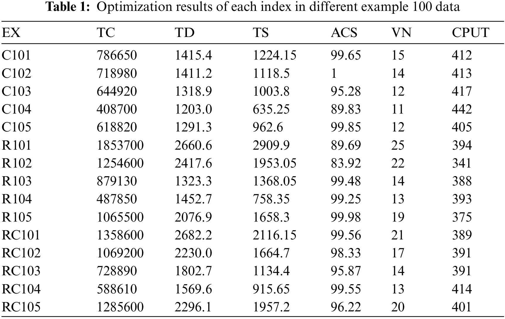
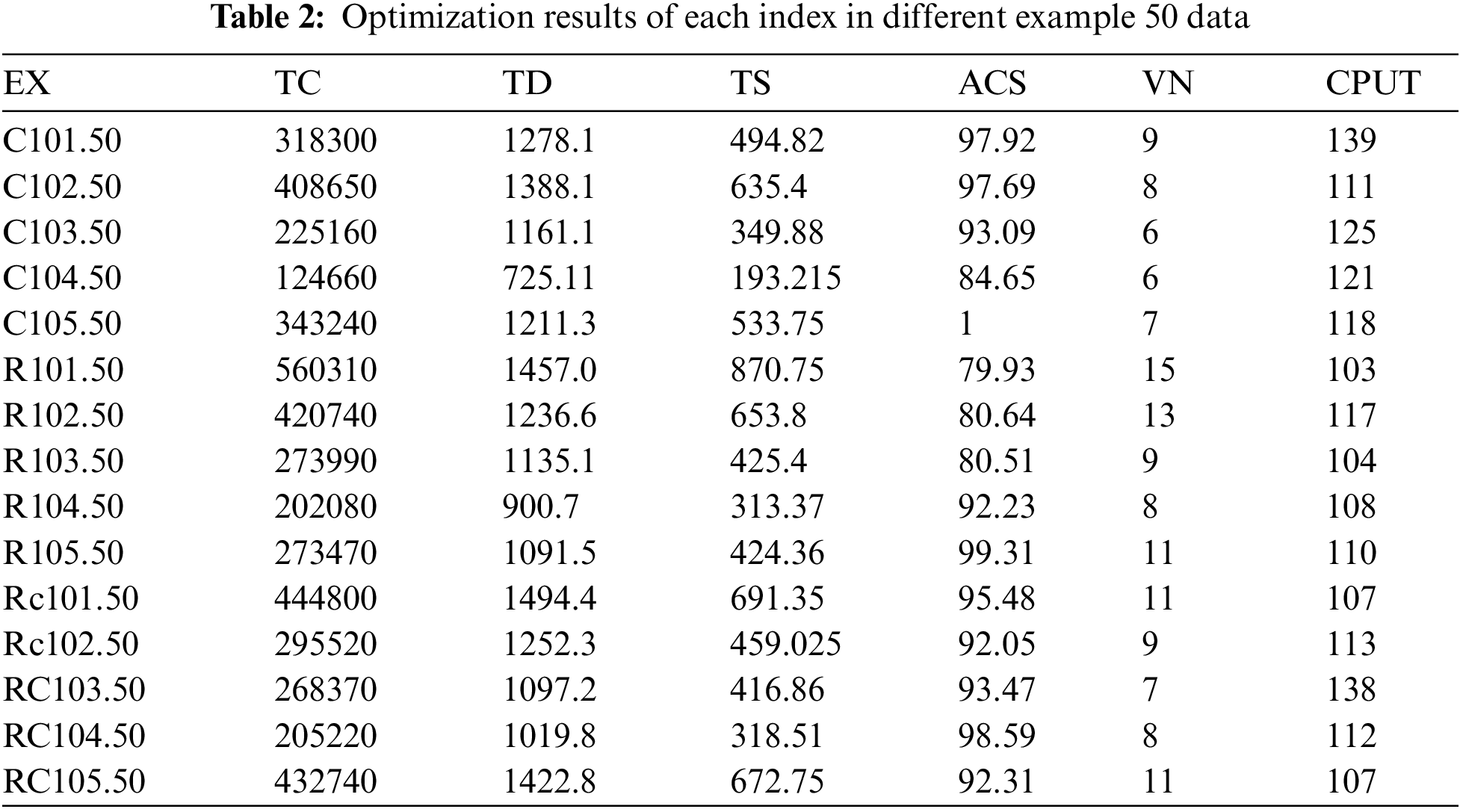
(1)   The maximum running time of the 100 data program is 442 s, and the maximum running time of the 50 data program is 139 s, indicating that the algorithm in this paper can effectively solve different calculation examples in a short time.

(2)   Class C has the lowest total distribution cost, the shortest vehicle driving distance, the lowest carbon tax cost, the least number of vehicles used, but the longest running time. The reason is that the customer distribution of class C calculation example is relatively concentrated, and the distance between each point is short, but the time window and service time are long. Therefore, all the indexes related to distance are small and the running time is long.

(3)   Compared with the C example, the total distribution cost, distribution distance and carbon tax cost of the R and RC examples are larger, and the number of vehicles used is larger. The reason is that the customers of the R and RC examples are randomly distributed, and the distance between each customer is longer, so the items related to distance are larger when completing the delivery. However, the customer time window and service time are short, so the running time is shorter than class C.

(4)   The results of 100 samples and 50 samples selected from all kinds of calculation examples are basically consistent, indicating the correctness of calculation examples.

In this paper, the path planning diagrams of the data of 100 samples and 50 samples are selected for analysis, namely, C101.100, R103.50, RC101.100, and RC103.50. As shown in the following Fig. 1, the distribution path of class C is relatively regular due to the centralized distribution of customers at each point, while the distribution path of class R and RC is not obvious due to the random distribution of customers.

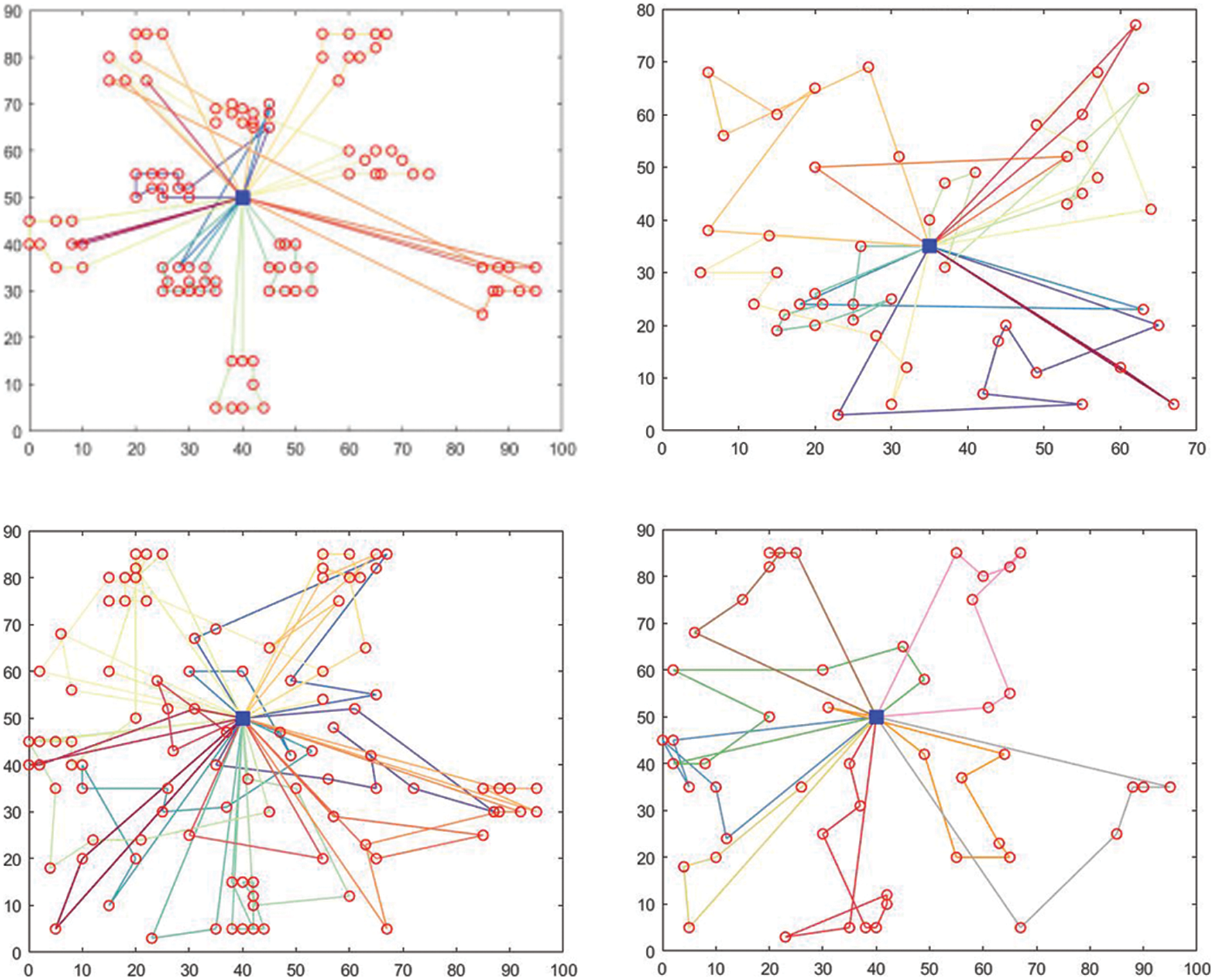
Figure 1: Vehicle routing diagram of C101.100, R103.50, RC101.100, and RC103.50

5.2.2 Optimization Results of Practical Examples

Combined with the model established in this paper and the design algorithm, taking Y cold chain logistics distribution enterprise in Pudong New Area of Shanghai as an example to verify. Mainly based on the 40 customers around the enterprise for distribution, the location, demand, service time window and other information of each customer are shown in Tab. 3. Assume that the vehicle starts from the distribution center and travels at a uniform speed. The vehicle parameters are as follows: S=200 yuan/t,α1=0.02,α2=0.03, β1=15 yuan/h,β2=20 yuan/h, c1=7.25 yuan/L,ω=2.63 kg/L, ρ0=0.165 L/km, ρ∗=0.377 L/km, C0=200 yuan/car:

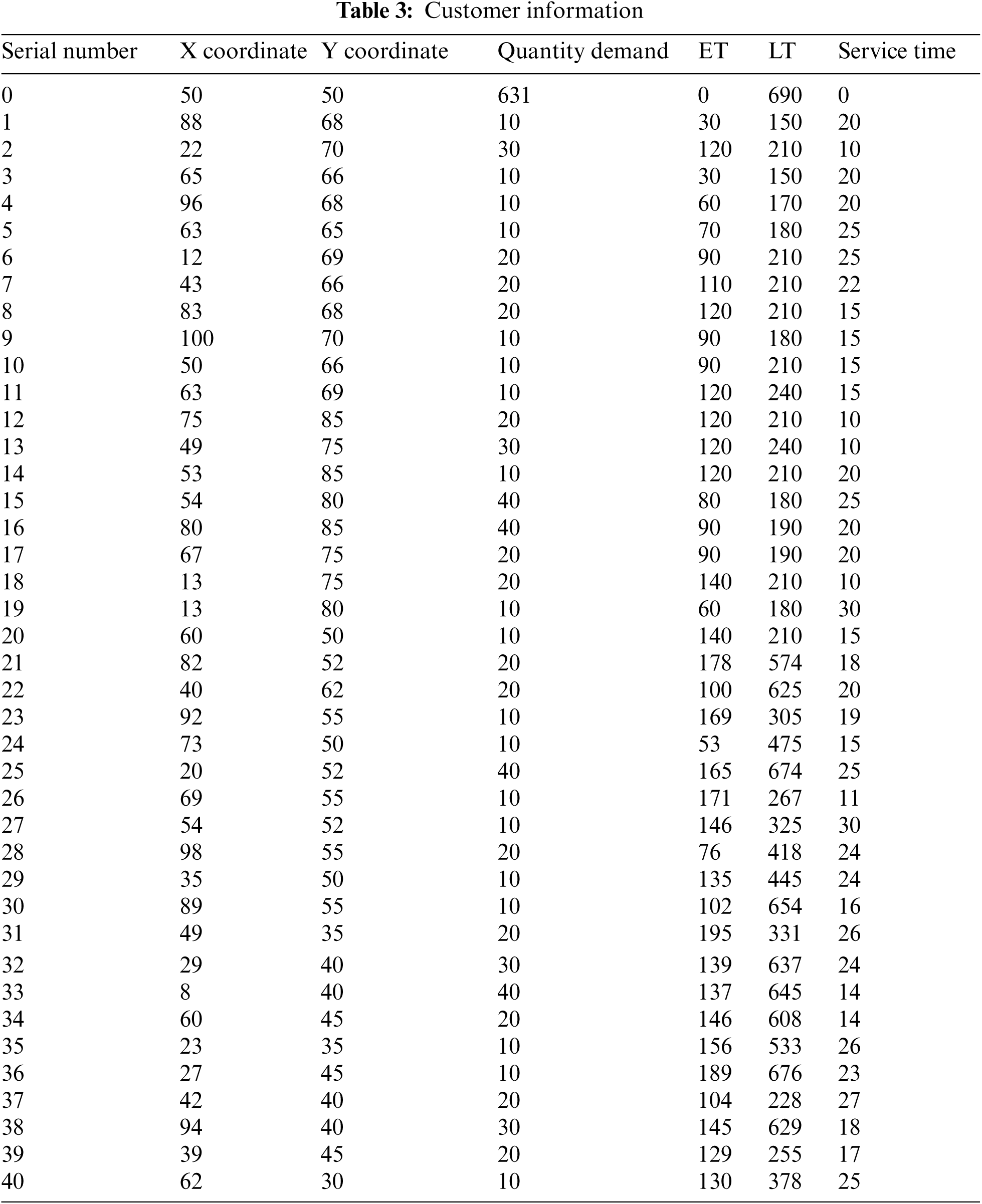
After simulating the target model through MATLAB based on the improved ant colony algorithm, the simulation results of various indicators based on Y enterprise are shown in Tab. 4, the vehicle routing is shown in Fig. 2.

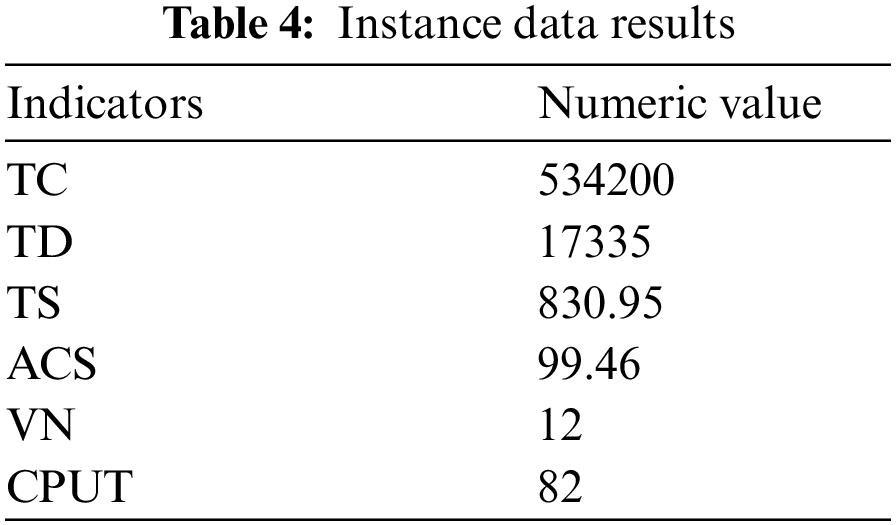
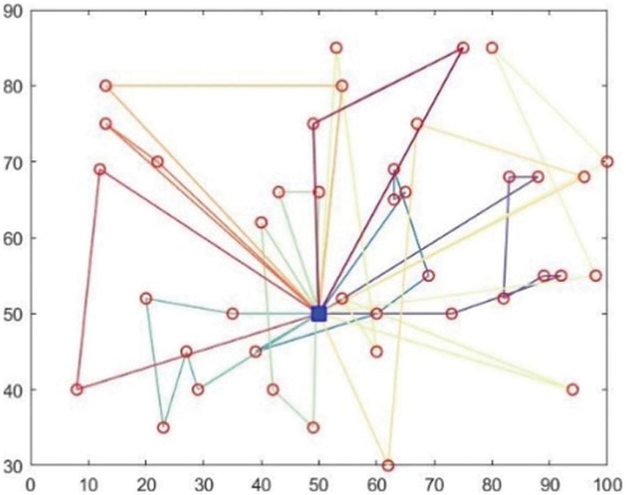
Figure 2: Vehicle routing diagram of example data

It can be seen from the obtained data that the analysis of the case is basically normal, the satisfaction index and other indicators are within the normal range, and the distribution path graph is in line with the normal VRP model operation results.

5.3 Algorithm Comparison Test

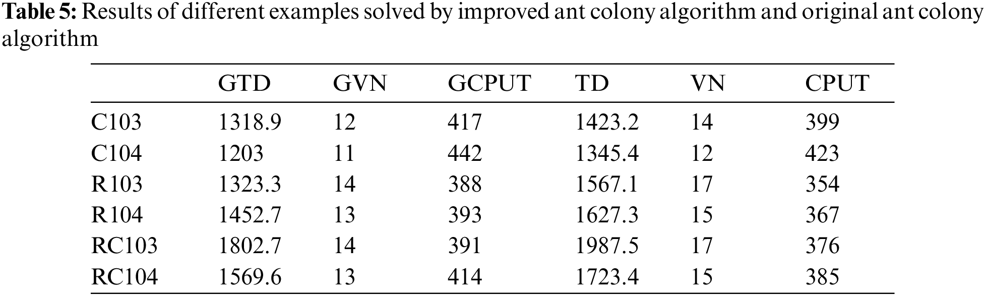
The improved ant colony algorithm and the model considering satisfaction were compared with the original ant colony algorithm and the model not considering satisfaction temporarily, and the advantages of the improved algorithm were observed by comparing the simulation results before and after.

The proposed algorithm was compared with the original ant colony algorithm, and 6 examples of C103, C104, R104, R104, RC103 and RC104 were randomly selected for testing. The parameters will be set as follows: Q=200, max iter=200, m=50, ET/LT extracted from the data of calculation examples. The results are shown in the following Tab. 5.

The model without considering the requirement of satisfaction was simulated, and three data from various calculation examples were selected for analysis, namely, C101.100, C102.100, C103.100, R101.100 and RC101.100. The simulation results are shown in Tab. 6. The vehicle routing diagram is shown in Fig. 3.

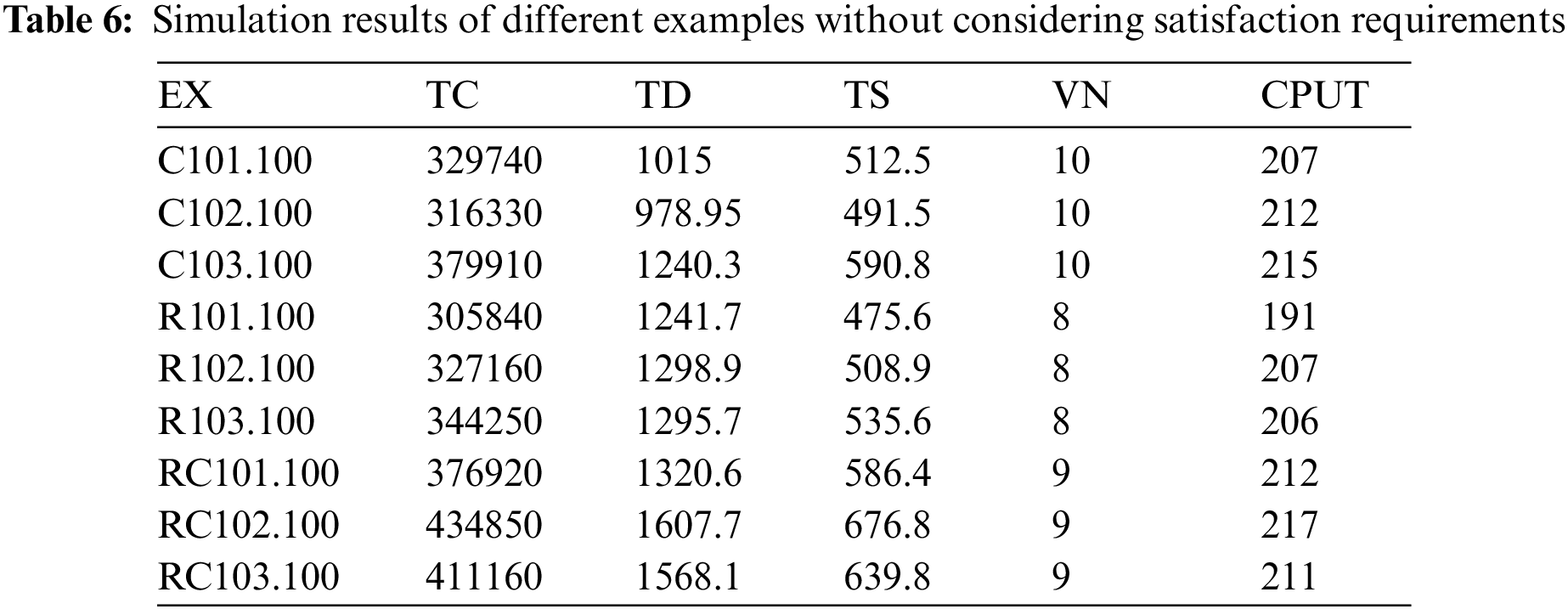
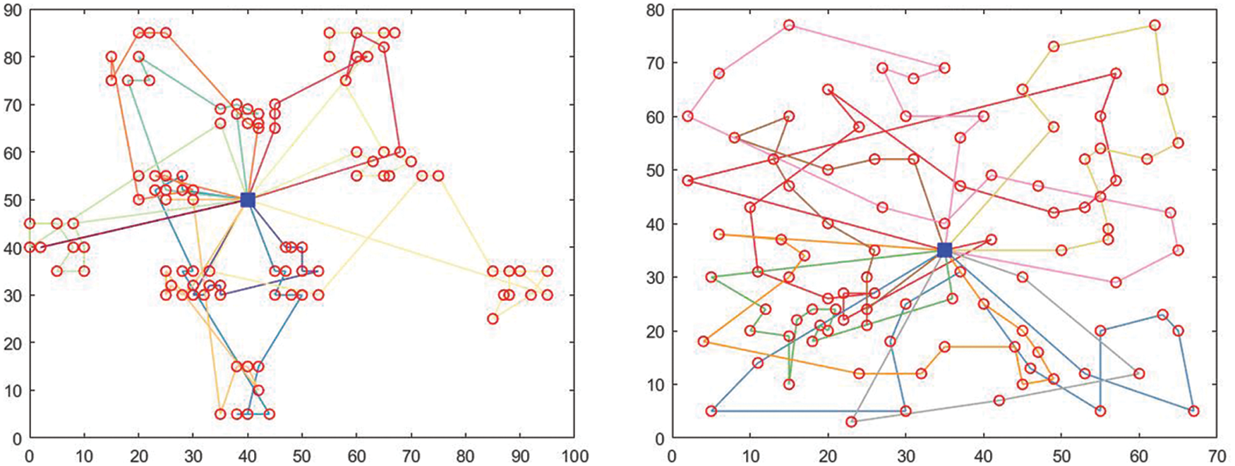
Figure 3: Vehicle routing diagram of C103.100 and R103.100

As can be seen from Tab. 6 and Fig. 3:

(1)   The improved ant colony algorithm is better than the original ant colony algorithm for the six groups of experimental results. For example, the TD of the improved total distribution distance is 1318.9, which is smaller than the original TD1423.2. For the same calculation example and the same data, the number of original vehicles is more than the number of vehicles after the improved algorithm. And the overall running time is longer than the improved ant colony algorithm, so the effectiveness of the improved algorithm is verified on the whole.

(2)   When the objective function does not consider satisfaction, the operation results of all kinds of calculation examples are better than that of satisfaction. For example, the total distribution cost TC of 100 data points of all kinds of calculation examples in the non-objective function of satisfaction is nearly 50% less than that of 100 data points of all kinds of calculation examples in this model, the total distribution path is nearly 34% less, and the overall carbon tax cost is 55% less. And the number of vehicles used has been greatly reduced. The overall running results are in line with the actual situation. When the objective function constraints are reduced, the model optimization does not need to consider too many restrictions, so the running results are better. It shows that the overall distribution efficiency is higher and the cost is lower without considering the customer satisfaction at the completion of the distribution state.

(3)   As shown in Fig. 3, when satisfaction is not an objective function, the overall running roadmap still conforms to the distribution of various calculation examples, indicating the correctness and rationality of the algorithm. At the same time, when satisfaction is not a part of the objective function, although the overall running route still conforms to the distribution of calculation examples, there is no need to consider too many limiting factors in algorithm simulation due to the reduction of objective function optimization objectives, and the most convenient and fast distribution route can be selected from the feasible distribution scheme to complete all the distribution tasks. Therefore, all indicators in the overall running results are smaller than the original target model, which conforms to the theoretical logic, indicating that the calculation example is correct.

6  Conclusion

This paper proposed an optimization model of low carbon fresh cold chain logistics distribution path considering customer satisfaction, and combined with time window constraints, load limit and delivery requirements to optimize the distribution model, at the same time, transportation cost, penalty cost, overloading cost, carbon tax cost and customer satisfaction were considered as the components of the objective function, and the thought of cost efficiency was taken into account, so as to establish a distribution model based on the ratio of minimum total cost to maximum satisfaction as the objective function. After that, the improved A* algorithm and ant colony algorithm were combined to conduct simulation analysis on the objective function. The simulation data came from VRP database and real example data. Then through MATLAB software simulation analysis, and get simulation data results and roadmap. Simulation results show that:

(1)   The improved ant colony algorithm can effectively reduce the total distribution cost, reduce carbon emissions and reduce the number of vehicles used;

(2)   The overall distribution cost of the improved ant colony algorithm increases compared with the original algorithm due to the consideration of carbon tax;

(3)   The overall optimization model conforms to VRP optimization results, indicating the correctness of the model constructed in this paper.

7  Discussion

This paper focuses on the optimization of low-carbon fresh cold chain transportation model based on customer satisfaction. However, because the whole model is based on the constraint conditions of assumed distribution requirements and distribution results, there are still many different solutions for different distribution requirements. Therefore, in the future research, in-depth research can be conducted on the following types:

(1)   The problem studied in this paper is that fresh products can be applied to logistics operations at the same temperature environment, but there are various types of fresh products distributed in real life, and the appropriate temperature of many products is not the same. Therefore, the optimization research of fresh cold chain logistics distribution with multi-temperature coordination can be carried out in the future.

(2)   For the convenience of calculation, the speed of vehicle transportation is set as a constant value in this paper. But in the actual situation, the distribution environment is limited by the distribution time, distribution environment, distribution location, etc. Generally speaking, the vehicle distribution speed is dynamic change. Therefore, in future studies, the real-time speed of cold chain distribution vehicles under time-varying road network conditions can be calculated.

(3)   This paper assumes that the vehicle does not need to return to the distribution point after completing the task of reaching the distribution point from the distribution center. Therefore, the subsequent operation of vehicles will not be included in the consideration center of the whole system. However, based on the actual distribution situation, after completing the distribution task, most vehicles need to return to the original distribution center, and the route planning scheme required for the return trip is missing. Therefore, the future research direction can be based on the overall planning of the route after the vehicle completes the delivery task and returns.

Funding Statement: This research was funded by the China education ministry humanities and social science research youth fund project (No. 18YJCZH192), the Applied Undergraduate Pilot Project for Logistics Management of Shanghai Ocean University (No. B1–5002–18–0000), the social science project in Hunan province (No. 16YBA316).

Conflicts of Interest: The authors declare that they have no conflicts of interest to report regarding the present study.

Reference

 1.  OECD iLibrary, 2021. [online]. Available: https://www.oecd-ilibrary.org/energy/data/iea-co2-emissions-from-fuel-combustion-statistics_co2-data-en. [Google Scholar]

 2.  Y. H. Hsiao, M. C. Chen, K. Y. Lu and C. L. Chin, “Last-mile distribution planning for fruit-and-vegetable cold chains,” The International Journal of Logistics Management, vol. 29, no. 3, pp. 862–886, 2018. [Google Scholar]

 3.  S. Erdoğan and E. Miller-Hooks, “A green vehicle routing problem,” Transportation Research Part E Logistics & Transportation Review, vol. 48, no. 1, pp. 100–114, 2012. [Google Scholar]

 4.  J. Wang, S. Yao, J. Sheng and H. Yang, “Minimizing total carbon emissions in an integrated machine scheduling and vehicle routing problem,” Journal of Cleaner Production, vol. 229, pp. 1004–1017, 2019. [Google Scholar]

 5.  G. Poonthalir and R. Nadarajan, “A fuel efficient green vehicle routing problem with varying speed constraint (F-GVRP),” Expert Systems with Applications, vol. 100, pp. 131–144, 2018. [Google Scholar]

 6.  D. Wu and C. Wu, “TDGVRPSTW of fresh agricultural products distribution: Considering both economic cost and environmental cost,” Applied Sciences, vol. 11, no. 22, pp. 1–24, 2021. [Google Scholar]

 7.  M. M. Solomon, “Algorithms for the vehicle routing and scheduling problems with time window constraints,” Operations Research, vol. 35, no. 2, pp. 254–265, 1987. [Google Scholar]

 8.  M. Gendreau, F. Guertin, J. Potvin and E. Taillard, “Parallel tabu search for real-time vehicle routing and dispatching,” Transportation Science, vol. 33, no. 4, pp. 381–390, 1999. [Google Scholar]

 9.  T. Ou, C. Cheng, C. H. Lai and H. Fu, “A Coordination-based algorithm for dedicated destination vehicle routing in B2B e-commerce,” Computer Systems Science and Engineering, vol. 40, no. 3, pp. 895–911, 2022. [Google Scholar]

10. M. M. Altaf, A. S. Roshdy and H. S. Al Sagri, “Deep reinforcement learning model for blood bank vehicle routing multi-objective optimization,” Computers, Materials & Continua, vol. 70, no. 2, pp. 3955–3967, 2022. [Google Scholar]

11. B. Zhao, H. Gui, H. Li and J. Xue, “Cold chain logistics path optimization via improved multi-objective ant colony algorithm,” IEEE Access, vol. 8, pp. 142977–142995, 2020. [Google Scholar]

12. G. Qin, F. Tao and L. Li, “A vehicle routing optimization problem for cold chain logistics considering customer satisfaction and carbon emissions,” International Journal of Environmental Research & Public Health, vol. 16, no. 4, pp. 576–593, 2019. [Google Scholar]

13. F. E. Zulvia, R. J. Kuo and D. Y. Nugroho, “A many-objective gradient evolution algorithm for solving a green vehicle routing problem with time windows and time dependency for perishable products,” Journal of Cleaner Production, vol. 242, pp. 118428.1–118428.14, 2020. [Google Scholar]

14. D. Wu, Y. Liu, K. Zhou, K. Li and J. Li, “A multi-objective particle swarm optimization algorithm based on human social behavior for environmental economics dispatch problems,” Environmental Engineering and Management Journal, vol. 18, no. 7, pp. 1599–1607, 2019. [Google Scholar]

15. X. Zhang, W. Zhang, W. Sun, X. Sun and S. K. Jha, “A robust 3-D medical watermarking based on wavelet transform for data protection,” Computer Systems Science & Engineering, vol. 41, no. 3, pp. 1043–1056, 2022. [Google Scholar]

16. Y. Xue, Y. Tang, X. Xu, J. Liang and F. Neri, “Multi-objective feature selection with missing data in classification,” IEEE Transactions on Emerging Topics in Computational Intelligence, vol. PP, no. 99, pp. 1–10, 2021. [Google Scholar]

17. Y. Xue, H. Zhu, J. Liang and A. Sowik, “Adaptive crossover operator based multi-objective binary genetic algorithm for feature selection in classification,” Knowledge-Based Systems, vol. 227, no. 5, pp. 1–9, 2021. [Google Scholar]

18. D. Q. Wu, M. Dong, H. Y. Li and F. Li, “Vehicle routing problem with time windows using multiobjective co-evolutionary approach,” International Journal of Simulation Model, vol. 15, no. 4, pp. 742–753, 2016. [Google Scholar]

19. X. R. Zhang, X. Sun, X. M. Sun, W. Sun and S. K. Jha, “Robust reversible audio watermarking scheme for telemedicine and privacy protection,” Computers, Materials & Continua, vol. 71, no. 2, pp. 3035–3050, 2022. [Google Scholar]

20. T. Vidal, G. Laporte and P. Matl, “A concise guide to existing and emerging vehicle routing problem variants,” European Journal of Operational Research, vol. 286, no. 2, pp. 401–416, 2020. [Google Scholar]

21. X. P. Wang, K. Zhang and H. U. Xiang-Pei, “Research of vehicle routing problem based on fuzzy time windows,” Journal of Industrial Engineering/Engineering Management, vol. 25, no. 3, pp. 148–154, 2011. [Google Scholar]

22. L. Lin, S. Liu and J. Tang, “Improved ant colony algorithm for solving vehicle routing problem with time windows,” Control and Decision, vol. 25, no. 9, pp. 1379–1383, 2010. [Google Scholar]

23. R. D. Ottmar, “Wildland fire emissions, carbon, and climate: Modeling fuel consumption,” Forest Ecology and Management, vol. 317, pp. 41–50, 2014. [Google Scholar]

24. E. Demir, T. Bekta and G. Laporte, “A comparative analysis of several vehicle emission models for road freight transportation,” Transportation Research Part D Transport and Environment, vol. 16, no. 5, pp. 347–357, 2011. [Google Scholar]

25. Y. Xiao, Q. Zhao, I. Kaku and Y. Xu, “Development of a fuel consumption optimization model for the capacitated vehicle routing problem,” Computers & Operations Research, vol. 39, no. 7, pp. 1419–1431, 2012. [Google Scholar]

26. Y. Xiao and A. Konak, “The heterogeneous green vehicle routing and scheduling problem with time-varying traffic congestion,” Transportation Research Part E, vol. 88, pp. 146–166, 2016 [Google Scholar]

This work is licensed under a Creative Commons Attribution 4.0 International License, which permits unrestricted use, distribution, and reproduction in any medium, provided the original work is properly cited.