Computers, Materials & Continua DOI:10.32604/cmc.2022.028416
Article

Incremental Learning Model for Load Forecasting without Training Sample

Charnon Chupong and Boonyang Plangklang*

Faculty of Engineering, Rajamangala University of Technology Thanyaburi, Pathum Thani, 12110, Thailand
*Corresponding Author: Boonyang Plangklang. Email: boonyang.p@en.rmutt.ac.th
Received: 09 February 2022; Accepted: 14 March 2022

Abstract: This article presents hourly load forecasting by using an incremental learning model called Online Sequential Extreme Learning Machine (OS-ELM), which can learn and adapt automatically according to new arrival input. However, the use of OS-ELM requires a sufficient amount of initial training sample data, which makes OS-ELM inoperable if sufficiently accurate sample data cannot be obtained. To solve this problem, a synthesis of the initial training sample is proposed. The synthesis of the initial sample is achieved by taking the first data received at the start of working and adding random noises to that data to create new and sufficient samples. Then the synthesis samples are used to initial train the OS-ELM. This proposed method is compared with Fully Online Extreme Learning Machine (FOS-ELM), which is an incremental learning model that also does not require the initial training samples. Both the proposed method and FOS-ELM are used for hourly load forecasting from the Hourly Energy Consumption dataset. Experiments have shown that the proposed method with a wide range of noise levels, can forecast hourly load more accurately than the FOS-ELM.

Keywords: Incremental learning; load forecasting; Synthesis data; OS-ELM

1  Introduction

Global photovoltaic system deployments from 2017 to 2020 increased from 384.45 to 707.50 GW, representing an approximately 84% increase in three years [1]. By 2020, global electric vehicle registrations increased by 41%, bringing the total number of electric vehicles to about 10 million [2]. By the end of 2020, 5 GW of grid-sized energy storage systems has been installed globally, a 50% increase from mid-2019 and a steady increase [3]. All of the above events have resulted in a dramatic change in electricity usage patterns from the past. Therefore, the models used for electrical load forecasting need to be constantly updated according to the changes in the patterns of electricity consumption. But in general, those conventional models cannot learn from newly received data to adapt themselves during operation. Improving the models require new and sufficient data to re-train the model from scratch, which time consuming and inconvenient.

To solve this problem, researchers have developed a model that can learn from newly received data without forgetting what was previously learned, called incremental learning. The examples of incremental learning include Incremental Support Vector Machine (ISVM) [4], Online Random Forecast (ORF) [5], Incremental Learning Vector Quantization (ILVQ) [6], Learn++ [7], Stochastic Gradient Descent (SGD) [8], and Online Sequential Extreme Learning Machine (OS-ELM) [9]. In this article, OS-ELM was chosen because it is a fast-learning model suitable for short-term load forecasting and easy to implement in hardware with low computational power. OS-ELM is a single hidden layer feed-forward neural network model where the weights in the input layer are randomly generated and retained over time, while hidden layer weights are computed based on a recursive least square method. This structure allows OS-ELM to function similarly to conventional neural networks but learning speed is more quickly. The OS-ELM requires initial samples for initial training, the amount of this initial sample must be more or equal to the number of nodes in the OS-ELM hidden layer. Usually, the number of nodes in this hidden layer affects forecast accuracy, implying that the amount of initial training data also affects the forecast accuracy.

In the implementation of OS-ELM, there are cases where a sufficient initial training sample cannot be obtained, such as a new building or building that never records the electricity usage data. Such a problem may be solved by the Transfer Learning technique [10], where data from other similar tasks is used as the source for initial training. But users cannot be sure whether the source data is similar to the real data or not. The researchers later proposed improvements to the OS-ELM model so that it can be used without an initial training sample called Fully Online Sequential Extreme Learning Machine (FOSELM) [11].

In the image classification and object detection research field, there is a method to solve the insufficient training samples problem by creating augmented samples from real samples [12]. For example in [13], the authors use the Mosaic data augmentation method to create more training samples. But in the load forecasting research field, there are few studies on using the augmented sample to train the forecasting models.

To the convenient use of OS-ELM especially in the case of new buildings or buildings without historical data of energy usage, this article proposed a method that allows OS-ELM to be used without the need for initial training samples. The proposed method takes a single sample through the synthesis process by adding random noise. The synthesis process makes enough new samples for the initial training of the OS-ELM. The proposed method was compared to the FOSELM in short-term load forecasting using a dataset called Hourly Energy Consumption [14]. The dataset was based on the hourly electricity consumption of cities in the Eastern United States from nine utility companies. The rest of this article contains related research in part 2, the proposed method is presented in part 3, the experiment and results in part 4, analysis of the experimental results in part 5, and conclusion in part 6.

2  Related Research

2.1 Load Forecasting

Load forecasting is an integral part of the smart grid. Numerous studies have been conducted on load forecasting [15], load forecasting is divided into four forecasting periods.

1.    Very short-term load forecasting is a forecast up to 1 h in advance where the forecast result is often used to control the power system quality.

2.    Short-term load forecasting is a forecast one hour but not more than a week in advance. The forecast result is often used to balance the supply and demand use of electricity.

3.    Medium-term load forecasting is a forecast one month but not more than 1 year in advance. The forecast result is often used in planning the fuel supply in the electricity generation.

4.    Long-term load forecasting is a forecast more than one year in advance. The forecasting result is often used in investment planning in power plants or power system infrastructure.

There are two main models used for load forecasting that are commonly found in research.

1.    Auto Regressive Integrated Moving Average (ARIMA) is popular for time series data analysis. ARIMA consists of:

       a)  The Autoregressive (AR) part describes the linear regression between current data and past data, and

       b)  The Moving Average (MA) part describes linear regression between current data and past forecast errors caused by white noise in the data.

          AR and MA are only applicable for stationary data. To improve AR and MA model to be applicable with non-stationary data “Integrated” part has been added and called ARIMA.

2.    Artificial Neural Network (ANN) in time series forecasting the ANN model differs from the ARIMA model in that it can use non-linear activation functions and hidden layer structures. That allows the ANN can predict the non-linear relationship between input and output better than ARIMA models [16].

2.2 Incremental Learning

Modeling for load forecasting requires historical sample data to calculate parameters in the model. In ANN, various machine learning techniques are used to calculate ANN’s parameters, this process is called “training”. The sample data used for training must be sufficiently large and should have a pattern similar to the data that the model must forecast. The training is done once at the beginning of the operation, known as batch learning. But at present, the pattern of electricity load has changed all the time due to photovoltaic systems [17–19] electric vehicles [20,21], and energy storage systems [22,23]. Therefore models created by batch training method require constantly re-training the model from scratch to be able to forecast accurately. The re-training in such cases creates inconvenience in practice. Therefore, researchers have introduced a model that can learn from new incoming data and still remember the past data, known as online learning or incremental learning. There are some examples of incremental learning such as.

•   Incremental Support Vector Machine (ISVM) [4] incremental version of Support Vector Machine (SVM) working by storage some data as “candidate vector”. This candidate vector may be promoted as “support vector” according to newly receive data during operation.

•   Online Random Forest (ORF) [5] works like Random Forecast, but the number of trees (the number of sub-models) increases if the new data received changes from the past data.

•   Incremental Learning Vector Quantization (ILVQ) [6] a Learning Vector Quantization (LVQ) that can be expanded by increasing the number of prototypes in the model when the new data received changes from the past data.

•   Learn++ [7] uses the same principle as the ensemble model like AdaBoost [24]. Sub-model is added and trained with new data that is randomly selected from past data. Data samples with high forecasting errors are more likely to be selected, therefore Learn++ can adjust according to changes in data.

•   Stochastic Gradient Descent (SGD) [8] is an optimization method for adjusting the model’s parameters without needing to use the entire batch of data at once. The model’s parameter can be adjusted according to the change of newly received data.

•   Online Sequential Extreme Learning Machine (OS-ELM) [9] is an incremental model that is characterized by learning speed and low computation cost allowing it to run on the machine with low computational power. The details of the OS-ELM are presented in the next sections.

2.3 Extreme Learning Machine (ELM)

ELM structure is like a single hidden layer feed-forward neural network (SLFN) model. The ELM was first introduced by Guang et al. in 2004 [25]. The most outstanding feature of ELM is its extremely high learning speed since ELM does not use an iterative method such as gradient descent to calculate the parameters but uses the normal equation instead. The structure of the ELM is shown in Fig. 1. The bias and weight values that are connected between the input and the hidden layer are randomly generated and remain constant. While the weight between the hidden layer and the output layer is calculated by the normal equation as follows.

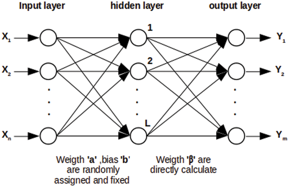
Figure 1: ELM Structure

If the dataset has N samples called (xj,yj) where xj∈Rn and yj∈Rm numbers of nodes in the hidden layer equal to L relationship between xj and yj can be defined as follows.

yj=∑i=1Lβig(aixj+bi),j=1,2,….N(1)

where βi∈Rm are weights in the hidden layer, g(…):R→R is an activation function in the hidden layer, ai∈Rn are weights in the input layer, and bi∈R are bias in input layer, Eq. (1) can be re-write in more simple form as follows:

Y=Hβ(2)

where

Matrix H is called “Hidden layer output matrix” ai and bi are constant from random generated, causing H is also constant, therefore training ELM is calculating β as in Eq. (2). If the number of data or dimensions is not too large, the normal equation can be directly calculated more quickly as compared to the Gradient Descent method. β can be calculated as follows:

β=(HTH)−1HTY(3)

or

β=K−1HTYwhereK=HTH(4)

Although ELM uses random weights and bias values in the input layer, many studies have shown that ELM has good performance as other learning algorithms [26,27]. The ELM model may encounter problems with numerical stability since sometimes inversion of the matrix HTH is not possible, the Singular Value Decomposition (SVD) method has been proposed [28] to find the inverse of HTH.

2.4 Regularization Extreme Learning Machine (Re-ELM)

Numerical stability problems of the ELM model can be solved by adding the regularization factor [29] for calculating matrix K as shown in Eq. (5) which lowers the cost of computational than SVD.

K=HTH+λI(5)

where λ is a very small value called the regularization factor and I is the identity matrix.

2.5 Online Sequential Extreme Learning Machine (OS-ELM)

The ELM model is a batch learning method, where it uses all available data to train the model and make the model work. While the model is running, it cannot learn more from the new incoming data. Therefore, a research paper proposed an improvement of the ELM model to be able to perform incremental learning called the Online Sequential Extreme Learning Machine (OS-ELM) [9] using the recursive principle of Eq. (4). At the beginning of work, the OS-ELM will calculate β0=K0−1H0TY0 where K0=H0TH0 which subscript 0 mean round 0 of work or initial of work. When OS-ELM receives new sample(s) data causing the value of matrix H and Y change, therefore β1 can be calculated as follows.

β1=K1−1[H0H1]T[Y0Y1](6)

K1=K0+H1TH1(7)

and

Substitute the K0 value from Eq. (7) into the above equation.

[H0H1]T[Y0Y1]=K1β0−H1TH1β0+H1TY1(8)

Substitute Eq. (8) into Eq. (6).

β1=β0+K1−1H1T(Y1−H1β0) where

K1=K0+H1TH1(9)

Eq. (9) can be arranged in a general recursive form as:

βk+1=βk+Kk+1−1Hk+1T(Yk+1−Hk+1βk)whereKk+1=Kk+Hk+1THk+1(10)

The subscription k means the kth samples and the subscription k+1 means the (k+1)th samples. Each incoming sample does not need to be equal in numbers. In short, the OS-ELM works in two steps as follows.

•   The initial step is like the ELM, the initial samples are used to calculate β0 by Eq. (4). The number of initial samples needs to be more than or equal to the number of nodes in a hidden layer of the model.

•   The incremental learning step uses the newly receives sample to adjust the model parameters as in Eq. (10).

2.6 Regularization Online Sequential Extreme Learning Machine (ReOS-ELM)

Like the ELM, if k is a non-invertible matrix then the OS-ELM has a numerical stability problem that can be solved by adding a regularization factor [30] as shown in Eq. (11).

Kk+1=Kk+Hk+1THk+1+λI(11)

where λ is a very small value called the regularization factor and I is the identity matrix.

2.7 Fully Online Sequential Extreme Learning Machine (FOS-ELM)

The OS-ELM and ReOS-ELM require samples for initial training, but in some situations, we are unable to obtain enough appropriate samples for initial training. Therefore, the FOS-ELM model is presented, which is a model that does not need the initial data for initial training [11] by setting initial parameters β0=0, K0=λI. In other words, the FOS-ELM is initial training by the initial sample (X=0,Y=0).

3  Proposed Method

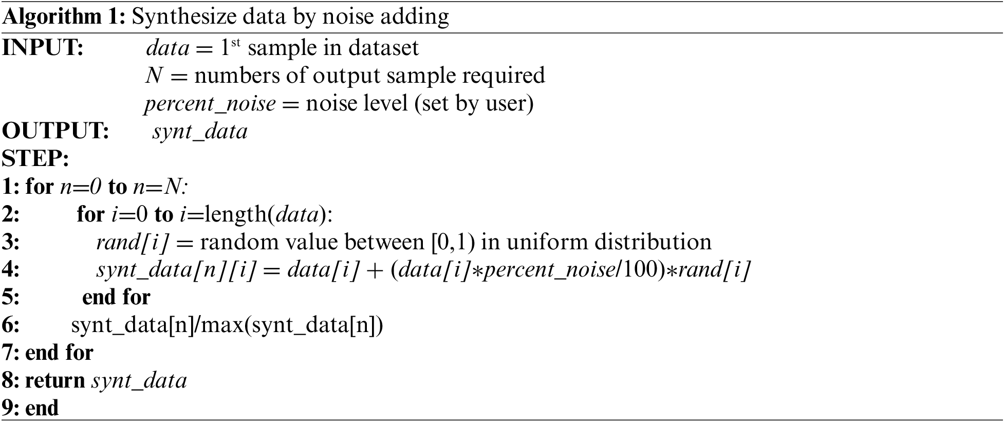
As mentioned above, the implementation of OS-ELM require sufficient and appropriate initial training samples. But in some situations, those samples cannot be obtained. Therefore, in this article, we present a method to solve that problem. The method presented in this article uses a single sample received at the start of working to synthesize sufficiently the initial training data. The data synthesis method is done by adding random noise to all features of the sample to create new samples. The noise is randomly generated according to uniform distribution and the user can adjust the level of noise that to be added to the sample called “percent noise”. This proposed method can be described as a diagram in Fig. 2 and an algorithm 1. Please note that this article uses ReOS-ELM instead of OS-ELM to avoid the numerical stability problem.

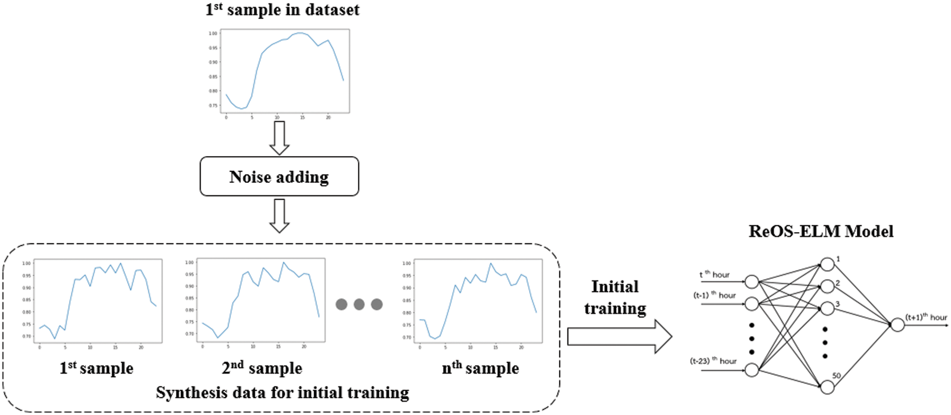
Figure 2: Diagram of the proposed method

To improve forecasting accuracy, ten ReOS-ELM models were combined to form an ensemble model and the mean function is used as an ensemble function. In other words, the forecast values are obtained by averaging the 10 forecast values from all ReOS-ELM models. All 10 models are learning from the same sample both the initial training phase and the incremental learning phase as shown in Fig. 3.

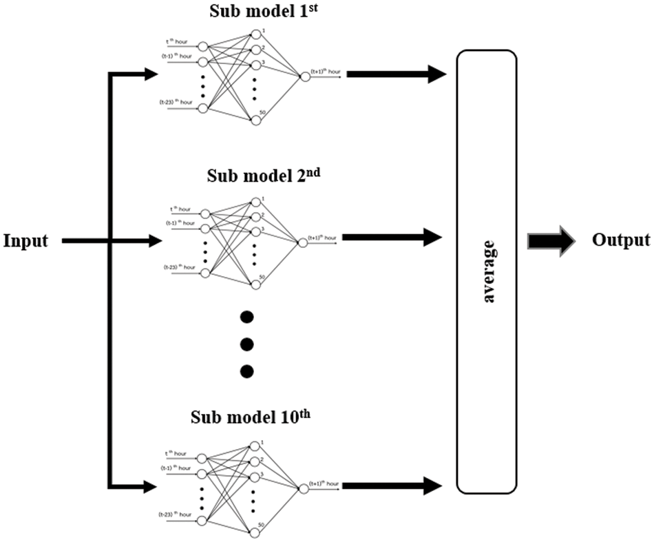
Figure 3: The proposed ensemble model

4  Experiment Results and Discussion

This experiment uses a dataset from https://www.kaggle.com named “Hourly Energy Consumption” [14], which is the hourly electricity usage (hourly load profile) of cities in the eastern United States that gathered from nine utility companies. In the experiment, data are divided into two parts: (1) target is the 1-hour load each and (2) input is the 24-h load before the target as shown in Fig. 4. Inputs are fed to the model so that the model forecasts the next hour's load. The forecast values obtained from the model are compared to the target and forecasting errors can be determined. Both the input and the target are used in the model for incremental learning. The model uses an ensemble model as shown in Fig. 3, where the sub-model is ReOS-ELM with 24 nodes in input layers, 50 nodes in hidden layers, and 1 node in the output layer. The hidden layer uses Sigmoid as the activation function.

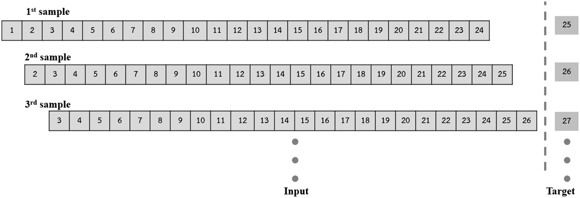
Figure 4: Dataset is divided into Input and Target

The experiment in this article uses two incremental learning models: (1) the FOS-ELM model is the baseline for comparison, and (2) the ReOS-ELM model trained with 50 synthesized samples by the method presented in Section 3. In addition, various percent noises for synthesizing the sample are also tested to determine the appropriate values. The experimental flowchart is shown in Fig. 5, using the first 72 h of data in the dataset to study the early phase of the forecasting operation.

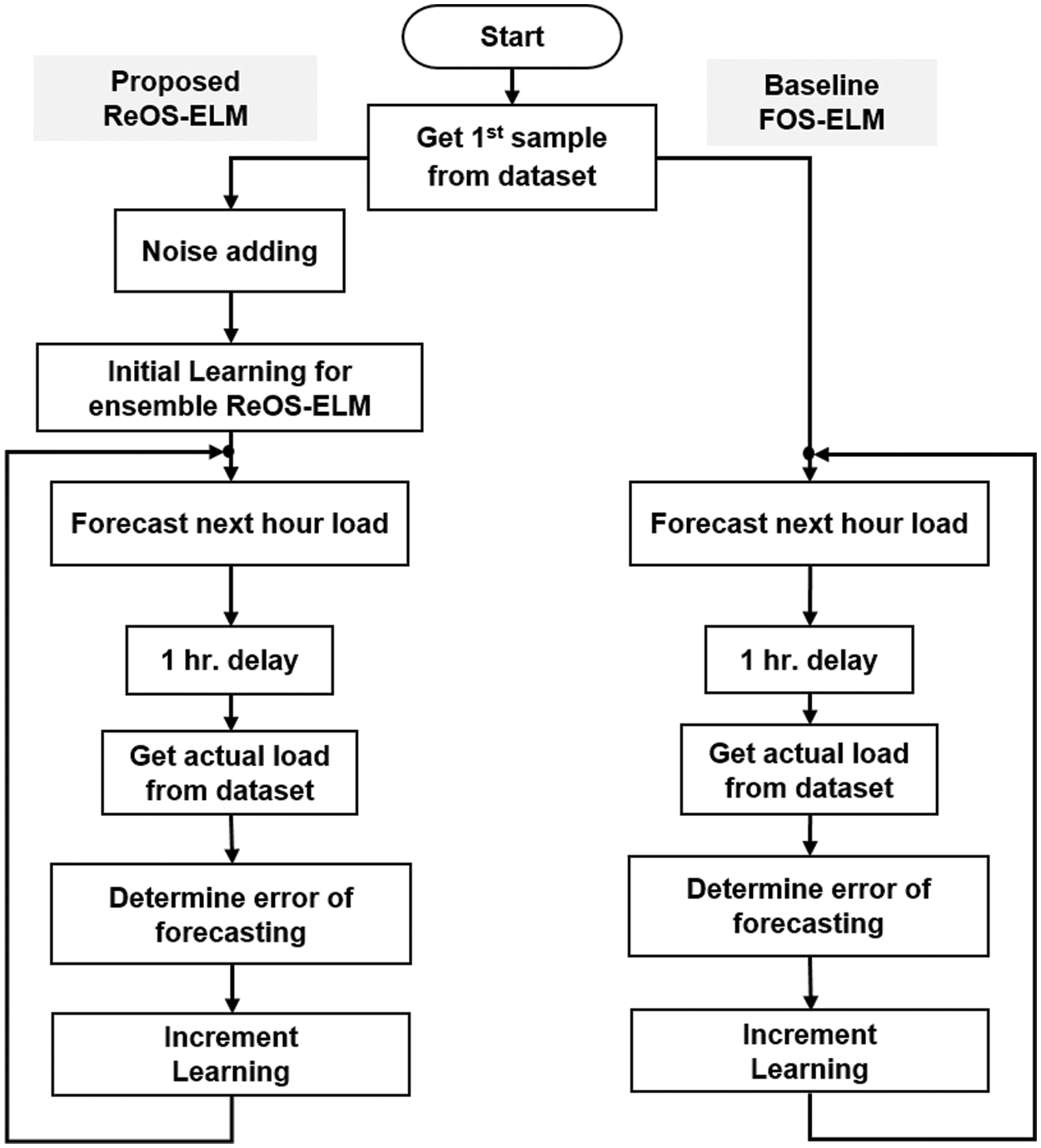
Figure 5: Flow chart of the experiment

The performance metrics used to compare the accuracy of the forecasting is Mean Absolute Percentage Error (MAPE) and Mean Absolute Error (MAE). The experimental results are shown in Tab. 1.

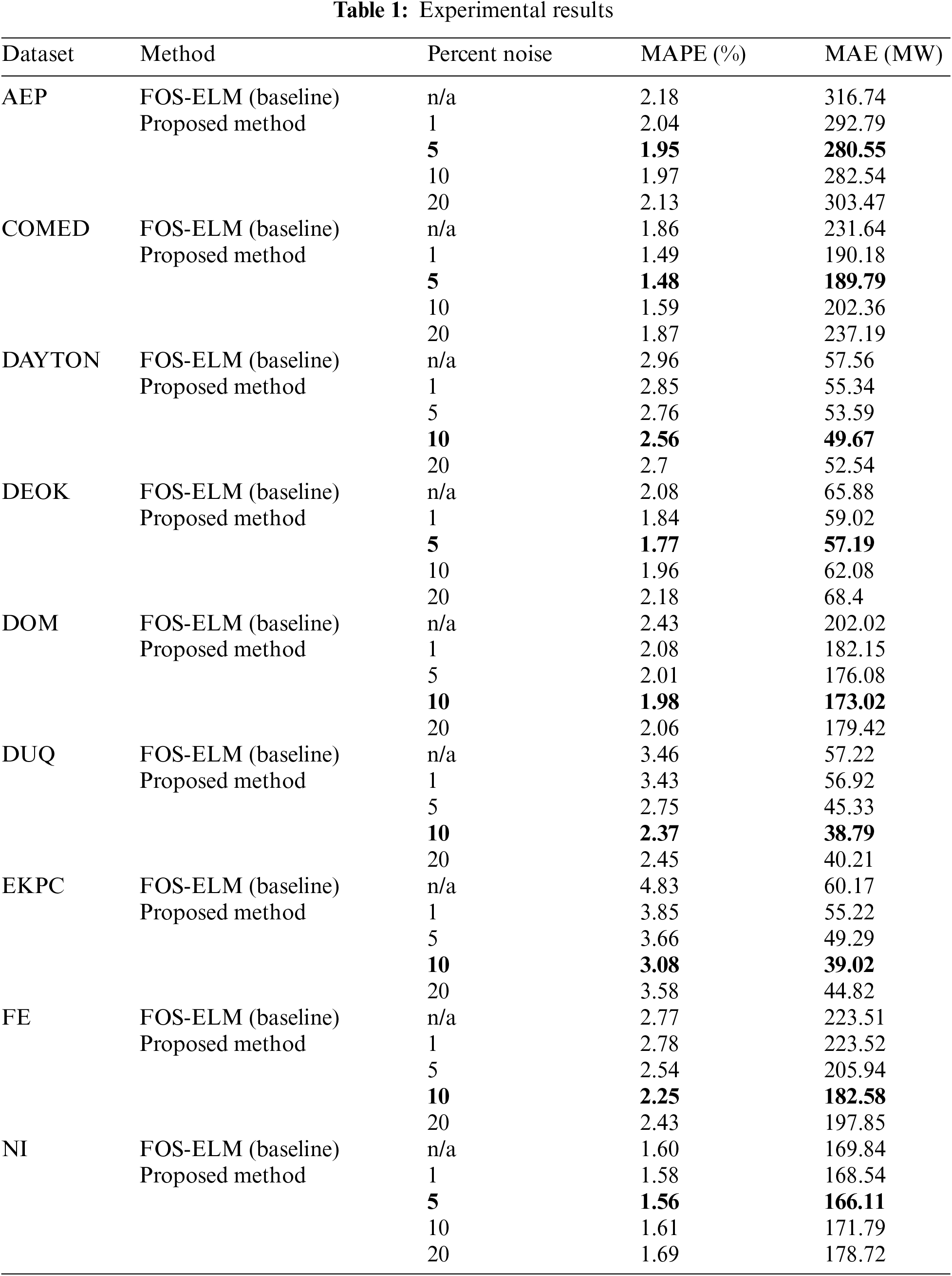
From the results in Tab. 1, it was found that using the ReOS-ELM trained with samples synthesized by the proposed method can achieve lower forecasting error than the FOS-ELM. This is because FOS-ELM is like using a single sample for the initial training, resulting in the model facing the over-fit problem. While the ReOS-ELM model uses synthesized samples with sufficient numbers for the initial training, so the over-fit problems can be avoided.

From the experiment, it was found that the appropriate percent noise is flexible. That is to say, the forecasting error of the ReOS-ELM still lower than the FOS-ELM regardless of the percent noise value (except in the EKPC and FE dataset, when 1% percent noise is used, forecasting error of the ReOS-ELM is slightly higher than the FOS-ELM).

Different forecasting errors that occur when using different percent noise may be caused by the following reasons. At low percent noise, the synthesized samples for initial training are similar to each other, making the model more prone to over-fit problems. At high percent noise, the synthesized samples for initial training may differ from the real data, this makes the model prone to under-fit problems. The experiment found that approximately 5%–10% noise levels resulted in the lowest forecasting error.

5  Conclusion

The proposed method can allow ReOS-ELM or OS-ELM to run without an example for initial training. By adding noise to a single sample received at the start of the operation to increase the number of samples to be sufficient for initial training. The experiment found that whether using noise levels 1%, 5%, 10%, or 20% the ReOS-ELM can forecast loads more accurately than the FOS-ELM. The noise level for synthesis initial samples that allow the ReOS-ELM model to the most accurate forecasting is about 5%–10%.

Funding Statement: The authors received no specific funding for this study.

Conflicts of Interest: The authors declare that they have no conflicts of interest to report regarding the present study.

References

 1.  Statistical Review of World Energy-BP, “Installed solar energy capacity,” 2021. [Online]. Available: https://ourworldindata.org/grapher/installed-solar-pv-capacity. [Google Scholar]

 2.  IEA, Global EV Outlook. Paris: IEA, 2021. [Online]. Available at: https://www.iea.org/reports/global-ev-outlook-2021. [Google Scholar]

 3.  IEA, Energy Storage. Paris: IEA, 2021. [Online]. Available at: https://www.iea.org/reports/energy-storage. [Google Scholar]

 4.  G. Cauwenberghs and T. Poggio, “Incremental and decremental support vector machine learning,” Advance Neural Information Processing Systems, vol. 13, pp. 388–394, 2001. [Google Scholar]

 5.  A. Saffari, C. Leistner, J. Santner, M. Godec and H. Bischof, “On-line random forests,” in Proc. of the 2009 IEEE Twelfth Int. Conf. on Computer Vision Workshops, Kyoto, Japan, pp. 1393–1400, 2009. [Google Scholar]

 6.  A. Sato and K. Yamada, “Generalized learning vector quantization,” in Proc. of the 1995 Neural Information Processing Systems, Denver, Colorado, USA, pp. 423–429, 1995. [Google Scholar]

 7.  R. Polikar, L. Upda, S. Upda and V. Honavar, “Learn++: An incremental learning algorithm for supervised neural networks,” IEEE Transactions on Systems, Man, and Cybernetics: Systems, vol. 31, no. 4, pp. 497–508, 2001. [Google Scholar]

 8.  T. Zhang, “Solving large scale linear prediction problems using stochastic gradient descent algorithms,” in Proc. of the Twenty-First Int Conf. on Machine Learning, ACM, Banff, Alberto, Canada, pp. 116–123, 2004. [Google Scholar]

 9.  N. Y. Liang, G. B. Huang, P. Saratchandran and N. Sundarrajan, “A fast and accurate online sequential learning algorithm for feedforward networks,” IEEE Transaction on Neural Networks, vol. 17, no. 6, pp. 1411–1423, 2006. [Google Scholar]

10. S. M. Salaken, A. Khosravi, T. Nguyen and S. Nahavandi, “Extreme learning machine based transfer learning algorithms: A survey,” Neurocomputing, vol. 267, no. 10, pp. 516–524, 2017. [Google Scholar]

11. P. K. Wong, C. M. Vong, X. H. Gao and K. I. Wong, “Adaptive control using fully online sequential extreme learning machine and a case study on engine air-fuel ratio regulation,” Mathematical Problems in Engineering, vol. 2014, no. 3, pp. 1–11, 2014. [Google Scholar]

12. P. Kaur, B. S. Khehra and E. B. S. Mavi, “Data augmentation for object detection: A review,” in 2021 IEEE Int. Midwest Symp. on Circuits and Systems, East Lansing, Michigan, USA, Virtual & Online Conference, pp. 537–543, 2021. [Google Scholar]

13. W. Sun, L. Dai, X. R. Zhang, P. S. Chang and X. Z. He, “RSOD: Real-time small object detection algorithm in UAV-based traffic monitoring,” Applied Intelligence, vol. 92, no. 6, pp. 1–16, 2021. [Google Scholar]

14. R. Mulla, “Hourly Energy Consumption., Kaggle, 2018. https://kaggle.com/robikscue/hourly-energy-consumption. [Google Scholar]

15. L. Hernandez, C. Baladron, J. M. Aguiar, B. Carro, A. J. Sanchez-Esguevillas et al., “A survey on electric power demand forecasting: Future trends in smart grids, microgrids and smart buildings,” IEEE Communications Surveys & Tutorials, vol. 16, no. 3, pp. 1460–1495, 2014. [Google Scholar]

16. C. Kuster, Y. Rezgui and M. Mourshed, “Electrical load forecasting models: A critical systematic review,” Sustainable Cities and Society, vol. 35, no. 11, pp. 257–270, 2017. [Google Scholar]

17. Y. Wang, N. Zhang, Q. Chen, D. S. Kirschen, P. Li et al., “Data-driven probabilistic net load forecasting with high penetration of behind-the-meter PV,” IEEE Transactions on Power Systems, vol. 33, no. 3, pp. 3255–3264, 2018. [Google Scholar]

18. S. Rahman, S. Saha, S. N. Islam, M. T. Arif, M. Mosadeghy et al., “Analysis of power grid voltage stability with high penetration of solar PV systems,” IEEE Transactions on Industry Applications, vol. 57, no. 3, pp. 2245–2257, 2021. [Google Scholar]

19. I. Calero, C. A. Canizares, K. Bhattacharya and R. Baldick, “Duck-Curve mitigation in power grids with high penetration of PV generation,” IEEE Transactions on Smart Grid, vol. 13, no. 1, pp. 314–329, 2022. [Google Scholar]

20. Y. Kongjeen and K. Bhumkittipich, “Modeling of electric vehicle loads for power flow analysis based on PSAT,” in 13th Int. Conf. on Electrical Engineering/Electronics, Computer, Telecommunications and Information Technology (ECTI-CON), Chiang Mai, pp. 1–6, 2016. [Google Scholar]

21. B. Al-Hanahi, I. Ahmad, D. Habibi and M. A. S. Masoum, “Charging infrastructure for commercial electric vehicles: Challenges and future works,” IEEE Access, vol. 9, pp. 121476–121492, 2021. [Google Scholar]

22. W. Lee, J. Jung and M. Lee, “Development of 24-hour optimal scheduling algorithm for energy storage system using load forecasting and renewable energy forecasting,” in 2017 IEEE Power & Energy Society General Meeting, Chicago, pp. 1–5, 2017. [Google Scholar]

23. O. H. Abdalla, G. Abdel-Salam and A. A. A. Mostafa, “Multifunction battery energy storage system for distribution networks,” Energy Engineering, vol. 119, no. 2, pp. 569–589, 2022. [Google Scholar]

24. Y. Freund and R. E. Schapire, “A decision-theoretic generalization of on-line learning and an application to boosting,” Journal of Computer and System Sciences, vol. 55, no. 1, pp. 119–139, 1997. [Google Scholar]

25. G. B. Huang, Q. Y. Zhu and C. K. Siew, “Extreme learning machine: A new learning scheme of feedforward neural networks,” in 2004 IEEE International Joint Conference on Neural Networks (IEEE Cat. No.04CH37541), Budapest, vol. 2, pp. 985–990, 2004. [Google Scholar]

26. X. Liu, S. Lin, J. Fang and Z. Xu, “Is extreme learning machine feasible? A theoretical assessment (part I),” IEEE Transactions on Neural Networks and Learning Systems, vol. 26, no. 1, pp. 7–20, 2015. [Google Scholar]

27. S. Lin, X. Liu, J. Fang and Z. Xu, “Is extreme learning machine feasible? A theoretical assessment (Part II),” IEEE Trans. Neural Networks Learn. Syst, vol. 26, no. 1, pp. 21–34, 2015. [Google Scholar]

28. V. Klema and A. Laub, “The singular value decomposition: Its computation and some applications,” IEEE Transactions on Automatic Control, vol. 25, no. 2, pp. 164–176, 1980. [Google Scholar]

29. W. Deng, Q. Zheng and L. Chen, “Regularized extreme learning machine,” in 2009 IEEE Symp. on Computational Intelligence and Data Mining, Nashville, TN, USA, pp. 389–395, 2009. [Google Scholar]

30. W. Guo, T. Xu, K. Tang, J. Yu and S. Chen, “Online sequential extreme learning machine with generalized regularization and adaptive forgetting factor for time-varying system prediction,” Hindawi Mathematical Problems in Engineering, vol. 2018, no. 7, pp. 1–22, 2018. [Google Scholar]

This work is licensed under a Creative Commons Attribution 4.0 International License, which permits unrestricted use, distribution, and reproduction in any medium, provided the original work is properly cited.