Computers, Materials & Continua DOI:10.32604/cmc.2022.026845
Article

Motion-Planning Algorithm for a Hyper-Redundant Manipulator in Narrow Spaces

Lei Zhang1,2,*, Shouzhi Huang1,2, Zhaocai Du3, Guangyao Ouyang1,2 and Heping Chen4

1Faculty of Mechanical Engineering & Automation, Zhejiang Sci-Tech University, Hangzhou, 310018, China
2Key Laboratory of Transplanting Equipment and Technology of Zhejiang Province, Hangzhou, 310018, China
3Aeronautical Key Laboratory for Digital Manufacturing Technology, AVIC Manufacturing Technology Institute, Beijing, 100024, China
4Ingram School of Engineering, Texas State University, San Marcos, Texas, USA
*Corresponding Author: Lei Zhang. Email: lzhang@zstu.edu.cn
Received: 05 January 2022; Accepted: 01 March 2022

Abstract: In this study, a hyper-redundant manipulator was designed for detection and searching in narrow spaces for aerospace and earthquake rescue applications. A forward kinematics equation for the hyper-redundant manipulator was derived using the homogeneous coordinate transformation method. Based on the modal function backbone curve method and the known path, an improved modal method for the backbone curves was proposed. First, the configuration of the backbone curve for the hyper-redundant manipulator was divided into two parts: a mode function curve segment of the mode function and a known path segment. By changing the discrete points along the known path, the backbone curve for the manipulator when it reached a specified path point was dynamically obtained, and then the joint positions of the manipulator were fitted to the main curve by dichotomy. Combined with engineering examples, simulation experiments were performed using the new algorithm to extract mathematical models for external narrow space environments. The experimental results showed that when using the new algorithm, the hyper-redundant manipulator could complete the tasks of passing through curved pipes and moving into narrow workspaces. The effectiveness of the algorithm was also proven by these experiments.

Keywords: Hyper-redundant manipulator; backbone curve; narrow workspace; motion-planning

1  Introduction

Hyper-redundant manipulators have tremendous application potential for complex working environments and narrow spaces, and currently play important roles in aerospace engineering [1,2], nuclear power engineering [3–5], and clinical medicine [6–9]. To maintain high flexibility and portability, hyper-redundant manipulators often adopt rope drives [10]. Owing to the many degrees of freedom in hyper-redundant manipulators, solving their inverse kinematics equations is usually more complicated. There are three primary method types commonly used for solving inverse kinematics [11]. One method is to solve the differential kinematics equations numerically using a pseudo-inverse solution of the Jacobian matrix [12,13]. This method involves a large number of calculations and has a slow calculation speed. Another method is to solve the inverse kinematics of a manipulator using an artificial neural network [14,15]; however, the training set for the neural network must be very large, and it is difficult to achieve instantaneous kinematics planning for the manipulator. The geometric method, based on the backbone curve proposed by Chirikjian et al. [16,17], is also useful for solving manipulator inverse kinematics. This method requires a small number of calculations and can be used for instantaneous control and online path planning.

Path-following motion [18] refers to motion where the end of a hyper-redundant manipulator follows a specified path, reproducing the path curve as closely as possible during the motion. During motion planning for a hyper-redundant manipulator with a mobile base platform, path-following motion is more aligned with its motion characteristics and can achieve the necessary flexibility and freedom. Fuzzy control methods can be used to achieve this kind of motion planning [19,20]. Additionally, for complex three-dimensional models, principal component analysis (PCA) can be used to reduce the dimensionality of the model, project the data into a low-dimensional subspace, and reduce the data processing complexity [21].

In this study, a hyper-redundant manipulator was designed, and its positive kinematics equation was derived by a homogeneous matrix coordinate transformation. Focusing on the problems that path-following motion is only suitable for a hyper-redundant manipulator with a moving base and that the mode function backbone curve is not suitable for moving along the tangent direction of a known path, a cost-effective method is proposed to achieve motion planning for a hyper-redundant manipulator based on a combination of the backbone curve and the path-following concept. The algorithm caused the position of the end effector to move along the tangent direction of a known path, and the joint position of the entering path was always close to the known path. This algorithm allows hyper-redundant manipulators to complete the motion in pipelines or other narrow workspaces.

2  Positive Kinematics of a Hyper-Redundant Manipulator

A hyper-redundant manipulator is shown in Fig. 1. This manipulator was composed of 12 links and an end effector. The links were connected by 12 universal joints, the hyper-redundant manipulator was driven by ropes, and driving motors were located in the manipulator box.

Figure 1: Coordinate system and structure of a hyper-redundant manipulator

The structural and joint angle parameters of the hyper-redundant manipulator are shown in Tab. 1. The joints in the manipulator are characterized by θi and αi, where θi,αi∈(−60∘,60∘) and i=1,…,12Oi represents the position of the center of each universal joint and the origin of each coordinate system. All the coordinate systems are shown in Fig. 1. The x0 direction in the coordinate system of the base was defined as the direction from the center of the first universal joint to the position of the end effector when all the joints had angles of 0o. The z0 direction in the coordinate system of the base was defined as the vertical upward direction, and the y0 direction in the coordinate system of the base was determined by the right-hand rule. A homogeneous coordinate transformation was used to obtain the positive kinematics model [22], and an Oixiyizi coordinate system was established at each universal joint. The origin of the O1x1y1z1 coordinate system coincided with the origin of the O0x0y0z0 coordinate system. The positive direction of each zi axis pointed to the center of the next universal joint. The direction of the yawing motion for each universal joint was selected as the xi axis and the direction of the pitching motion was chosen as the yi axis for each joint. The upward direction of each xi axis was positive, and the yi axis was determined by the right-hand rule, as shown in Fig. 2a. The conversion relationship between two adjacent coordinate systems is shown in Figs. 2b and 2c. First, the Oi−1xi−1yi−1zi−1 coordinate system is translated along the zi−1 axis by the link length, li−1, to obtain the Oixi−1′yi−1′zi−1′ coordinate system. Then the Oixi−1′yi−1′zi−1′ coordinate system is rotated around the yi−1′ axis by θi−1 to obtain the Oixi−1′′yi−1′′zi−1′′ coordinate system. Finally, the Oix′′i−1y′′i−1z′′i−1 coordinate system is rotated around the x′′i−1 axis by the angle αi to obtain the Oixiyizi coordinate system.

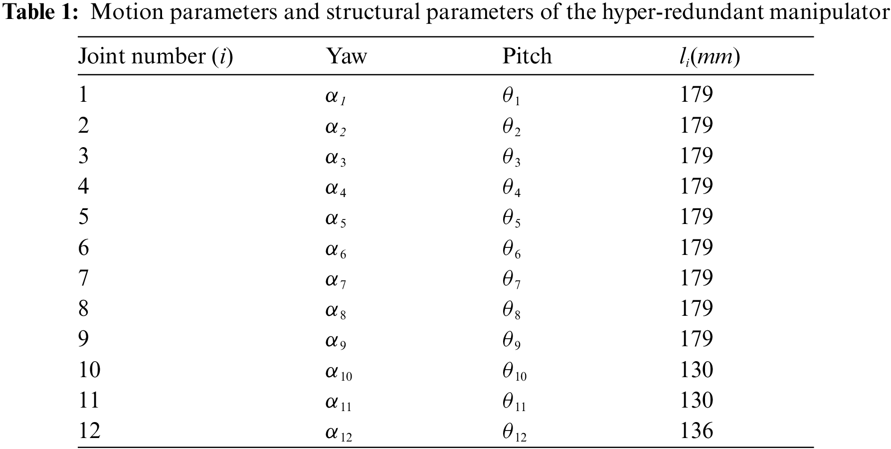
Figure 2: Universal joint coordinate systems and conversion rules between adjacent coordinate systems

The homogeneous transformation matrix used during this study is presented as

Ti−1i=Trans(0,0,li−1)Rot(y′i−1,θi)Rot(x′′i−1,αi)=[cαisαisθisαicθi00cθi−sθi0−sαicαisθicαicθiLi−10001](i=2,3,…,12),(1)

where c and s represent cosandsin, respectively.

The coordinate transformation process from the basic O0x0y0z0 coordinate system to the O0x1y1z1 coordinate system is to rotate the O0x0y0z0 coordinate system by −90∘ around the y0 axis to obtain the O0x0′y0′z0′ coordinate system, then the O0x0′y0′z0′ coordinate system must rotate 180∘ around the x0′ axis to obtain the O0x0′′y0′′z0′′ coordinate system. Then the O0x0′′y0′′z0′′ coordinate system must be rotated around the y0′′ axis by α1 to obtain the O0x0′′′y0′′′z0′′′ coordinate system. Finally, the O0x0′′′y0′′′z0′′′ coordinate system is rotated around the x0′′′ axis by θ1 to obtain the O0x1y1z1 coordinate system, as shown in Fig. 3.

Figure 3: Coordinate transformation for the coordinate system of the first joint

The homogeneous transformation matrix from the basic O0x0y0z0 coordinate system to the O0x1y1z1 coordinate system can be expressed by

T01=Rot(y0,−π/2)Rot(x0′,π)Rot(y0′′,θ1)Rot(x0′′′,α1)=[−sα1cα1sθ1cα1cθ100−cθ1sθ10cα1sα1sθ1sα1cθ100001].(2)

The transformation matrix of the ith joint is expressed by

T0i=T01T12T23…Ti−2i−1Ti−1i(i≤12).(3)

The kinematics equation for the hyper-redundant manipulator can then be expressed by

[XYZ1]=012T[00l121].(4)

When the joint angles are inserted into Eqs. (1)–(4), the position of the manipulator's end effector can be obtained.

3  Motion-Planning Algorithm Based on the Backbone Curve and Path-Following

The geometric method, based on the backbone curve, was used to solve the inverse kinematics of the hyper-redundant manipulator in this study. The backbone curve of the hyper-redundant manipulator had to be determined first. Then the positions of the hyper-redundant manipulator joints must be fitted to the backbone curve. Finally, the geometric method was used to solve for the joint angles.

3.1 Backbone Curve Based on the Mode Function

The modal method uses differential geometry to solve the inverse kinematics of hyper-redundant manipulators. The backbone curve of the mode function is shown in Fig. 4.

Figure 4: Mode function backbone curve

The mode function of the backbone curve [23] is expressed by

X(s,t)=∫0slu(σ,t)dσ=[x(s,t)y(s,t)z(s,t)],(5)

where s represents the normalized length parameter of the backbone curve and l represents the length of the backbone curve. The coordinates of each point in the backbone curve in the O0x0y0z0 coordinate system are represented by x(s,t), y(s,t), and z(s,t). u(σ,t) represents the unit tangent vector of the backbone curve at σ, and can be expressed by

u(s,t)=[sin⁡K(s,t)⋅cos⁡T(s,t)cos⁡K(s,t)⋅cos⁡T(s,t)sin⁡T(s,t)].(6)

In Eq. (6), K(s,t) and T(s,t) determine the pose of the backbone curve and are expressed by

K(s,t)=a1sin(2πs)+a2(1−cos(2πs))+b1k(1−sin(π2s))+b2ksin(π2s)T(s,t)=a3(1−cos(2πs))+b1t(1−sin(π2s))+b2tsin(π2s).(7)

In Eq. (7), a1, a2, and a3 are modal participation factors. b1k and b1t are the two angles of the initial position of the main curve corresponding to K(0,t) and T(0,t), respectively. b2k and b2t are the two angles of the end position of the main curve corresponding to K(1,t) and T(1,t), respectively. b1k, b1t, b2k, and b2t were determined by the desired angles at the beginning and end of the backbone curve.

When solving for the direction vector, u(s,t), the Newton iteration method was used to obtain the modal participation factors, a1, a2, and a3:

am+1=am+ωJa−1(am,1)[XD−Xm].(8)

In Eq. (8), ω is a constant that controls the convergence speed, m is the number of iterations, and XD is the target end position point. Xm is the end point vector of the mode function backbone curve obtained by substituting am into Eq. (7) after the mth iteration, and Ja−1(am,1) is the inverse matrix of the 3 × 3 modal Jacobian matrix when the ridge arc length, s, is equal to 1. The element relationship in Ja(a,1) is presented as

Ja(a,1)=[∂x(1,t)∂a1∂x(1,t)∂a2∂x(1,t)∂a3∂y(1,t)∂a1∂y(1,t)∂a2∂y(1,t)∂a3∂z(1,t)∂a1∂z(1,t)∂a2∂z(1,t)∂a3],(9)

where x(1,t), y(1,t), and z(1,t) are the expressions concerning the modal participation factors a1, a2, and a3, respectively, obtained when s = 1 in Eq. (5). Ja(am,1) is the 3 × 3 matrix obtained by substituting am obtained after the mth iteration into Eq. (8). When solving for the backbone curve, the backbone curve length, l, the backbone curve end point, XD, the initial point position, X0, b1k, b1t, b2k, and b2t must all be selected first. The backbone curve must be divided into Q equal parts, and the normalized coordinates of each division point are S=[0,1/Q,2/Q,…,(1−1/Q),1]. The modal participation factors, a1, a2, and a3, must be determined from Eq. (8), then they must be substituted into Eq. (5) with S as the upper limit of integration to obtain a set of mode function curves composed of Q+1 points.

3.2 New Algorithm

The motion-planning algorithm for the hyper-redundant manipulator based on path-following and the backbone curve is primarily useful for passing the end effector through curved pipes and narrow spaces.

As shown in Fig. 5, the backbone curve was divided into a mode function curve segment and a known path curve segment. Point O represents the center of the first universal joint and the AB⌢ curve is a path through a narrow space. The curve in the narrow space is defined as a known path segment (curves AE′⌢ and AE′′⌢) and the curve from the base of the manipulator to the initial point of the known path segment is defined as the mode function curve segment (curves OSA⌢, OTA⌢, and OUA⌢). The known path length was obtained by the trapezoidal integration method, expressed by

Lpath=∫0s(dxpathdt)2+(dypathdt)2+(dzpathdt)2dt.(10)

Figure 5: The motion process of the backbone curve when the new algorithm was used

In Eq. (10), the integral's upper limit is s=1. xpath, ypath, and zpath are the coordinate values of the discrete points in the path and M represents the total number of discrete points in the path. t is the normalized main curve coordinate, equal to t=[1/M,2/M,…,(M−1)/M,1].

Five primary steps were used to solve for the set of backbone curves in the motion process.

Step 1: The total length of the initial mode function curve, OSA⌢, was defined as the total length of the hyper-redundant manipulator, Lsum. The starting point of the mode function curve was set as the center of the first universal joint, and end point coincided with the initial point of the known path. The angles b1k and b1t at the starting point of the mode function curve were determined by the initial orientation of the manipulator. The two end angles, b2k and b2t, remained tangent to the known path, AB⌢, so that the improved backbone curve was always smooth. The backbone curve was obtained using the method described in Section 3.1. The step length and step number were set as λ and N, respectively.

Step 2: At the ith step, the backbone curve was composed of the new mode function curve segment, OTA⌢, and the known path curve segment, AE′⌢, that had been traversed. The length of the known path curve segment that had been traversed was iλ. The new mode function curve segment length, Lm, can be expressed by

Lm=Lsum−iλαstep(0≤αstep≤1).(11)

In Eq. (11), αstep is generally 1, but when the curvature is large it is equal to 0.98.

Step 3: If the end-actuator position, E′, fell between two adjacent given points, C(xC,yC,zC) and D(xD,yD,zD), in the known path, AB⌢, then linear interpolation was used to determine the position of the landing point, E′(xE′,yE′,zE′). If the Euclidean distance between points C and D was |CD|, then Eq. (10) was used to find the length, LAC⌢, of curve |AC|, and E′(xE′,yE′,zE′) could be obtained from Eq. (12). If E′ fell on a given point of the known path, then this point was point E′. Then the mode function curve, OTA⌢, and curve AE′⌢ were connected to obtain the backbone curve, OTAE′⌢, at the ith step.

[xE′yE′zE′]=[xCyCzC]+iλ|CD|[xD−xCyD−yCzD−zC](12)

Step 4: i=i+1 was applied, and the process was repeated, beginning with Step 2, to find the backbone curve for each step. The loop was terminated when i=N−1.

Step 5: When i=N, the step length was changed so that the position, E′′, of the manipulator's end actuator fell on the end point, B, of the known curve. Then the backbone curve could be obtained.

3.3 Fitting of the Hyper-Redundant Manipulator and the Backbone Curve

As shown in Fig. 6, a dichotomy was used to fit the end point of the manipulator and the center of each universal joint to the backbone curve in turn, in the direction from the end point to the origin. The fitting process followed four primary steps.

Figure 6: The relationship between the manipulator and the backbone curve during motion

Step 1: The initial mode function curve from the base coordinate origin of the manipulator to the starting point of the known path was composed of Q+1 known discrete points. The initial point of the backbone curve was defined as the left end point of the dichotomy iteration, and the end of the backbone curve as the right end point. The coordinates of the mth point were found, and this point was defined as point W(m=[Q/2]). When the distance from point W to the right end of the backbone curve was greater than the length of the end linkage, the right endpoint remained unchanged, and point W was taken as the left endpoint. When the distance from point W to the right end of the backbone curve was less than l12, the left endpoint remained unchanged, and point W was taken as the right endpoint. Then iterations continued with the new left and right endpoints. The iterations stopped when the distance from point W to the end point of the backbone curve was equal to the length of the end linkage within the accuracy range. If point W coincided with a known point, then this point was taken as the center point of universal joint O12. Otherwise, the two known points, Pj−1 and Pj, that were adjacent to the target point, were found.

Step 2: Pj−1 and Pj were connected to place the end point of the backbone curve at the center of a circle with l12 as the arc radius. The intersection of the arc and line Pj−1Pj was taken as O12, as shown in Fig. 7.

Figure 7: Selection of the center position of a universal joint

Step 3: Similarly, Steps 1 and 2 were repeated to fit all but the first two universal joints to the backbone curve in turn.

Step 4: When determining the position of the second universal joint, the middle vertical plane of vector O1O3→ was used to draw a sphere with O1 as the center and l1 as the radius. Circle T resulted from the intersection of the sphere and the plane. Any point on the circle was selected as O2. The fitting of the manipulator and the backbone curve is shown in Fig. 8.

Figure 8: Selection of the center position of the second universal joint

When a hyper-redundant manipulator is fitted, the length of the backbone curve must be appropriately greater than the length of the manipulator if the backbone curvature is large.

3.4 Solving for the Joint Angles

The universal joint angles for the hyper-redundant manipulator were solved using the closed vector method. In Fig. 9, On+1 represents the endpoint of the end effector. L1, L2,…, Ln denote the linkage vectors in the base coordinate system, O0x0y0z0. X2, X3,…, Xn represent the joint center vectors in the base coordinate system, O0x0y0z0, expressed as Xi=[xiyizi1]T, and Xn+1 represents the endpoint vector.

Figure 9: Closed vector model for the hyper-redundant manipulator

The process of solving for the manipulator's joint angles was divided into three primary steps [23].

Step 1: For the first universal joint, the known vector, X2, could be expressed by

X2=[x2y2z21]=T01[00l11].(13)

In Eq. (13), x2, y2, and z2 are the coordinates of the center position of the second universal joint in the base coordinate system, O0x0y0z0, and T01 is the homogeneous transformation matrix shown in Eq. (2). By solving T01, the rotation angles for the first universal joint, α1 and θ1, were obtained.

Step 2: For the second universal joint, α2 and θ2 in T12 were obtained by solving

(T01)−1[x3y3z31]=T12[00l21].(14)

Step 3: Similarly, αi and θi(i=2,3,…,12) were obtained by solving

(T0i−1)−1[xi+1yi+1zi+11]=Ti−1i[00li1].(15)

4  Engineering Experiments

4.1 Motion Through a Bent Pipe

As shown in Fig. 10, during the exploration of a certain piece of aviation equipment, the base of a hyper-redundant manipulator was at O0(0,0,0), and A(1,200,100,300mm) was the starting point of the central axis of the bent pipe. The diameter of the pipe was 70 mm, the turning radius was 100 mm, and the end point of the central axis of the pipe was located at B(1,800,100,100 mm). The red line between A and B represents the known path segment. The hyper-redundant manipulator was required to pass through the bent pipe. The inverse solution for the hyper-redundant manipulator was solved using the proposed algorithm.

Figure 10: Bent pipe model and path selection

The origin of the mode function curve was at O0 and the end point of the mode function curve was at A. Using the algorithm described in Section 3.1, the four angles, b1k, b1t, b2k, and b2t, were set as 0, 0, π/2, and 0, and Lsum was set as 2,007 mm. The mode function curve segment is shown in Fig. 11a. Also, the end effector of the hyper-redundant manipulator was made to move forward along the curved path with a 5-mm step length. The orientation of the backbone curve at the 60th step is shown in Fig. 11b. The end point of the backbone curve had traveled 300 mm along the known path. The starting point, the end point, and the four angle parameters, b1k, b1t, b2k, and b2t, of the mode function curve were the same as in Fig. 11a. In Fig. 11c, the end point of the backbone curve moved to the target position.

Figure 11: Orientation of the backbone curve during the motion through the bent pipe

When solving for the backbone curve at each step, the hyper-redundant manipulator and the backbone curve were fitted by the algorithm described in Section 3.3, and the results are shown in Fig. 12. The three hyper-redundant manipulator orientations in Fig. 12 correspond to the three backbone curves in Fig. 11, and the manipulator orientations were consistent with the backbone curves. In Fig. 12a, the manipulator was in the initial motion state. In Fig. 12b, the end effector and the 11th and 12th universal joints were located on the known path and moved along the direction tangent to the path. Fig. 12c shows that the end effector coincided with the end point B, and that the 9th–12th universal joints were close to the known path to achieve the expected motion. The inverse solutions are shown in Fig. 13.

Figure 12: Orientations of the hyper-redundant manipulator during motion

Figure 13: Inverse solutions of the hyper-redundant manipulator as it traveled through the bent pipe

The red and blue curves in Fig. 13 represent the changes in α and θ, respectively. The trends were relatively smooth. These solutions were substituted into the positive kinematics equation in Section 3.1 to drive the robot's motion. The hyper-redundant manipulator passed through the bent pipe, verifying the effectiveness of the algorithm.

4.2 Motion When Entering Narrow Cabins

As shown in Fig. 14, during the process of exploring a piece of an aviation equipment, the center of the first universal joint in the hyper-redundant manipulator was at O0(0,0,0), and it had to enter the cabins sequentially for cleaning or searching. The manipulator was directed to move along the red path to point C (1,470, −50, 200 mm), and the coordinates of A and B were (1,200, 100, 300 mm) and (1,470, 190, 300 mm), respectively.

Figure 14: Path selection and location of key points

Using the new method proposed in this study, a series of results were generated. A backbone curve was obtained and is shown in Fig. 15a. The orientation of the backbone curve at the 60th step is shown in Fig. 15b. The length of the mode function curve segment was 1,707 mm. The modal participation factors of the mode function curve were regenerated using Equation (9), and the other parameters remained unchanged. In Fig. 15c, the manipulator had reached the target point. Fig. 15d and Fig. 15e represents the backbone curve during the return motion and the backbone curve when the manipulator had returned to the starting point, respectively. The hyper-redundant manipulator and the backbone curve were fitted by the algorithm from Section 3.3, and the results are shown in Fig. 16. The five orientations of the hyper-redundant manipulator in Fig. 16 correspond to the five backbone curves in Fig. 15, and the manipulator orientations were consistent with the backbone curves. The orientations at the initial position and when the manipulator had entered the cabin along the known path are shown in Fig. 16a and Fig. 16b, respectively. At this time, the end effector and the 11th and 12th universal joints had entered the cabin.

Figure 15: Backbone curve orientations when entering the narrow cabins

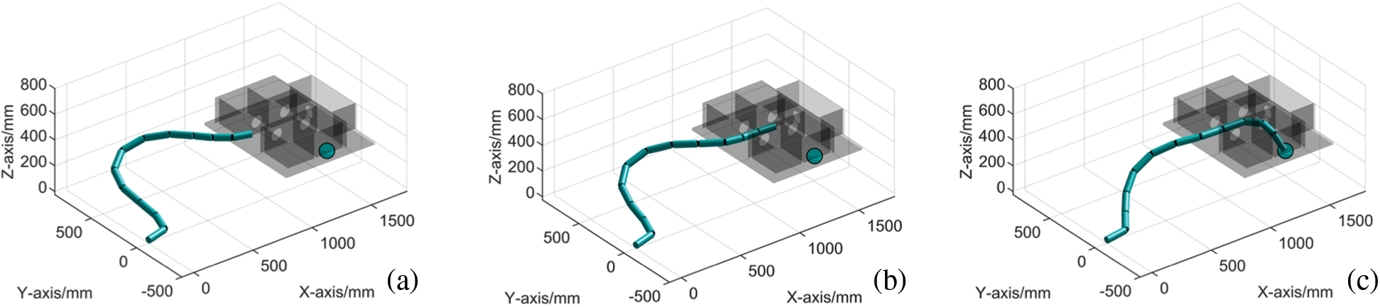
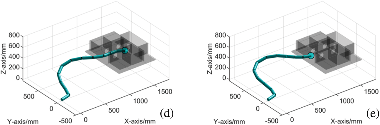
Figure 16: Manipulator orientations when entering the narrow cabins

Fig. 16c shows the orientation when the end effector had reached the end point, C. The end effector and the 11th and 12th universal joints were located in one cabin, and the 9th and 10th universal joints were located in another cabin. Fig. 16d shows that the end effector returned along the known path. Fig. 16e shows the end effector and the universal joints when the hyper-redundant manipulator had completely exited the cabins. These inverse solutions are shown in Fig. 17. Simulation experiments based on these inverse solutions verified the correctness and effectiveness of the new algorithm.

Figure 17: The angles of the universal joints and the manipulator motion when entering the narrow cabins

5  Conclusions

Using the homogeneous coordinate transformation method to derive the positive kinematics equation for a hyper-redundant manipulator can reduce the number of coordinate systems, simplify the derivation process for the transformation matrix, and save calculation time. An improved modal backbone curve method was proposed in this study. First, with changes in the discrete points along the known path, the backbone curves that the hyper-redundant manipulator used to reach these points were dynamically obtained. Then, the joints of the hyper-redundant manipulator were fitted to the modal backbone curves. Finally, the inverse kinematics of the hyper-redundant manipulator were solved based on the spatial geometry method. This method solved the motion-planning problem of an industrial hyper-redundant manipulator entering a known narrow environment.

Engineering application experiments verified the hyper-redundant manipulator's ability to move through curved pipes and narrow workspace areas. The effectiveness of the new algorithm was also proven by these experiments.

Funding Statement: The authors gratefully acknowledge the financial support provided by the National Key Research & Development Project of China (Grant No. 2019YFB1311203).

Conflicts of Interest: The authors declare that they have no conflicts of interest to report regarding the present study.

References

 1.  F. Feng, L. N. Tang and J. F. Xu, “A review of the end-effector of large space manipulator with capabilities of misalignment tolerance and soft capture,” Science China Technological Sciences, vol. 59, no. 11, pp. 1621–1638, 2016. [Google Scholar]

 2.  T. Rybus, “Obstacle avoidance in space robotics: Review of major challenges and proposed solutions,” Progress in Aerospace Sciences, vol. 101, pp. 31–48, 2018. [Google Scholar]

 3.  T. Zhang, Y. Cheng and H. P. Wu, “Dynamic accuracy ant colony optimization of inverse kinematic (DAACOIK) analysis of multi-purpose deployer (MPD) for CFETR remote handling,” Fusion Engineering and Design, vol. 156, pp. 111522, 2020. [Google Scholar]

 4.  C. Choi, A. Tesini and R. Subramanian, “Multi-purpose deployer for ITER in-vessel maintenance,” Fusion Engineering and Design, vol. 98–99, pp. 1448–1452, 2015. [Google Scholar]

 5.  Q. Zhang, “Motion control system design of multi-joint snake-like manipulator for nuclear environment,” Journal of Shandong University (Engineering Science), vol. 48, no. 6, pp. 122–131, 2018. [Google Scholar]

 6.  L. Dupourqué, F. Masaki and Y. L. Colson, “Transbronchial biopsy catheter enhanced by a multisection continuum robot with follow-the-leader motion,” International Journal of Computer Assisted Radiology and Surgery, vol. 14, pp. 2021–2029, 2019. [Google Scholar]

 7.  Y. Gao, K. Takagi and T. Kato, “Continuum robot with follow-the-leader motion for endoscopic third ventriculostomy and tumor biopsy,” IEEE Transactions on Biomedical Engineering, vol. 67, no. 2, pp. 379–390, 2020. [Google Scholar]

 8.  P. J. Swaney, A. W. Mahoney and A. A. Remirez, “Tendons, concentric tubes, and a bevel tip: Three steerable robots in one transoral lung access system,” in IEEE Int. Conf. on Robotics and Automation (ICRA), Seattle, WA, USA, pp. 5378–5383, 2015. [Google Scholar]

 9.  X. R. Zhang, X. Sun, X. M. Sun, W. Sun and S. K. Jha, “Robust reversible audio watermarking scheme for telemedicine and privacy protection,” Computers, Materials & Continua, vol. 71, no. 2, pp. 3035–3050, 2022. [Google Scholar]

10. J. Q. Peng, W. F. Xu and T. W. Yang, “Dynamic modeling and trajectory tracking control method of segmented linkage cable-driven hyper-redundant robot,” Nonlinear Dynamics, vol. 101, pp. 233–253, 2020. [Google Scholar]

11. S. Yahya and M. Moghavvemi, “Redundant manipulators kinematics inversion,” Academic Journals, vol. 6, no. 26, pp. 5462–5470, 2011. [Google Scholar]

12. J. A. Tenreiro Machado and A. M. Lopes, “A fractional perspective on the trajectory control of redundant and hyper-redundant robot manipulators,” Applied Mathematical Modelling, vol. 46, pp. 716–726, 2017. [Google Scholar]

13. I. Gravagne and I. D. Walker, “Properties of minimum infinity-norm optimization applied to kinematically redundant robots,” in Proc. 1998 IEEE/RSJ Int. Conf. on Intelligent Robots and Systems, Victoria, BC, Canada, Innovations in Theory, Practice and Applications, vol. 1, pp. 152–160, 1998. [Google Scholar]

14. F. Yin, Y. N. Wang and Y. M. Yang, “Inverse kinematics solution for robot manipulator based on neural network under joint subspace,” International Journal of Computers Communications & Control, vol. 7, no. 3, pp. 459–472, 2012. [Google Scholar]

15. P. Y. Zhang, S. Lu and B. Song, “RBF networks-based inverse kinematics of 6R manipulator,” International Journal of Advanced Manufacturing Technology, vol. 26, no. 1–2, pp. 144–147, 2005. [Google Scholar]

16. G. S. Chirikjian and J. W. Burdick, “The kinematics of hyper-redundant robot locomotion,” IEEE Transactions on Robotics and Automation, vol. 11, no. 6, pp. 781–793, 1995. [Google Scholar]

17. G. S. Chirikjian and J. W. Burdick, “A modal approach to hyper-redundant manipulator kinematics,” IEEE Transactions on Robotics and Automation, vol. 10, no. 3, pp. 343–354, 1994. [Google Scholar]

18. J. G. Wang, L. Tang and G. Y. Gu, “Tip-following path planning and Its performance analysis for hyper-redundant manipulators,” Journal of Mechanical Engineering, vol. 54, no. 3, pp. 18–25, 2018. [Google Scholar]

19. X. R. Zhang, W. F. Zhang, W. Sun, X. M. Sun and S. K. Jha, “A robust 3-D medical watermarking based on wavelet transform for data protection,” Computer Systems Science & Engineering, vol. 41, no. 3, pp. 1043–1056, 2022. [Google Scholar]

20. Y. Han, H. Zhang, Z. Shi and S. Liang, “An adaptive fuzzy control model for multi-joint manipulators,” Computer Systems Science and Engineering, vol. 40, no. 3, pp. 1043–1057, 2022. [Google Scholar]

21. I. Al-Darraji, A. A. Kakei, A. G. Ismaeel, G. Tsaramirsis and F. Q. Khan et al., “Takagi–sugeno fuzzy modeling and control for effective robotic manipulator motion,” Computers, Materials & Continua, vol. 71, no. 1, pp. 1011–1024, 2022. [Google Scholar]

22. S. B. Andersson, “Discretization of a continuous curve,” IEEE Transactions on Robotics, vol. 24, no. 2, pp. 456–461, 2008. [Google Scholar]

23. F. Fahimi, H. Ashrafiuon and C. Nataraj, “An improved inverse kinematic and velocity solution for spatial hyper-redundant robots,” IEEE Transactions on Robotics and Automation, vol. 18, no. 1, pp. 103–107, 2002. [Google Scholar]

This work is licensed under a Creative Commons Attribution 4.0 International License, which permits unrestricted use, distribution, and reproduction in any medium, provided the original work is properly cited.