DOI:10.32604/cmc.2022.025206
| Computers, Materials & Continua DOI:10.32604/cmc.2022.025206 | |
| Article |
Modelling the ZR Relationship of Precipitation Nowcasting Based on Deep Learning
1Chengdu University of Information Technology, Chengdu, 610225, China
2Bournemouth University, Bournemouth, BH12 5BB, UK
*Corresponding Author: Jianbing Ma. Email: mjb@cuit.edu.cn
Received: 16 November 2021; Accepted: 07 January 2022
Abstract: Sudden precipitations may bring troubles or even huge harm to people's daily lives. Hence a timely and accurate precipitation nowcasting is expected to be an indispensable part of our modern life. Traditionally, the rainfall intensity estimation from weather radar is based on the relationship between radar reflectivity factor (Z) and rainfall rate (R), which is typically estimated by location-dependent experiential formula and arguably uncertain. Therefore, in this paper, we propose a deep learning-based method to model the ZR relation. To evaluate, we conducted our experiment with the Shenzhen precipitation dataset. We proposed a combined method of deep learning and the ZR relationship, and compared it with a traditional ZR equation, a ZR equation with its parameters estimated by the least square method, and a pure deep learning model. The experimental results show that our combined model performs much better than the equation-based ZR formula and has the similar performance with a pure deep learning nowcasting model, both for all level precipitation and heavy ones only.
Keywords: Deep learning; meteorology; precipitation nowcasting; weather forecasting; ZR formula
Nowcasting has always played an important role in the field of weather forecast. Whilst it also works in predicting phenomenons such as lightning [1], Hailstorm [2], convective storm [3–5], straight-line convective wind [6] and tropical cyclone [7], most of the nowcasting efforts are applied to forecasting precipitation. Traditionally, precipitation nowcasting methods were generally based on weather radar extrapolation, or physical-numerical models on precipitation processses (among which the Numerical Weather Prediction (NWP) model that utilizes high-resolution data increased in popularity), or the combination of the two (i.e., knowledge-based expert systems [8]). NWP performs well on minute-level prediction and day-level forecasting, leaving the middle level (i.e., 1–2 h) not as well predicted as the two ends. Whilst the traditional NWP technique had been proved to be infeasible in precipition nowcasting [9,10], the linear extrapolation methods [11,12] were then introduced and showed better performance than NWP. However, these methods could not capture the underlying patterns of aberrations and trends from the historical data as the dynamic and non-linear nature of nowcasting. So nowadays, scientists have been beginning to deploy deep neural networks [10,11,13,14] to deal with the spatio-temporal inputs of precipitation nowcasting, such as Long Short-Term Memory (LSTM) [13,14], Gated Recurrent Unit (GRU) [15], 3-Dimensional Convolutional Neural Network (3D-CNN) [10], and the recent Transformer model which is based on the attention mechanism [11], were widely used in the applications. The drawback of the deep learning models might be that they are not easily understood, especially for those working in the meteorology area.
The relationship between radar reflectivity (Z) and precipitation (R) also plays an important role in predicting precipitation in the literature. Many experiments directly used the ZR formula (Z = aRb) derived from the data to predict rainfall rates according to the Z values [16,17], dating back to the Marshall-Palmer formula [18] (Z = 200 R1.6 where Z is in mm6/m3 and R is in mm/h) which links radar reflectivity and precipitation rate. Although the formula was intensively used, it comes with arguably uncertainty, as the values of the parameters are usually estimated through an empirical approach, based on the comparison of radar and rain gauge. People argue that an improper selection of the parameters (for instance the conventional setting a = 200 and b = 1.6) may lead to a bad prediction.
There were quite a few efforts proposed to improve the ZR relation, for instance, [12,19] tried to introduce additional features to reduce the estimation error, such as type of precipitation, distance from the radar, etc., while [20–22] added seasonal, monthly, or multi-daily time scale feature information. However, these features are not always available, and the results are not universally better than that of the simple ZR formula.
To this end, in this paper, we propose a deep learning-based method to model the ZR relation. That is, we incorporate the estimation of the parameters of the ZR relationship into a deep learning model. By having such a model, we do not need to introduce additional features like in [12,19–22], so the model can be universally used in different regions and time scales. To evaluate its performance, we compared our result to those of equation-based ZR models and a pure deep learning network. The experiment shows that our model performs much better than the equation-based models and has the similar performance with the pure deep learning one, while our model is much easier to be understood by meteorologists than the deep learning model.
The rest of the paper is organized as follows. Section 2 introduces the dataset, followed by Section 3 that provides the example design details. In Section 4, we discuss and evaluate our model performance. Finally, Section 5 concludes the paper.
We used a dataset containing real radar images and precipitation rate at the target sites, which were collected by the Meteorological Observation Center of Shenzhen.
The characteristics of a typical sample of the dataset is as follows:
1. Each radar image contains a target site (located in the center of the image);
2. Each radar image contains the total amount of precipitation at the target site for the time interval of the next 1 to 2 h. Here we should note that it does not provide the amount of precipitation for the next hour;
3. In each sample, there are four groups of images, each of which contains 15 radar images of a successive time period. Each two adjacent images come with an interval of 6 min. Each group of radar images were measured at the same area but at a different height, with an interval of 1 km, ranging from a distance of 0.5 to 3.5 km;
4. According to the latitude and longitude of the target location, each radar image covers an area of 101 × 101 square kilometers. The area is marked as 101 × 101 grids (with the starting index as 0 for each coordinate), and the target position is in the center, that is, with a coordinate (50, 50).
Since each sample contains radar echo maps of 4 heights and covers 15 time points, it has a dimension (15, 4, 101, 101).
The following Fig. 1 is an example of a visualization of radar echo data for a given sample at a given height. From left to right and top to bottom are arranged in chronological order. Above each graph is the average pixel value (average of reflected echo intensity) for that graph. From left to right and top to bottom are arranged in a chronological order. The average pixel value (average of reflected echo intensity) for that plot is shown above each plot, with row being the sample ordinate, high being the height ordinate, and rain being the precipitation amount.
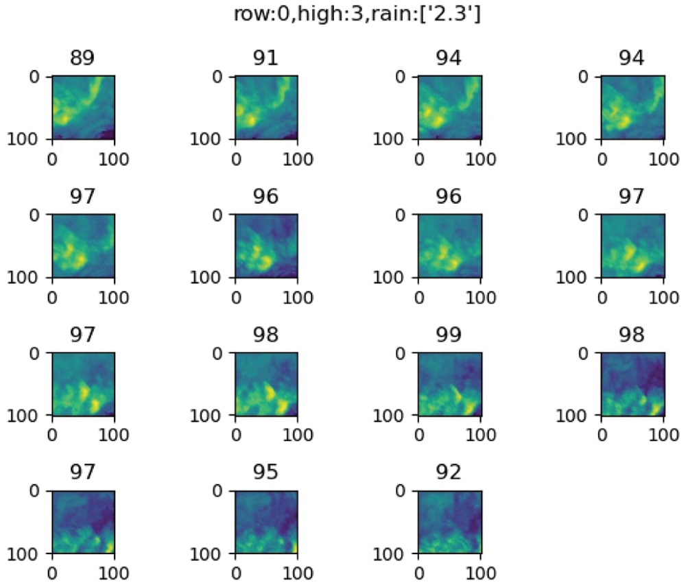
Figure 1: An example of the radar echo maps coming from the fourth altitude
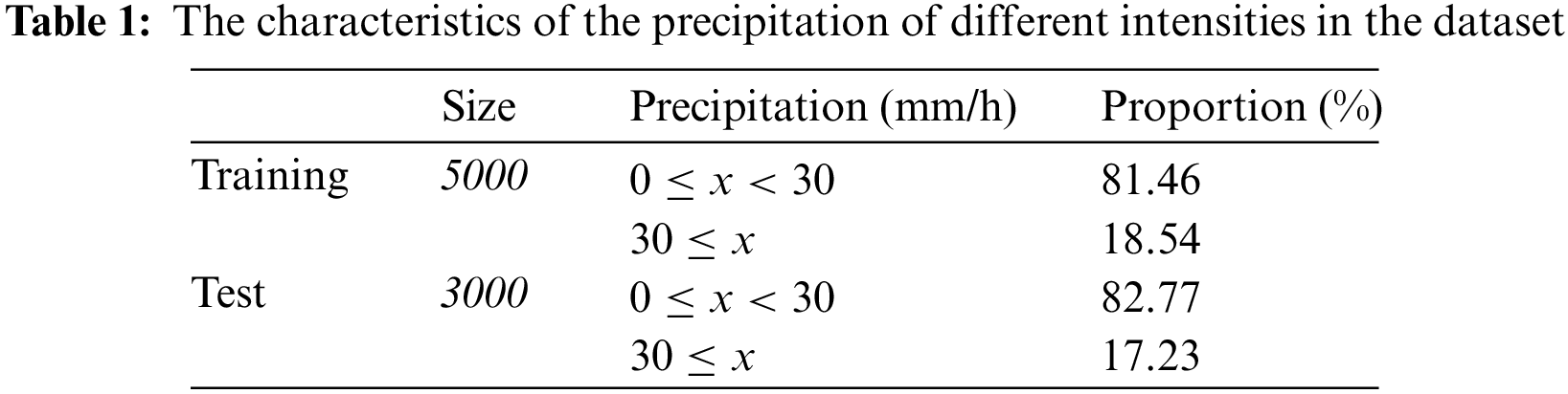
In the dataset, there are 5000 training samples and 3000 testing samples, with around 18% heavy precipitation samples (>30 mm/h), as shown in Tab. 1 below.
In our experiments, we chose the radar echo data at the fourth altitude (3.5 km) for training due to its higher prediction accuracy at this altitude. In our experiments concerning deep learning, the general idea is to use CNN to extract features from the radar images, and then use the Transformer blocks to process the features in a temporal order.
In summary, here we present four experiments to model the relation between the radar reflectivity factor (Z) and rainfall rate (R):
Case 1: We used the direct ZR formula Z = a * Rb. Two parameter settings were used. The first pair of a and b in the ZR formula is the traditional one i.e., a = 200, b = 1.6, while the second pair of a and b are fitted using the least square method from the training data, and they were a = 0.3, b = 2.6.
Case 2: We fitted the ZR relation into a deep learning model, so as to combine human knowledge and deep learning algorithms. The model hence relies on the existing mathematical equation to shape the deep learning model to reduce the potential overfitting problem.
Case 3: To compare, here we also proposed a pure deep learning model to predict the precipitation amount. We used a model that contains CNN, Transformer, and fully connected neural network blocks.
3.1 The Direct ZR Formula Case
As mentioned above, we have used two parameter settings for a and b in the formula. Since the geographical area of the radar echo map is too large, we intercepted the 15*15 area in the center of the radar map for the Z values, as indicated by Fig. 2 below.
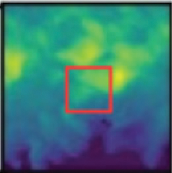
Figure 2: The interception of the central area of the radar echo map for the Z values
With the dataset setting, we then transformed the pixel values into the dbz values as follows:
The dbz values were converted into Z values by the equation:
Finally, we took the average Z-values of the central 15*15 region to be used in the ZR formula, i.e.,
With the Z values and the corresponding R values, we use the least square method to train the parameters, and get a = 0.3, b = 2.6.
3.2 The CNN + LSTM + FC + ZR Case
In this model, we fit the ZR relation into a deep learning model that contains CNN, LSTM, and fully connected neural network blocks, as indicated by Fig. 3.
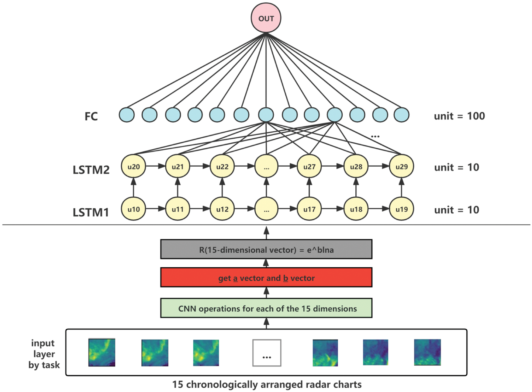
Figure 3: The ZR relation fitted deep learning model
Note that the equation Z = a*Rb can be converted into:
We replace 1/b and z/a in the above figure with b2 and a2 respectively, and we get:
With Eq. (6), we introduce a deep learning model to train the parameters a2 and b2 instead of simply fitting them by the least square method as in case 1. The parameters obtained in this way are hence spatially and temporally characterized and can be dynamically adjusted according to the radar image characteristics to obtain more flexible prediction values.
The model structure of the CNN block used to extract feature maps is illustrated in the following two figures (Fig. 4 and Fig. 5).
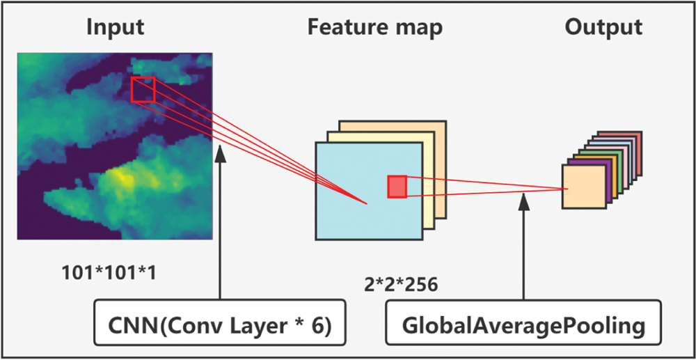
Figure 4: The model structure of the CNN block
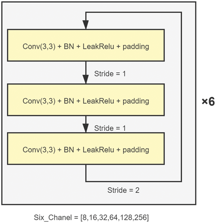
Figure 5: The convolution layer used in the CNN block
In the CNN block, six convolution layers of the same structure are used (as shown in yellow in Fig. 5) to extract features, which are then compressed and output by a GlobalAveragePooling layer.
3.3 The CNN + Transformer + FC Case
To compare, in this subsection, we propose a pure deep learning model to predict the precipitations. In this model, we use the transformer network to replace the working part of LSTM. The transformer block has no recursion and convolution, and its ability to process time series is entirely due to its attention mechanism. It has been shown in [11] that the transformer block has a higher accuracy and efficiency than that of LSTM on many natural language tasks.
In our experiment, we made a few changes to the transformer block in [11] such that we remove the decoding layer of transformer since in our scenario we only need the encoding layer to get the location feature vectors, and temporal features are obtained by adding position encoding and attention mechanisms to each graph.
The model structure is illustrated by the following Fig. 6.
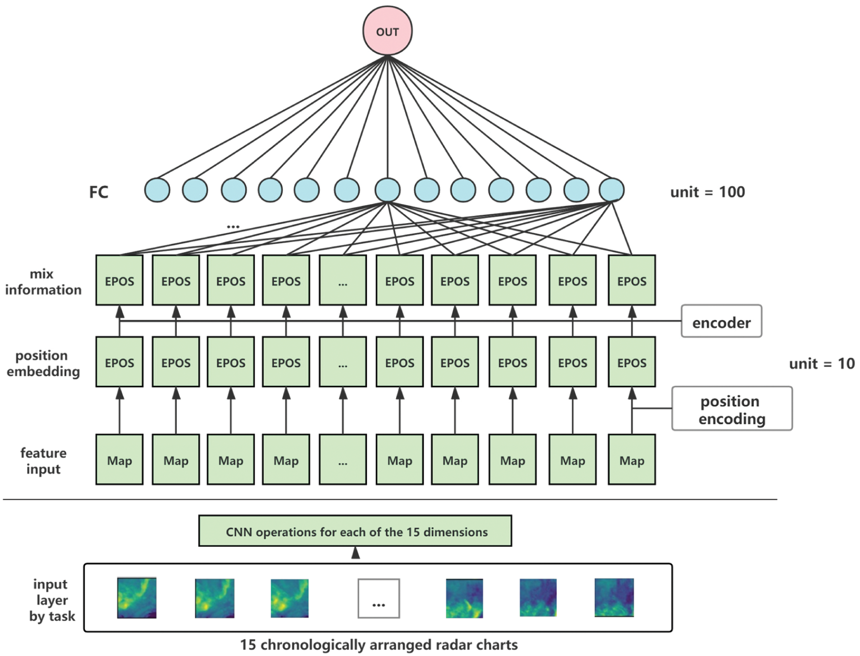
Figure 6: The model structure with transformer
In this section, we evaluate the effectiveness of the ZR relation based models and the pure deep learning model on precipitation prediction. The RMSE losses of the models on test sets are presented in Tab. 2.
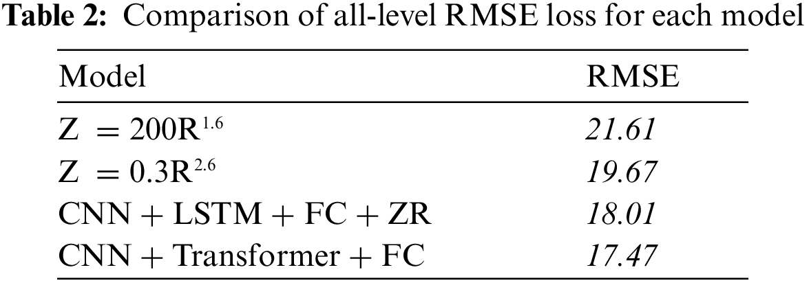
It can be found that the pure deep learning model performs the best, while the deep learning + ZR combined model gives an RMSE 18.01 which is very close to the best result (17.47), and is much better than those of the traditional ZR relationship
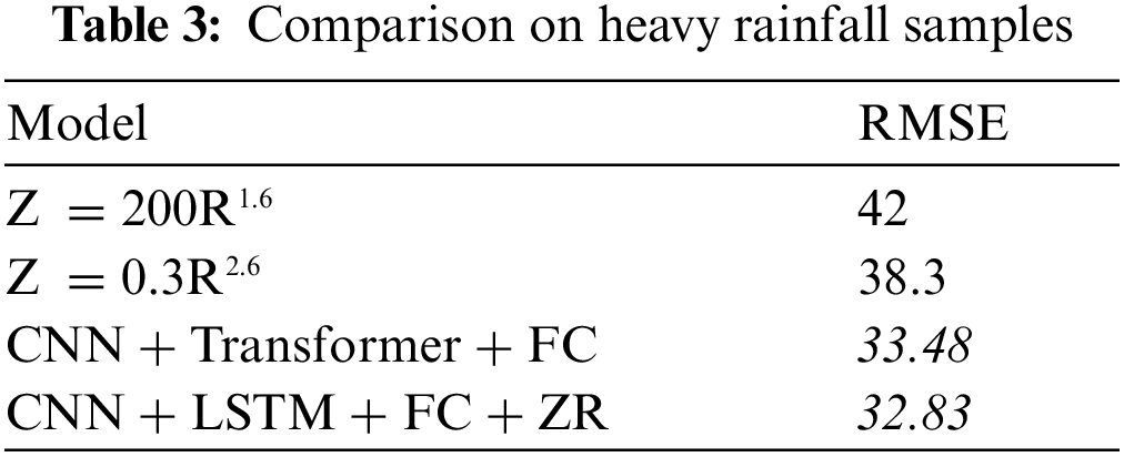
The same phenomena also appear in Tab. 3, where we focus on heavy rainfall (precipitation samples >30 mm/h) samples since in reality people are usually only concerned about heavy rainfalls.
As an illustration, here we present how these four models behave on the samples.
Fig. 7 shows the predicted rainfall rates for each model. The green horizontal line is the comparison line for rainfall rate = 30 mm/h. The vertical coordinate is the rainfall rate, and the blue bar is the predicted rainfall value and the red bar is the true value.
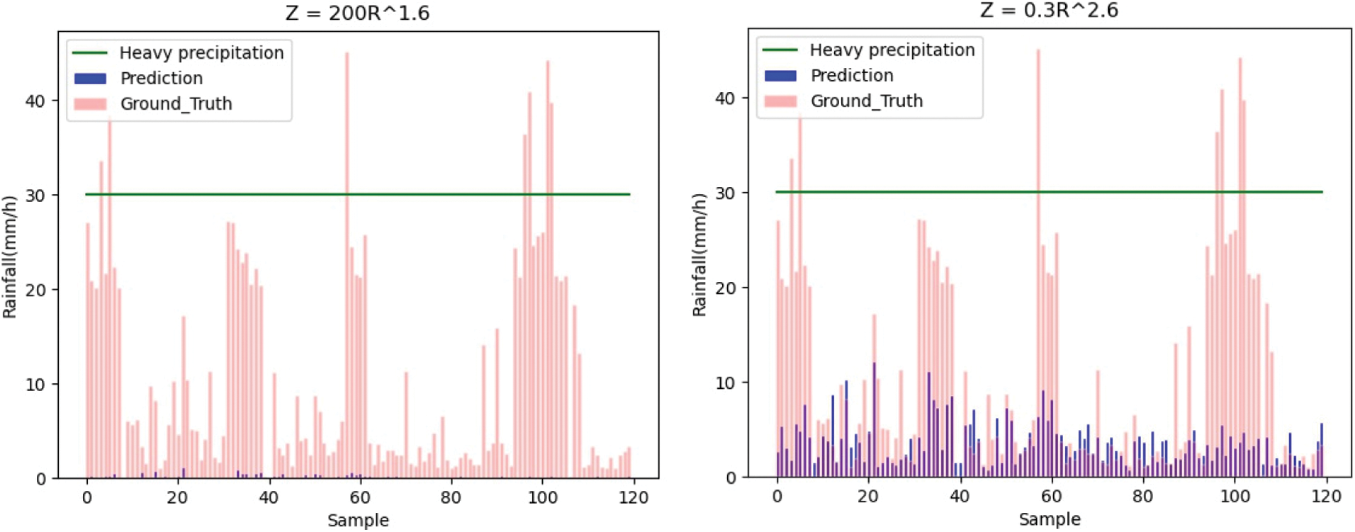
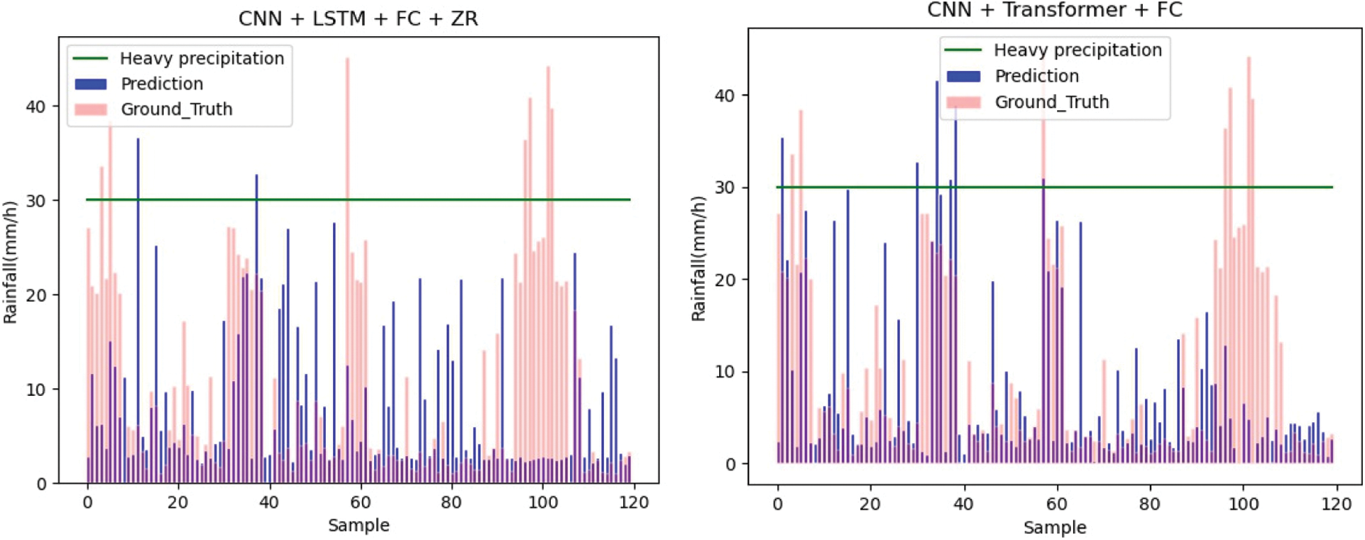
Figure 7: Precipitation prediction for each model
From the visualized rainfall rate histogram, we can clearly see that the accuracy of the deep learning model is higher than the equation-based ZR relationships, which suggests the equation-based ZR relationship might be too simple to model real precipitation, while the deep learning model can learn more features, so the performance is better than the ZR relationship. The combination of the two also performs well and improves the accuracy over the equation-based ZR model. We should also notice that for some very concentrated heavy rainfalls, for instance the ones around the 100th sample, are hardly predicted. This may imply that there should be special improvements needed for those concentrated heavy rainfalls.
Overall, our result suggests that a combination of deep learning and the traditional ZR relationship can perform similar accurate results to a pure deep learning model whilst in the meantime inherit part of the explainability of the ZR relationship, and hence could be a suitable choice for meteorologists.
In this paper, we studied how to model the ZR relationship with the help of deep learning methods. We compared a traditional ZR equation, a ZR equation with its parameters estimated by the least square model, a combined deep learning and ZR relation model, and a pure deep learning model with a meteorological dataset from Shenzhen, and found that the combined model had a similar performance to the pure deep learning model, and both models performed much better than the equation-based models. The same conclusion also holds if we focus on heavy precipitations only.
As a future work, we will try to introduce more methods to cope with the ZR relation, such as the rough set model [23], the spatio-temporal network [24,25], and methods employed in visual tracking [26]. We will also check if our conclusion can be applied to other datasets such as [27] to increase the credibility of the conclusion. A special consideration for concentrated heavy rainfalls will also be studied further.
Acknowledgement: We would like to thank Prof. Xi Wu and Ms. Yanfei Xiang for their great support and helpful suggestions to the paper.
Funding Statement: This work is supported by Sichuan Provincial Key Research and Development Program (No. 2021YFG0345, to J. Ma) and the National Key Research and Development Program of China (No. 2020YFA0608001, to J. Ma).
Conflicts of Interest: The authors declare that they have no conflicts of interest to report regarding the present study.
1. K. Zhou, Y. Zheng, W. Dong and T. Wang, “A deep learning network for cloud-to-ground lightning nowcasting with multisource data,” Journal of Atmospheric and Oceanic Technology, vol. 37, no. 5, pp. 927–942, 2020. [Google Scholar]
2. D. Gagne, S. Haupt, D. Nychka and G. Thompson, “Interpretable deep learning for spatial analysis of severe hailstorms,” Monthly Weather Review, vol. 147, no. 8, pp. 2827–2845, 2019. [Google Scholar]
3. L. Jiang, W. Zhang and L. Han, “Strong convective storm nowcasting using a hybrid approach of convolutional neural network and hidden markov model,” in Ninth Int. Conf. on Graphic and Image Processing, Qingdao, China, pp. 113–119, 2017. [Google Scholar]
4. L. Han, J. Dai, W. Zhang, C. Zhang and H. Feng, “A deep belief network approach using vdras data for nowcasting,” in Proc. SPIE 10615, Ninth Int. Conf. on Graphic and Image Processing (ICGIP), Qingdao, China, pp. 126–132, 2017. [Google Scholar]
5. W. Zhang, W. Li and L. Han, “A three-dimensional convolutional-recurrent network for convective storm nowcasting,” in Proc. of the ICBK, Beijing, China, 2019. [Google Scholar]
6. R. Lagerquist, A. Mcgovern and T. Smith, “Machine learning for realtime prediction of damaging straight-line convective wind,” Weather and Forecasting, vol. 32, no. 6, pp. 2175–2193, 2017. [Google Scholar]
7. S. Gao, P. Zhao, B. Pan, Y. Li, M. Zhou et al., “A nowcasting model for the prediction of typhoon tracks based on a long short term memory neural network,” Acta Oceanologica Sinica, vol. 37, no. 5, pp. 8–12, 2018. [Google Scholar]
8. J. Sun, M. Xue, J. Wilson, I. Zawadzki and S. Ballard, “Use of nwp for nowcasting convective precipitation: Recent progress and challenges,” Bulletin of the American Meteorological Society, vol. 95, no. 95, pp. 409–426, 2014. [Google Scholar]
9. R. Prudden, S. Adams, D. Kangin, N. Robinson, S. Ravuri et al., “A review of radar-based nowcasting of precipitation and applicable machine learning techniques,” arXiv preprint arXiv:2005.04988, 2020. [Google Scholar]
10. M. Patel, A. Patel and D. Ghosh, “Precipitation nowcasting: Leveraging bidirectional lstm and 1d cnn,” arXiv preprint arXiv:1810.10485, 2018. [Google Scholar]
11. A. Vaswani, N. Shazeer, N. Parmar, J. Uszkoreit, C. Jones et al., “Attention is all you need,” in Advances in Neural Information Processing Systems, Montreal, Canada, pp. 5998–6008, 2017. [Google Scholar]
12. M. Borga, E. Anagnostou and E. Frank, “On the use of real-time radar rainfall estimates for flood prediction in mountainous basins,” Journal of Geophysical Research Atmosphere, vol. 105, pp. 2269–2280, 2000. [Google Scholar]
13. X. Shi, Z. Chen, H. Wang, D. Yeung, W. Wong et al., “Convolutional LSTM network: A machine learning approach for precipitation nowcasting,” in Advances in Neural Information Processing Systems, Long Beach, California, USA, pp. 802–810, 2015. [Google Scholar]
14. S. Hochreiter and J. Schmidhuber, “Long short-term memory,” Neural Computation, vol. 9, no. 8, pp. 1735–1780, 1997. [Google Scholar]
15. X. Shi, Z. Gao, L. Lausen, H. Wang, D. Yeung et al., “Deep learning for precipitation nowcasting: A benchmark and a new model,” arXiv preprint arXiv:1706.03458, 2017. [Google Scholar]
16. C. Wei and C. Hsu, “Extreme gradient boosting model for rain retrieval using radar reflectivity from various elevation angles,” Remote Sensing, vol. 12, no. 2203, pp. 1–21, 2020. [Google Scholar]
17. E. Anagnostou and W. Krajewski, “Real-time radar rainfall estimation. Part I: Algorithm formulation,” Journal of Atmospheric and Oceanic Technology, vol. 16, pp. 189–197, 1999. [Google Scholar]
18. E. Anagnostou and W. Krajewski, “Real-time radar rainfall estimation. Part II: Algorithm formulation,” Journal of Atmospheric and Oceanic Technology, vol. 16, pp. 198–205, 1999. [Google Scholar]
19. C. Pathak and R. Teegavarapu, “Utility of optimal reflectivity-rain rate (Z-R) relationships for improved precipitation estimates,” in Proc. of the World Environmental and Water Resources Congress, Providence, RI, USA, pp. 4681–4691, 2010. [Google Scholar]
20. D. Seo and J. Breidenbach, “Real-time correction of spatially nonuniform bias in radar rainfall data using rain gauge measurements,” Journal of Hydrometeorology, vol. 3, pp. 93–111, 2002. [Google Scholar]
21. S. Rendon, B. Vieux and C. Pathak, “Continuous forecasting and evaluation of derived Z-R relationships in a sparse rain gauge network using NEXRAD,” Journal of Hydrology Engineering, vol. 18, pp. 175–182, 2013. [Google Scholar]
22. A. Libertino, P. Allamano, P. Claps and R. Cremonini, “Radar estimation of intense rainfall rates through adaptive calibration of the Z-R relation,” Atmosphere, vol. 6, pp. 1559–1577, 2015. [Google Scholar]
23. A. F. Oliva, F. M. Pérez, J. V. Berná-Martinez and M. A. Ortega, “Non-deterministic outlier detection method based on the variable precision rough set model,” Computer Systems Science and Engineering, vol. 34, no. 3, pp. 131–144, 2019. [Google Scholar]
24. S. Wang, X. Yu, L. Liu, J. Huang, T. H. Wong et al., “An approach for radar quantitative precipitation estimation based on spatiotemporal network,” Computers, Materials & Continua, vol. 65, no. 1, pp. 459–479, 2020. [Google Scholar]
25. Z. Li, J. Zhang, K. Zhang and Z. Li, “Visual tracking with weighted adaptive local sparse appearance model via spatio-temporal context learning,” IEEE Transactions on Image Processing, vol. 27, no. 9, pp. 4478–4489, 2018. [Google Scholar]
26. Z. Li, W. Wei, T. Zhang, M. Wang, S. Hou et al., “Online multi-expert learning for visual tracking,” IEEE Transactions on Image Processing, vol. 29, pp. 934–946, 2020. [Google Scholar]
27. R. Tao, Y. Zhang, L. Wang, P. Cai and H. Tan, “Detection of precipitation cloud over the tibet based on the improved u-net,” Computers, Materials & Continua, vol. 65, no. 3, pp. 2455–2474, 2020. [Google Scholar]
 | This work is licensed under a Creative Commons Attribution 4.0 International License, which permits unrestricted use, distribution, and reproduction in any medium, provided the original work is properly cited. |