DOI:10.32604/cmc.2022.024103
| Computers, Materials & Continua DOI:10.32604/cmc.2022.024103 | |
| Article |
A Two-Tier Framework Based on GoogLeNet and YOLOv3 Models for Tumor Detection in MRI
1Department of Software, Sejong University, Seoul, 05006, Korea
2Institute of Computer Sciences & Information Technology, The University of Agriculture, Peshawar, 25130, Pakistan
3College of Technological Innovation, Zayed University, Dubai, 19282, UAE
4Department of Software, Korea Aerospace University, Seoul, 10540, Korea
5Faculty of Computer Science and Engineering, Galala University, Suez, 435611, Egypt
6Information Systems Department, Faculty of Computers and Artificial Intelligence, Benha University, Banha, 13518, Egypt
7Chitkara University Institute of Engineering & Technology, Chitkara University, Rajpura, 140401, India
*Corresponding Author: Dongho Song. Email: dhsong@kau.ac.kr
Received: 04 October 2021; Accepted: 18 November 2021
Abstract: Medical Image Analysis (MIA) is one of the active research areas in computer vision, where brain tumor detection is the most investigated domain among researchers due to its deadly nature. Brain tumor detection in magnetic resonance imaging (MRI) assists radiologists for better analysis about the exact size and location of the tumor. However, the existing systems may not efficiently classify the human brain tumors with significantly higher accuracies. In addition, smart and easily implementable approaches are unavailable in 2D and 3D medical images, which is the main problem in detecting the tumor. In this paper, we investigate various deep learning models for the detection and localization of the tumor in MRI. A novel two-tier framework is proposed where the first tire classifies normal and tumor MRI followed by tumor regions localization in the second tire. Furthermore, in this paper, we introduce a well-annotated dataset comprised of tumor and normal images. The experimental results demonstrate the effectiveness of the proposed framework by achieving 97% accuracy using GoogLeNet on the proposed dataset for classification and 83% for localization tasks after fine-tuning the pre-trained you only look once (YOLO) v3 model.
Keywords: Tumor localization; MRI; Image classification; GoogLeNet; YOLOv3
Medical Image Analysis (MIA) has been one of the most interesting and active fields in the computer vision domain since the last decade. For patient treatment, the formed medical images are necessary to investigate the problems for proper diagnosis [1]. The radiology unit is responsible for biomedical image procurement using various types of machines such as computed tomography, ultrasound machine, X-ray, PET, and MRI [1,2]. The formed images taken by these radiology machines may have sharpness, illumination, or noise problems. To decrease such problems, some processing techniques of digital images are applied to optimize the formed image quality [3]. The region of interest (ROI) from the optimized images are obtained and further proceeded to calculate and identify the type, size, and stage of tumor based on 3D and 4D computer graphic algorithms [4,5].
The detection of tumors is a difficult and time-consuming task for physicians. However, the recognition of the tumor types in an effective manner without having an open brain surgery becomes possible using MRI. The concept of MRI has been used since it had many physiologically authoritative links to understand different tissues and improve the evaluation of multiple undertakings tissues configured within the diffuse tumor. However, Multiple MRI procedures segregate the tumor of low grade from the glioblastoma (Grade-IV) in addition to diffusion weighting images, the MR spectroscopy, and the perfusion weighting images. From the literature discussed in related work, it has been upheld that the MRI scans are kept in exception, particularly for the cure of human brain gliomas and biopsies of radiotherapy in numerous patients. The diagnosis of brain tumors from MRI is very significant and effective, which can tend to develop classification procedures for multiple selected human brain data and result in a lesser amount of open surgeries [6,7]. In MRI, digital imaging and communications in medicine (DICOM) and volumetric images are formed where every slice of the image is important to analyze, but it is a tedious job for the medical experts. For this reason, a system is needed to separate all the non-tumor and tumor-affected slices automatically. It is very important to diagnose the tumor in its early stage and start treatment as it may take life to a dangerous position. Therefore, to detect tumors and recognize their type, a deep learning technology, i.e., convolution neural network (CNN), is widely used [2,4].
The main challenging aspect in human brain tumor classification is the lack of data that is not available publicly, such as the RIDER data set [8], 71 MR images [9], and BraTS 2013 [10]. Another key issue with the state-of-the-art methods for human brain tumors is the absence of efficient classifiers with significantly higher accuracies. The problem of efficiency is the usage of features that are further processed using classifiers, i.e., the features are not representative enough to be trusted in real-world scenarios. For example, the classifiers trained using traditional handcrafted features such as LBP, HOG etc., can fit well to the training and testing data of the same dataset, but the classifier trained using these features cannot be generalized to unseen real-world data. In addition, smart and easily implementable approaches are unavailable in 2D and 3D medical images, which is the main problem in detecting the tumor. In this research work, a technique is innovated to detect a tumor in MRI based on accurate image processing and deep learning techniques. Image processing methods are used to optimize image quality and obtain texture and geometric information [11]. A CNN-based deep learning algorithm is used to identify that the MRI of the brain has the tumor slices or not [7,12]. The CNN model can identify the clear and tumor-infected image if it is trained on this type of image [4]. Therefore, the proposed framework is trained using our newly created dataset, collected from real-world scenarios, therefore, posing substantially improved generalization potentials against the state-of-the-art. In addition, the most suitable parameters are identified for processing CNN model. The key contributions of this study are summarized below.
• One of the major challenges in brain tumor detection is the lack of publically available and well-annotated datasets due to the confidentiality of the patients. We introduce a well-annotated brain tumor dataset comprised of MRI for the utilization and proper use in validation and training.
• A preprocessing module based on different techniques with various parameters is efficiently utilized to make the proposed model more transformative with less noise and fill the data availability gap.
• The proposed two tiers framework is based on deep learning models: GoogLeNet and YOLOv3 model. The GoggleNet model is precisely used to segregate and classify the MRI to find a tumor in images. In addition, the YOLOv3 model is employed to expedite the process of automatic fetching and localizing tumors in MRI.
The rest of the paper is organized as follows. Section 2 presents the related work about tumor detection in MRI. Section 3 explains the technical details of the proposed model for brain tumor classification and localization. Section 4 provides the experimental results of the proposed system. Finally, the conclusions and future work are explained in Section 5.
MIA has been an excited and challenging research field for the last two decades. It has many applications in different healthcare domains to investigate and diagnose patients [13]. A novel model for clinical programming is presented to deal with the division calculation of different stages [14]. This calculation helps to differentiate different tissue images from reverberation images. Researchers have clarified various methods for image processing [15]. The orthopedic specialists of Seattle (OSS) were utilized for 3D dynamic shape [16]. However, the discontinuity of the 3D dynamic form is an action of district rivalry and dynamic geodesic shape. A device based on a division technique of self-loader is presented to examine MRI and CT Images [17]. The client who needs more information can undoubtedly utilize this device because it effectively divides the image for more investigation. The existing work estimates the distinctive solo grouping calculations: Gaussian blend model, K-implies, fluffy methods, and Gaussian shrouded irregular field [18]. To consequently perceive the class of tumor, a programmed division strategy was utilized, which deals with a measurable methodology using tissue likelihood maps. This existing technique is evaluated using two tumor-related datasets. The generated results illustrate that the presented technique improved the detection performance and is recommended for programmed mind tumor division. The author proposed a novel method that can identify the type and grade of the tumor [19]. This system is examined using the information of 98 cerebrum tumor patients. The classifier utilized in the existing system is a two-fold support vector machine (SVM) which achieved an accuracy of 85%. A method of unique division calculations is presented for the division of cerebrum tumors [20]. However, this approach may not produce better outcomes due to complex dependencies among modules. A new technique for cerebrum division from MRIs is presented using mathematical dynamic shape models [21]. In this system, the issue of the limit surge was resolve and less delicate to fixation comparability.
A classification model based on four clustering methods (GMM, FCM, K-means, and GHMM) is evaluated for brain tumor detection [22]. This model employed a probabilistic approach to classify brain tumors consequently. This model is evaluated using BRATS 2013 cerebrum tumor dataset and produced reasonable accuracy for tumor classification. Another existing model used three different kinds of brain tumors MR images [23]. The information extracted from these images is used to train and test the classifiers. A machine learning-based approach is presented for brain image classification and brain structure analysis [24]. First, Discrete Wavelet Transform (DWT) is applied to break down the tumor image. The surface features from the weak images are extracted to prepare the classifier. However, this approach is complex for real implementation. A semi-automatic segmentation model is proposed for brain tumor images [25]. This model uses the arrangement of T1W for the segmentation of 3D MRIs. A framework based on CNN is presented for breast cancer images classification [26]. The structure of this existing model is intended to mine data from fitting scales. The results show that the accuracy of CNN is higher than SVM. The authors employed an available online dataset and revealed that the extracted features using deep learning with an ensemble approach could efficiently enhance the performance of classification [27]. They also showed that the SVM classifier and the RBF kernel could give better yields than the other classifiers in the perspective of the large datasets. A new method is proposed based on the CNN model to extract and classify features to identify tumor types [28]. This existing system utilized normal and abnormal MR images. The main advantage of this model is to easily utilize for MR images classification and tumor detection. A new approach is presented using the T1-weighted technique with benchmark CE-MRI datasets [29]. This approach does not utilize any handcrafted features and classifies the MR images in 2D perspectives due to the nature of the CNN model. Another classification method is presented to classify the MR images [30]. This existing system used a pre-trained model with ResNet50, VGG-16, and Inception v3 for image classification. The results of this model show that the VGG-16 achieved the highest accuracy for detection and classification. A YOLOv2-inceptionv3 model is presented for the classification and localization of the tumor in MR images [31]. This existing system utilized a novel scheme called NSGA genetic method for feature extraction. In addition, YOLOv2, along with the Inceptionv3 model, is applied for tumor localization. This existing system obtained the highest accuracy for tumor segmentation and localization compared with existing systems. A CNN-based model is presented to diagnose the brain tumor [32]. The authors used GoogLeNet, InceptionV3, DenseNet201, AlexNet, and ResNet50 CNN models in this existing system. It is concluded that the presented system obtained the highest accuracy for the classification and detection of tumors in MR images. From the existing work, it is understood that much research has been done on brain tumor segmentation, tumor classification, and 3D visualization using MRI images. However, novel methods are still required for features extraction from images and for tumor classification and localization to improve the performance of existing work. Therefore, a novel and time-efficient model is developed for tumor classification and detection in MR Images in our research work.
The processing of brain tumor images is a challenging task because of their unpredictable size, shape, and fuzzy location. Researchers have suggested many segmentation techniques to automate the analysis of medical images for different diseases [13]. These methods have advantages and limitations in terms of accuracy and robustness with unseen data. To fairly evaluate the performance of these methods, a benchmarking dataset is required to check the effectiveness of the state-of-the-art techniques. Furthermore, the image captured with different machines has variance in sharpness, contrast, numbers of the slice, and slice thickness pixel spacing. This section presents the structure and technical details of the proposed system, which can efficiently handle and classify brain tumor images. The proposed framework is shown in Fig. 1. As discussed in related works, numerous procedures have been proposed for the localization and characterization of brain tumors. However, few studies have efficiently utilized them to get acceptable and promising results. The main aim of the proposed approach is to classify and localize tumors in MRI effectively. The proposed model has two tiers. The first tier is based on the GoogLeNet model, which is used for brain tumor classification. The second tier is based on the YOLOv3 model employed for brain tumor localization in MRI. An urgent preprocessing step precedes these two tiers. This step improves the quality of the MRI images using a set of preparation steps. In the following subsections, we discuss each of these steps in further detail.
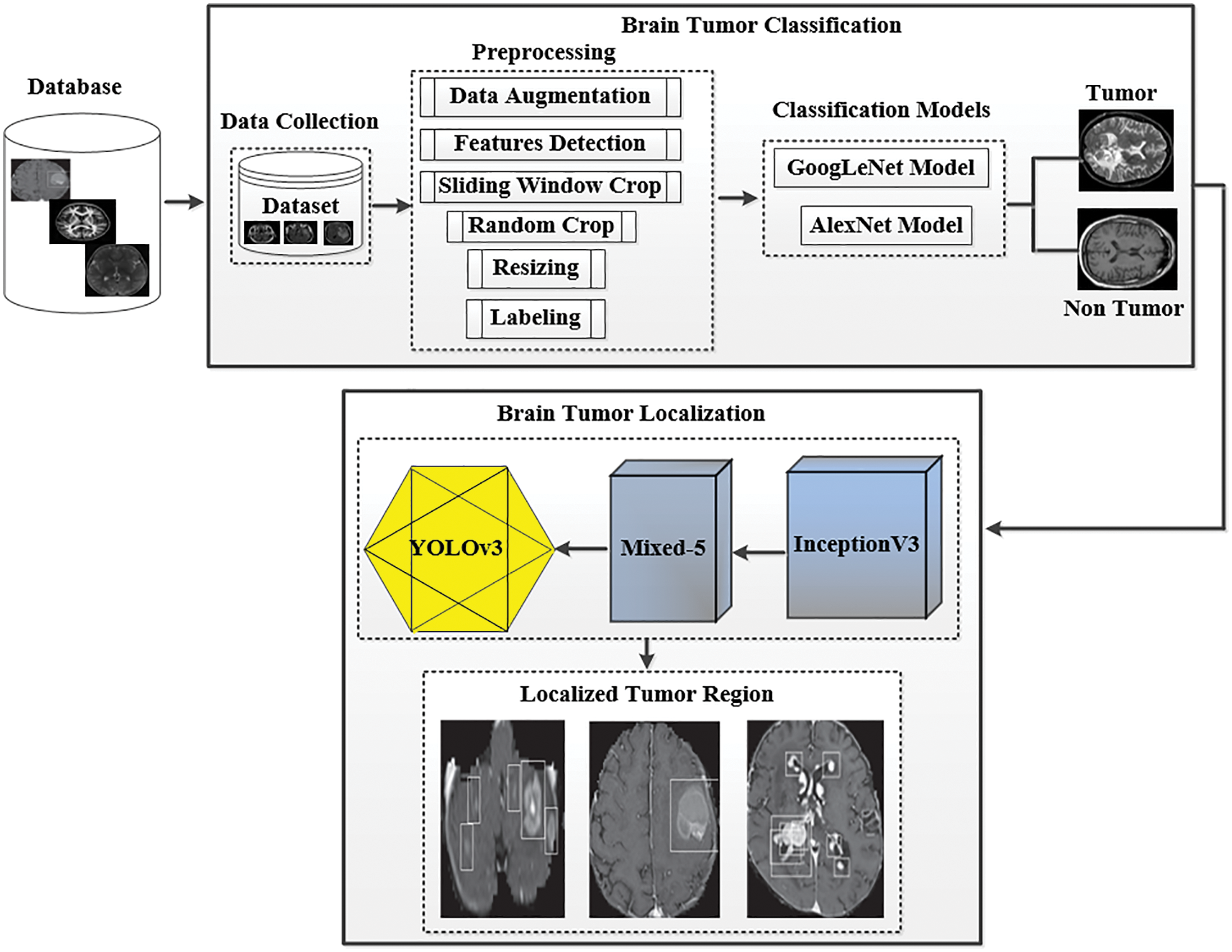
Figure 1: The proposed framework of tumor classification and localization
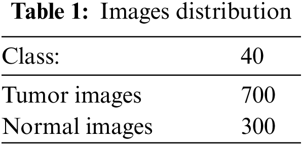
The patient's data utilized in this paper were collected from a medical institution's radiology department named Rahman Medical Institute (RMI) Peshawar, KPK, Pakistan. The collected dataset was then arranged in the form of a DICOM plan for classification. The distribution of images is shown in Tab. 1. Our collected dataset has a form of each 16 pieces with the level of pixels on the separation of the value 0.3875*0.3875 millimeters. In contrast, the widths of the data pieces were calculated at 6 millimeters. The dataset consists of T1-weighted (T1w) imaging [33]; tissues with short T1 appear brighter than tissues with longer T1, T2-weighted (T2w) imaging; tissues with long T2 appear brighter (hyperintense), and likewise as Fluid-attenuated inversion recovery (FLAIR) image having a center, coronal, and sagittal view. T1 and T2 are physical tissue properties (i.e., independent of the MRI acquisition parameters). For example, the gray matter has a T1 relaxation time of 950 ms and a T2 relaxation time of 100 ms (approximately, at 1.5 Tesla). The proposed system uses BX50 (40x strengthening aspect) for catching images from the dataset. The image is put away with no standardization and shading normalization to limit the intricacy and data misfortune in the investigation.
The preprocessing steps are utilized on the DICOM's datasets to improve the image value and outcome. The MR images are generally more challenging tasks to portray or assess because of their low-intensity scale. Also, the MR images may be dropped to a low level by such artifacts uprising from diverse resources, which can be considered significant to any process. Motion, scanner-specific variations, inhomogeneity are among the key objects that are seen in MR images. Fig. 2 shows how much the identical anatomical object is deriving and utilizing the exact procedure of the scanner. In addition, Fig. 2 also describes how much intensity value across the identical organ within the same patient, i.e., the fat tissue in Fig. 2, may vary in alternative locations. It is important to apply solid and effective procedures to prepare MR images for standardization, registration, bias field correction and denoises.
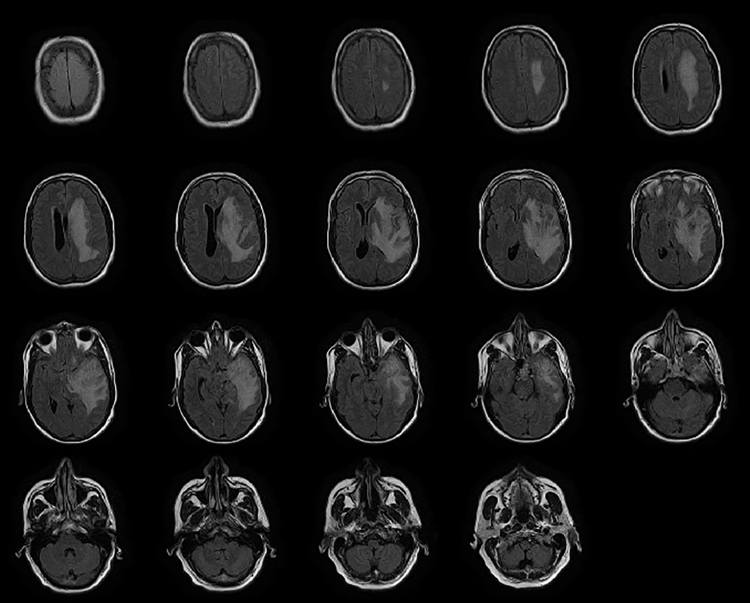
Figure 2: Northwest general hospital brain DICOM image dataset
Data Augmentation: Data augmentation is an automatic way to boost the number of different images use to train deep learning algorithms. In this work, the mathematical change of DICOM images by altering the position of the pixels has been utilized on the dataset. Several types of mathematical changes are applied to our newly created dataset. These changes include rotation by utilizing distinctive points, translation by the arbitrary move, true/bogus reversing, arbitrary point's distribution, extending with the arbitrary elasticity aspect from “1.3” to “1/1.3”. The rotation is used without considering image dimensions as the image sizes are affected, which are later adjusted by the neural network but rotating it at right angles preserves the image size. The translation involves the movement of the brain tumor images along the X and Y axis, and this method is useful because the brain tumor can be located anywhere inside the images, thereby forcing the neural network to train more effectively, i.e., looking for the object inside the image in all directions. Similarly, other standard data augmentation techniques are applied to evolve the data size intelligently because deep neural networks are highly dependent on the size of the data; the huge is the size of the data, the better a model gets trained and vice versa. Our dataset contains 1000 images. After data augmentation, we have three possible ways for our images: random rotation, random noise, and horizontal flip. With data augmentation script, we have generated 1000 new images.
Features Detection: The second step of pre-processing is to incorporate feature ID. Feature ID is utilized to extract the information gained from images and find the accurate pixel of the images that can fit in the window size.
Sliding Window Crop: This approach is used to crop the size of the picture for better classification and segregation. The approach makes it easy to resize the image; it crops the image according to the window size in which it can be kept and fit perfectly by both height and width. In addition, it also makes it easy the process of transfer learning and feature extraction because only the target area of the image will be left for processing. When this procedure is performed, it will be marked as the window size N of the slide size. Then, this will become M(N*N) on the images, equal to 00.05 N. The layers over diverse harvests are utilized to secure the data structure from any kind of damage.
Unpredictable Crop: It is utilized to handle overgrowing by setting the irregular yield size N*N. It does not utilize the managing of the sliding window.
Resizing: This step resizes the image to best fit in window sliding. Fig. 3 illustrates the resized image from one format to another, with the notation of x, y and z, which portrays the resizing value by 224*224.
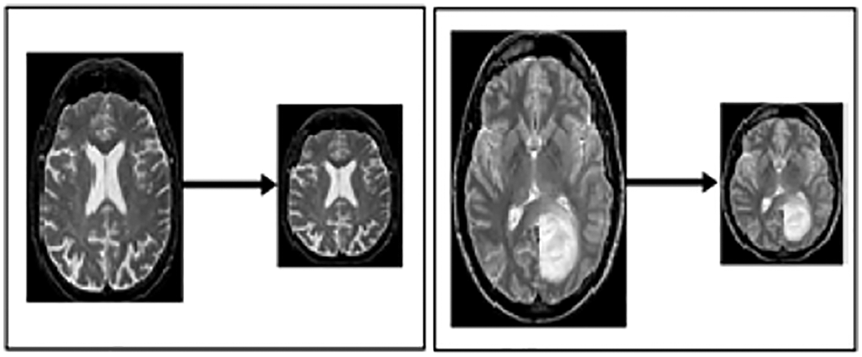
Figure 3: Resized MRI image
Labeling of Class: This technique assigned a label to each class with different numbers or notation (Class 0 and 1). Class 0 denotes that there is no tumor detected in images (called normal images). While class 1 illustrates that a tumor is detected in images (tumor cerebrum images) called Abnormal.
3.3 Image Classification Using Googlenet Model
We used the GooLeNet model is used for tumor classification. This model is utilized to handle uncommon manifestations of the beginning underlying model. A more extensive and more profound beginning link was utilized, which has somewhat bad value, yet it increases the outcomes when added all things. For demonstrational purposes, the exceptionally successful GoogLeNet model is described in Fig. 4.
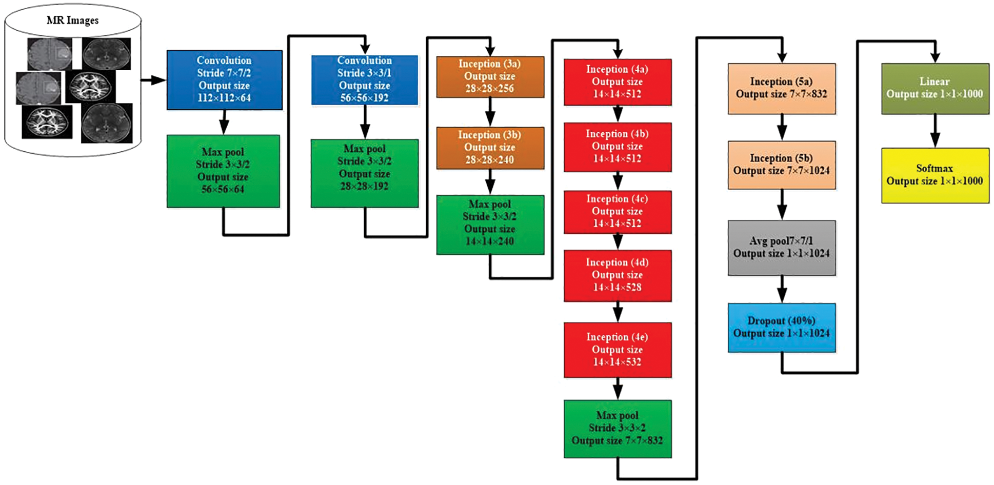
Figure 4: GoogLeNet model for image classification
The comparable methodology arranged with diverse inspecting approaches has been utilized. In these approaches, there has been undertaken six deep learning approach models from seven models. The size and the pixels of each image have taken in the range of values 0224*0224. Here, the concept of Red Green Blue (RGB) is utilized. In this scenario, the channels with the simple values of 03*03 are used for the dimension and the values of 05*05 for the declines. However, the values of 01*01 are used before the values of 03*03 and 05*05 of the convolutions. The number of 01*01diverts is used to help in the projection layer and may be viably found in the dataset named [Pool Proj] segment after the layer of max-pooling. Furthermore, an amended straight activation function is used on the whole projection and decline layers. The association of 27 layers is significant by the time of measuring pooling. In any case, it is single 22 layers on the off chance that we count layers just with limits. Therefore, the quantity of layers 100 with free construction hinders is utilized to advance the association. Nevertheless, the mentioned number of layers lie upon the establishment scheme recycled in AI. The classifier relies upon the use of ordinary pooling, which we have assorted utilization. Therefore, this accepts the current approach accordingly to utilize an extra immediate layer. This permits the association to align and changing viably for novel name sets. Consequently, it is genuinely sensible, and no critical properties stood typical or skilled. It was seen that all 1 exactness might be upgraded to 0.6%, with the mobility from totally related layers to the pooling of average. Since in the wake of wiping out, the related layers and the failure layer is recycled essentially.
The GoogLeNet model can undergo unobtrusive CNN, which results from the inception from the value of 4-a to 4-d (modules). Whereas, in the link getting ready to stage or initial stage, the adversity classifiers are the weight of 00.3. These are then discarded at the time of derivation. By checking the associate classifier, the construction of the given additional link is discussed as follows. The channel with a mean pooling layer and the size value ranged from 05*05 & 03 phases are followed by 04*04*0528 for the value mentioned above of 4-d & 04*04*0512 of the stage 4-a.
• A 1*1 convolution with 128 channels for decline estimation and revision straight inception. It is used with input layers to ease the process of CNN.
• A connected layer with 1024 units and reviewed direct incitation.
• A failure layer with a 70% ratio of dropped yields.
• A straight layer with SoftMax incident as the classifier (expecting comparative 1000 classes as the essential classifier, in any case, disposed of at inducing time).
3.4 Data Classification Using AlexNet Model
The AlexNet is a CNN-based model for the segregation and classification of images. The architecture of AlexNet model is shown in in Fig. 5. This model contains the highest ranked 14 layers. Three of them are linked layers, seven are convolutional, and 4 are ReLU and max-pooling layers. For the activation purpose, this model has 3 active layers. The images that contain useful information are utilized to possess the size and value of having 50, 50, and 3. The width and height of these images contain a channel of 50 links. The value of the active state is to be kept by the value of 1, and the window size is to be held 3, 3 with the contrast of the padding, which takes all seven layers together. When the value of step initial is 1, and the size of the segment window is in the range of 02, then the outer area kept 4 of max-pooling layers. The normalization process is utilized at every layer directly via the loop procedure to enhance the processing speed. For reducing the burden, the term dropout of 30 is utilized in a convolution layer. The dropout of 0.5 in fully connected 2 layers is exploited to decrease the level of overhead. The fully connected layer is used for the activity of softmax.
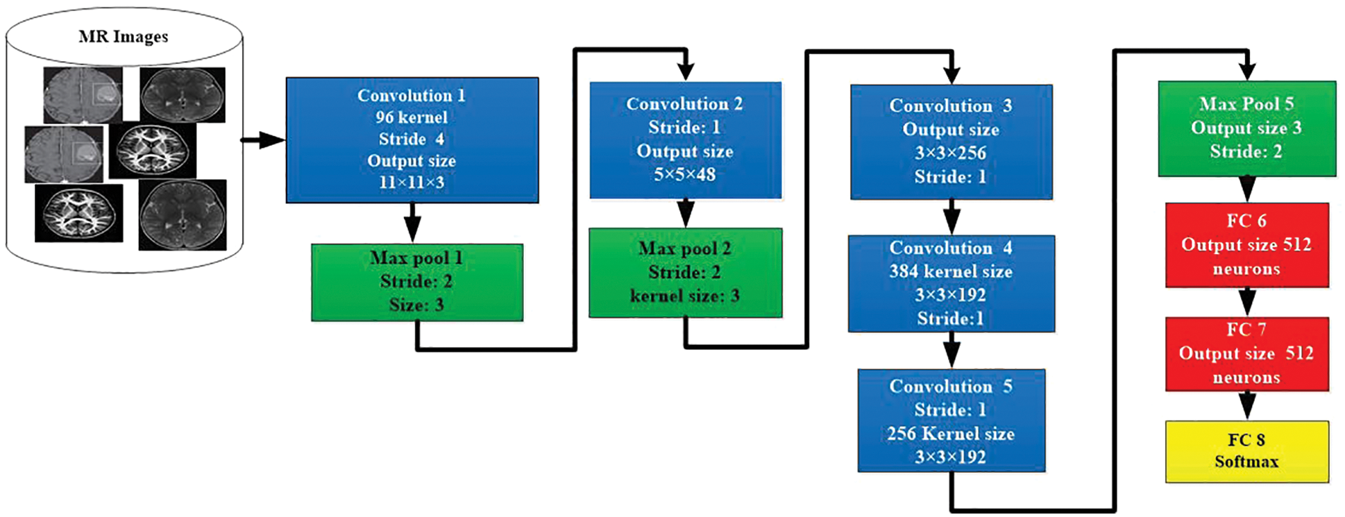
Figure 5: Architecture of AlexNet model for image classification
3.5 Tumor Localization Using YOLOv3 Model
It is important to fastly detect the exact location of a brain tumor, which helps speed up the diagnosis process. The proposed YOLOv3 model properly targets and focuses on the desired area, such as a tumor in a single image, not unlike taking the process of all the dimensions of images. The network architecture of the ‘YOLO V-3’ is shown in Fig. 6. With the proper utilization of the proposed model, the system architecture can detect tumor images effectively. The YOLOv3 estimation model can target one phase area for counting. It counts with flexibility, accuracy, authenticity and high viability by immediately handling the target plan and revelation issue. The darknet-53 is also known as the spine network of the YOLOv3 model. The up-testing network and a YOLOv3 layer are used for feedback and acknowledgment. The DarkNet-53 precisely extracts the features from the images. It is employed as the central section for overall networks. To use efficiently among the yields of diver layers, the whole number of the 5 extra layers with divers profundities are chosen. In this model, the convolutional layers are 53. They can be defined with diverse numbers in each square extra several 03*03 & 01*01 layers of brisk convolutional links. In this model, each layer has divers sub-layers called ReLU (called the rectified direct unit). The intermediate layer of the DarkNet-53 is linked with each other for certain sudden affiliation.
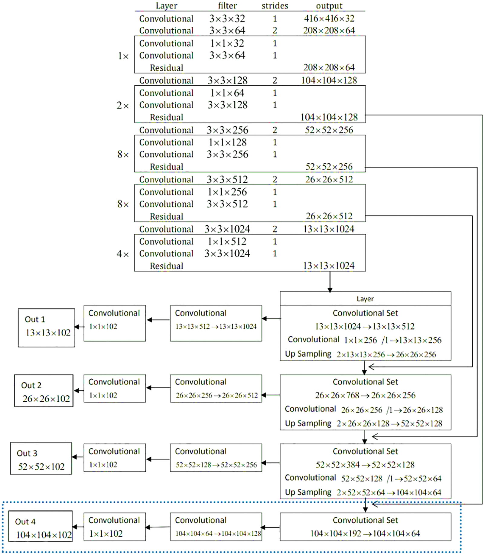
Figure 6: Network architecture of YOLOv3 model for tumor localization
To decrease the model computation tasks, the convolution 01 × 01 packs the functioned plot networks. In assessment with the previous models, the ResNet creates a more significant association, which is easy to improve, faster, with lower diverse nature, and few limits. Therefore, it can handle the issue of difficulty and burden. Darknet-53 performs five tasks for the estimation decline. In the element, the number of lines and areas of every estimation decline generated, and the significance duplicates are different from the previous. In the DarkNet-53 layout, every pixel on the component guide of diverse layers addresses the diverse values and sizes of the primary images. For instance, every pixel shown in the image addresses 124*124*128 and size 04*04 with the primary value 0416*0416 of images. With this terminology, at the exact timing, every pixel in the image is the value of 013*013*01023, which are the addresses with the limited size of 032*032 of the primary values 0416*0416 images. Therefore, the model YOLOv3 chooses values of the image are 052*052*0256, and the other values are 026*026*0512 with 013*013*01024. In this regard, the 03 component layers for the evaluation and extraction of the feature may not be changed much. It means there will not be much diversity of unique sizes. Due to different approaches, every planning image has an unmistakable size and different objectives. ‘YOLOv3’ changes the size of an image to 0416 before further usage. It is developed to refine the imaginative images and diminish with pressure planning the revelation focal point of a little size. For execution, if the element yield by Darknet-53 is picked, the feature information of little size will be last. Thus, we should add a modest layer feature with respect to the part position-subject of the main YOLOv3 layer to improve the exactness of target disclosure.
The dataset utilized in this work is discussed in Subsection 3.1. The data preprocessing modules are explained in Subsection 3.2. In this section, the performance of the abovementioned models is evaluated, and the results are discussed.
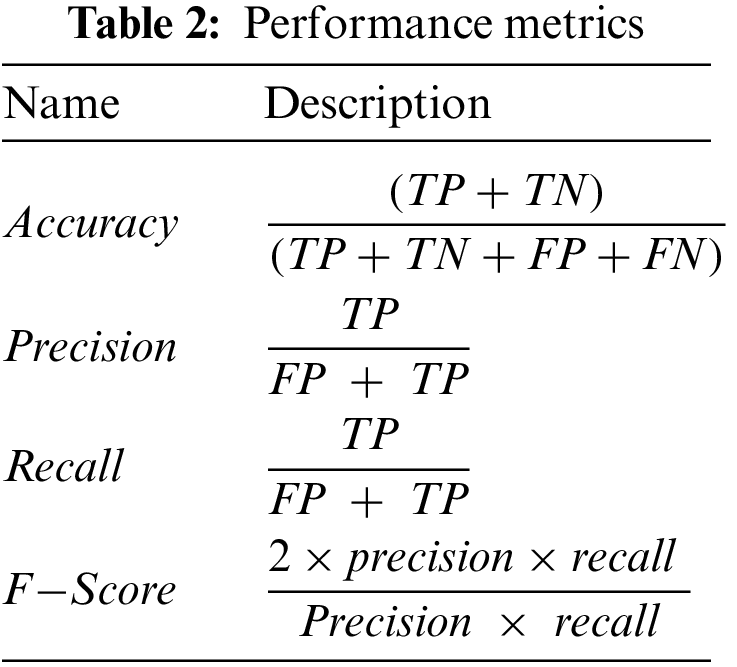
The proposed models are evaluated using two main matrices: loss and accuracy for training and validation data. In addition, we also employed different performance metrics to verify the effectiveness of the models mentioned above, as shown in Tab. 2. The data is divided into 70% and 30% for training and testing purposes, respectively. We used open-source Python libraries for algorithm implementation, including Keras with backend Tensor Flow API and Numpy running on Windows 10 Pro operating system, installed over intel core M3 CPUs, and equipped with 8GB of RAM. In this study, we utilized three CNN models, including AlexNet, GoogLeNet, and YOLOv3. The proposed technique based on CNN is a very genuine learning model for feature extraction over a high dimension space.
4.2 Performance Evaluation of GoogLeNet Model
Tab. 3 presents the training parameters of the GoogLeNet model. We have applied one max-pooling and two convolutional layers to reduce the overfitting problem and improve the classification accuracy of tumor images.
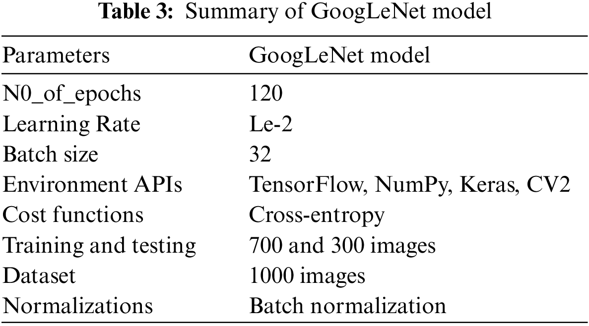
Fig. 7 presents the accuracy and loss of the proposed GoogLeNet model based on a training dataset for brain tumor classification. Epoch is the number of iterations of training data passed to the CNN model for tuning the cost function parameters.
In the GoogLeNet model, weight is changed at each epoch to produce different values of loss and accuracy. The initial accuracy at the training stage was 0.6630, which is increased to 0.9768 in the last epoch. However, the loss for the first epoch was 2. 1053, which is decreased to 0.2412 in the last epoch. These results show that the accuracy and loss of the proposed model are largely increased and decreased based on the training dataset, respectively. In the second experiment, we have utilized a testing dataset to evaluate the performance of the GoogLeNet model in terms of brain tumor classification. Fig. 8 shows the accuracy and loss of the GoogLeNet model based on the testing dataset. As shown in Fig. 8, the accuracy for the first epoch is 0.8377, which is increased to 0.9241 on epoch 120. Whereas the loss of this model on the first epoch is 1.2723, which is slightly decreased to 1.2172. However, the loss of this is largely decreased to 0.7018 on epoch 115. The results in Figs. 7 and 8 show that the GoogLeNet model can perform well for brain tumor classification.
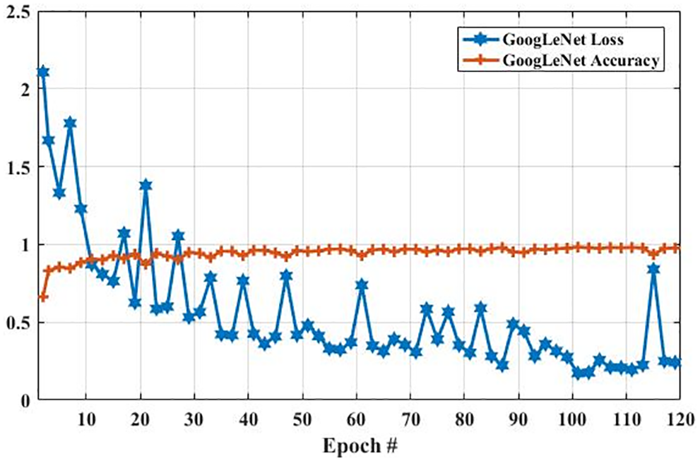
Figure 7: The GoogLeNet performance is based on the training dataset
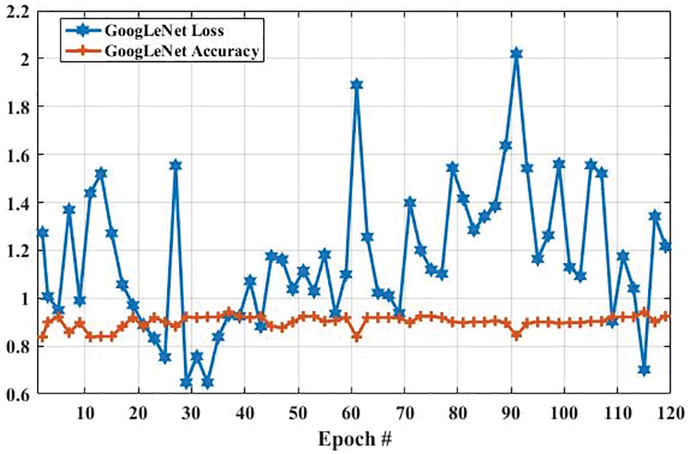
Figure 8: The GoogLeNet performance is based on a testing dataset
Fig. 9 compares the accuracy and loss of the GoogLeNet model based on the training and testing dataset. In Fig. 9a, the accuracy of the proposed model using the training dataset was 0.6630 at the first epoch, which is largely increased to 0.9768 on epoch 120. In addition, the accuracy using the testing dataset is increased from 0.85 to 0.90. Furthermore, Fig. 9b shows the comparison of GoogLeNet loss based on the training and testing dataset. As it can be clearly seen, the loss on the first epoch is 2.1053, which is largely declined to 0.5 when the number of an epoch is 120. Also, the loss of the proposed model based on the testing dataset is slightly decreased from 1.2723 to 1.2172 when the epoch is increased from 1 to 120.
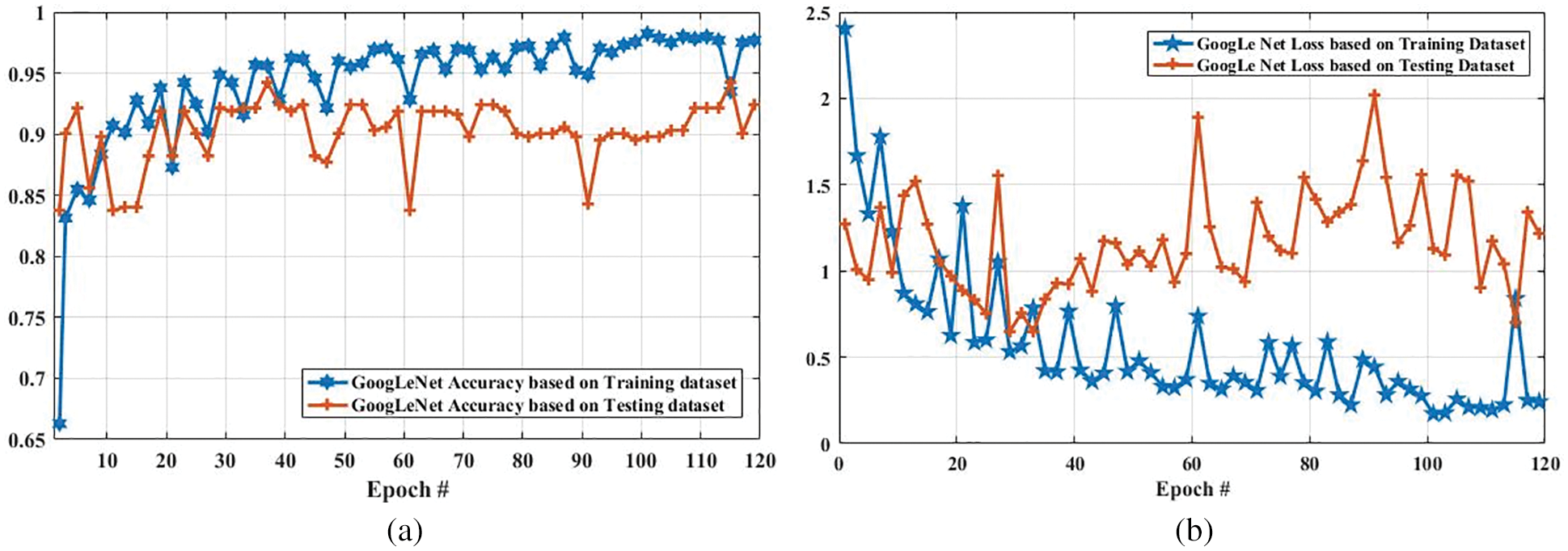
Figure 9: Accuracy and loss comparison of GoogLeNet model based on training and testing dataset. (a) Depicts the accuracy of GoogLeNet model based on training and testing dataset, and (b) illustrates the loss of GoogLeNet model based on training and testing dataset
4.3 Performance Evaluation of AlexNet Model
Here, we present the results of MR images classification using the AlexNet model. The same parameters are utilized for both AlexNet and GoogLeNet models, which are presented in Tab. 3. However, additional layers are added to reduce the overfitting problem; one max-pooling layer and two convolutional layers into the AlexNet model. We trained the AlexNet model and obtained the accuracy and loss per epoch. The accuracy of brain tumor classification per loss is shown in Fig. 10. On the first epoch, the accuracy of this model using the training dataset was 0.5510. However, when the number of epochs increases, the accuracy improves and reaches 0.8392 (on the last epoch). Furthermore, the loss of this model for the training dataset was largely decreased from 0.8512 to 0.2802 when the number of an epoch is increased. In machine learning models, epoch labels the number of passes in the entire training dataset. In this model, different weights were assigned at every epoch to gain the changed value of loss and their accuracy. The accuracy and loss of this model using testing dataset were also identified to understand it more clearly before comparing it with other models. Fig. 11 shows the accuracy per loss of the AlexNet-based brain tumor classification using a testing dataset. On the first epoch, the testing accuracy of this model was 0.6780. However, it is slightly decreased with the increasing number of an epoch. The accuracy on the last epoch is 0.6414, as shown in Fig. 11. On the other hand, the loss of this model using the testing dataset was 3.742 on the first epoch, but it gradually increased up to 5.721 till the last epoch. These results show that the AlexNet model cannot perform well in case MR images classification for tumor detection.
Fig. 12 shows the accuracy and loss of the AlexNet model based on the training and testing dataset. In Fig. 12a, with the increased epoch, the accuracy of the AlexNet model based on the training dataset was largely increased (from 0.5510 to 0.8392), whereas the accuracy based on the testing dataset was slightly decreased from 0.6780 to 0.6414. The loss of this model based on both training and the testing dataset is also compared, and the results are shown in Fig. 12b. As it can be seen that the loss of this model based on the training dataset was increased. However, it was decreased based on the testing dataset.
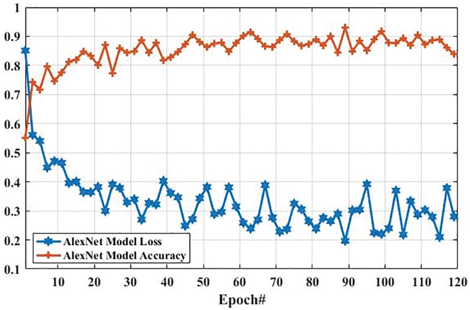
Figure 10: The AlexNet performance is based on the training dataset
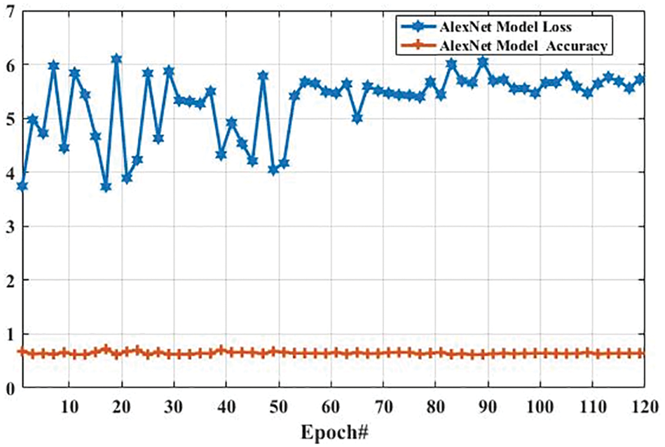
Figure 11: The AlexNet performance is based on the testing dataset
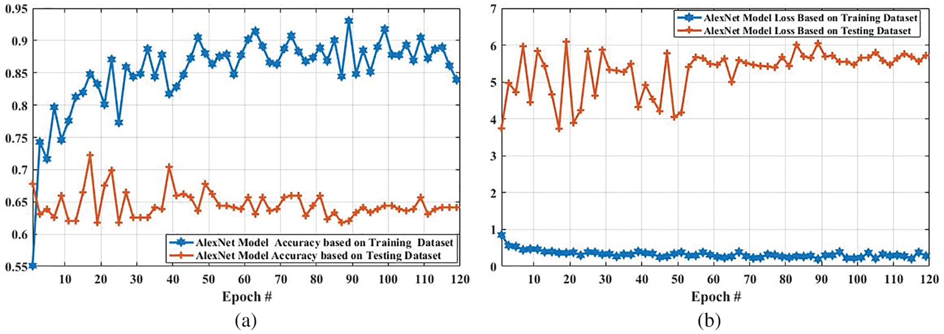
Figure 12: Accuracy and loss comparison of AlexNet model based on training and testing dataset. (a) Depicts the accuracy comparison of AlexNet model based on training and testing dataset, and (b) presents the loss comparison of AlexNet model based on training and testing dataset
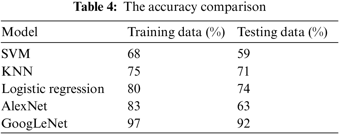
Tab. 4 presents the accuracy of tumor classification of both Google Net and AlexNet models. In this table, it is observed that the proposed model achieved 97% and 92% accuracy based on training and testing data, respectively. However, the AlexNet model achieved 83% and 63% accuracy using training and testing data, respectively. In addition, the results of other classifiers such as SVM, k-nearest neighbors (KNN), and logistic regression are also achieved in order to compare the proposed model performance with them. SVM, logistic regression, KNN are applied with parameter quadratic kernel function, ridge estimator, and a Euclidean distance function with k = 5, respectively. The SVM, KNN, and logistic regression obtained an accuracy of 68%, 75%, and 80% using training data while using testing data, the accuracy of 59%, 71%, and 74, respectively. It is observed that the accuracy of the proposed GoogLeNet model based on training and testing datasets is enhanced compared with AlexNet model and traditional existing classifiers. This result shows that the proposed model can improve its performance when the number of the epoch is increased. This result also indicates that the proposed model can perform better than the AlexNet model in tumor classification.
4.4 Performance Evaluation of YOLOv3 Model
Fig. 13 shows the accuracy and loss of YOLOv3-based tumor localization using the training dataset. The accuracy of the YOLOv3 model at the first epoch was 0.729, which is increased to 0.819 in the last epoch. Whereas the loss at the first epoch was 0.755 using training data, which is largely decreased to 0.204 in the last epoch. Similarly, the accuracy and loss of the YOLOv3 model using the testing dataset are shown in Fig. 14. As shown in Fig. 14, the loss decreases from 3.48 to 0.627, whereas the accuracy increases from 0.478 to 0.943.
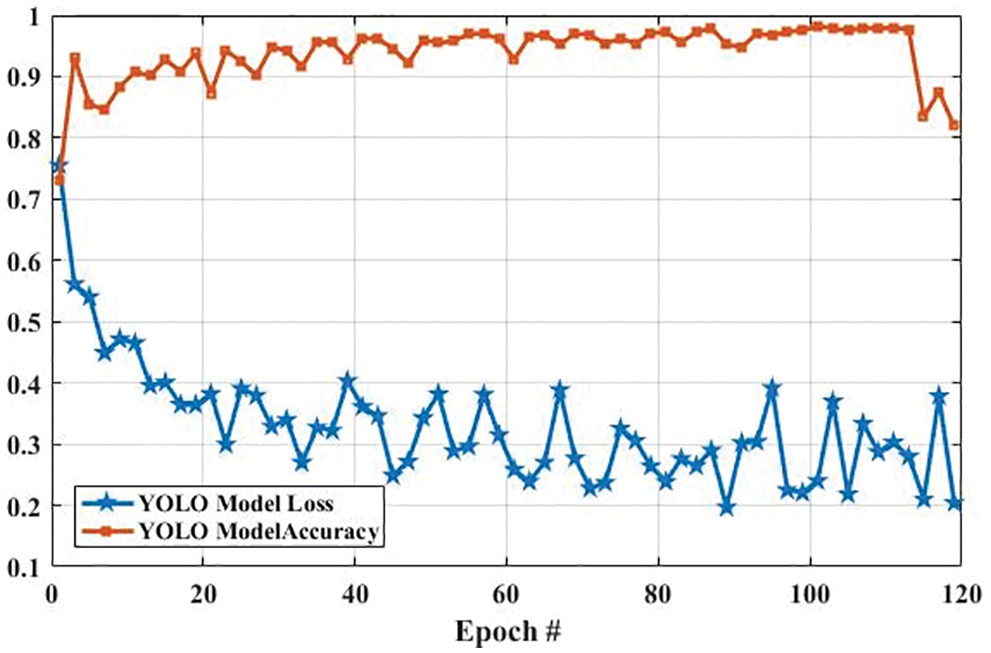
Figure 13: The YOLO model performance is based on training data
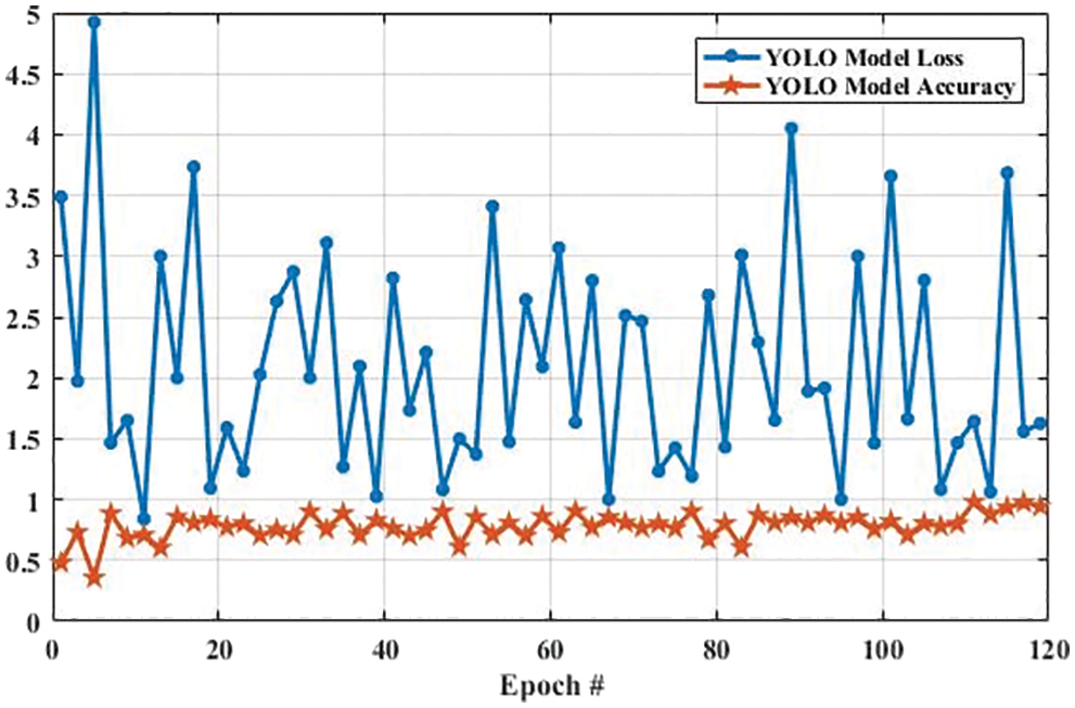
Figure 14: The YOLO model performance is based on testing data
The accuracy and loss of the YOLOv3 model based on the training and testing dataset are also compared, and the results are shown in Fig. 15. Fig. 15a shows that the accuracy of the YOLOv3 model is increased from 0.729 to 0.819 and 0.478 to 0.943 using the training and testing dataset, respectively. However, the loss of the YOLOv3 model is decreased from 0.755 to 0.204 and 3.488 to 0.627 using training and testing datasets, respectively, as shown in Fig. 15b. Furthermore, the results of tumor localization in images using the YOLOv3 model are shown in Fig. 16.
The proposed GoogLeNet model performed well in terms of accuracy. The proposed algorithm based on CNN features is the most feasible learning model for feature selection over a higher dimension space. The experimental results show that CNN (Features + Classification) performs better in feature selection, optimization, and tumor classification. Hence, the proposed method improves the classification accuracy by minimal optimization of the feature sets.
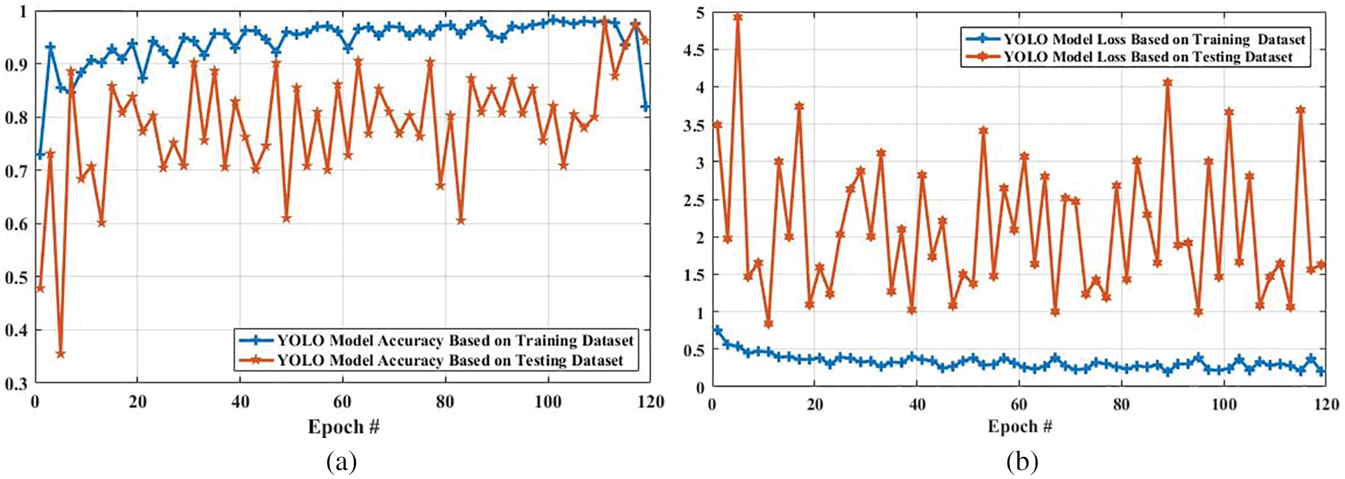
Figure 15: Accuracy and loss comparison of YOLO model based on training and testing dataset. (a) Shows the accuracy comparison of YOLO model based on training and testing dataset, and (b) presents the loss comparison of YOLO model based on training and testing dataset
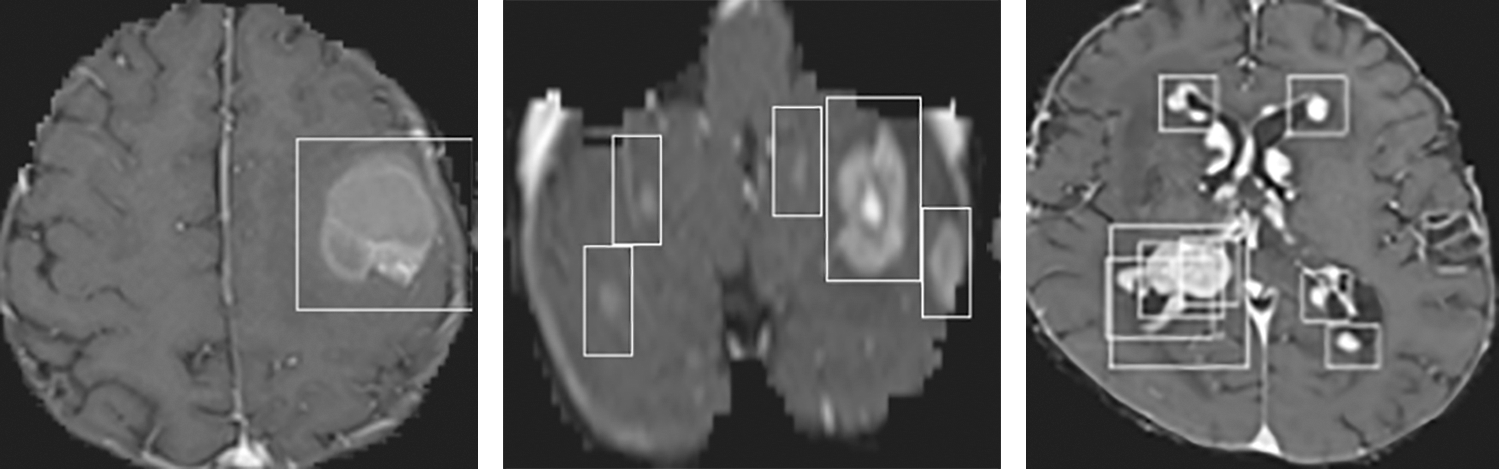
Figure 16: Tumor Localization in images using the YOLOv3 model
In this paper, an automatic system of tumor classification and detection is proposed using deep learning models. Various methods are applied to efficiently classify the tumor in MR images. Both the GoogLeNet and AlexNet models are trained with different parameters. The parameters in these models are tuned to select the best parameters to achieve higher accuracy and time efficiency. The proposed system can precisely filter the data, extract the features, classify the tumor images, and localize the tumor in images. The proposed system achieved an accuracy of 97%, while the AlexNet model obtained 83%. Compared to the AlexNet model, the proposed model shows more precise results in simulations with very few losses. Therefore, it is concluded that the proposed GoogLeNet model is an appropriate method for tumor image classification and the YOLOv3 model for tumor localization in MR images. In future work, novel methods for features extraction will be examined to know the efficiency of the proposed method. In addition, various batch sizes and a number of epochs will be tested in the proposed model, and then the results of the model will be compared with other classifiers.
Funding Statement: This work is supported by Institute for Information & communications Technology Promotion (IITP) grant funded by the Korea government (MSIT) (No. 2016-0-00145, Smart Summary Report Generation from Big Data Related to a Topic). This research work was also supported by the Research Incentive Grant R20129 of Zayed University, UAE.
Conflicts of Interest: The authors declared that they have no conflicts of interest.
1. I. Despotović, B. Goossens and W. Philips, “MRI segmentation of the human brain: Challenges, methods, and applications,” Computational and Mathematical Methods in Medicine, vol. 2015, pp. 1–24, 2015. [Google Scholar]
2. S. D. S. Al-Shaikhli, M. Y. Yang and B. Rosenhahn, “Brain tumor classification using sparse coding and dictionary learning,” in 2014 IEEE Int. Conf. on Image Processing (ICIP), Paris, France, pp. 2774–2778, 2014. [Google Scholar]
3. L. Yi and G. Zhijun, “A review of segmentation method for MR image,” in 2010 Int. Conf. on Image Analysis and Signal Processing, Zhejiang, China, pp. 351–357, 2010. [Google Scholar]
4. D. Ray, D. D. Majumder and A. Das, “Noise reduction and image enhancement of MRI using adaptive multiscale data condensation,” in 2012 1st Int. Conf. on Recent Advances in Information Technology (RAIT), Dhanbad, India, pp. 107–113, 2012. [Google Scholar]
5. S. M. A. Sharif, R. A. Naqvi and M. Biswas, “Learning medical image denoising with deep dynamic residual attention network,” Mathematics, vol. 8, pp. 2192, 2020. [Google Scholar]
6. R. Kinnard, “Why is grey matter outside of the brain, and inside the spinal cord?,” in Quora ed, 2017. [Google Scholar]
7. P. Natarajan, N. Krishnan, N. S. Kenkre, S. Nancy and B. P. Singh, “Tumor detection using threshold operation in MRI brain images,” in 2012 IEEE Int. Conf. on Computational Intelligence and Computing Research, Coimbatore, India, pp. 1–4, 2012. [Google Scholar]
8. J. Amin, M. Sharif, M. Raza, T. Saba and A. Rehman, “Brain tumor classification: Feature fusion,” in 2019 Int. Conf. on Computer and Information Sciences (ICCIS), Sakaka, Saudi Arabia, pp. 1–6, 2019. [Google Scholar]
9. Z. Ullah, M. U. Farooq, S. -H. Lee and D. An, “A hybrid image enhancement based brain MRI images classification technique,” Medical Hypotheses, vol. 143, pp. 109922, 2020. [Google Scholar]
10. M. K. Abd-Ellah, A. I. Awad, A. A. Khalaf and H. F. Hamed, “Two-phase multi-model automatic brain tumour diagnosis system from magnetic resonance images using convolutional neural networks,” EURASIP Journal on Image and Video Processing, vol. 2018, pp. 1–10, 2018. [Google Scholar]
11. W. Deng, W. Xiao, H. Deng and J. Liu, “MRI brain tumor segmentation with region growing method based on the gradients and variances along and inside of the boundary curve,” in 2010 3rd Int. Conf. on Biomedical Engineering and Informatics, Yantia, China, pp. 393–396, 2010. [Google Scholar]
12. M. Toğaçar, B. Ergen and Z. Cömert, “BrainMRNet: Brain tumor detection using magnetic resonance images with a novel convolutional neural network model,” Medical Hypotheses, vol. 134, pp. 109531, 2020. [Google Scholar]
13. W. Wu, D. Li, J. Du, X. Gao, W. Gu et al., “An intelligent diagnosis method of brain MRI tumor segmentation using deep convolutional neural network and SVM algorithm,” in Computational and Mathematical Methods in Medicine, vol. 2020, Hindawi, 2020. [Google Scholar]
14. A. Rosset, L. Spadola and O. Ratib, “OsiriX: An open-source software for navigating in multidimensional DICOM images,” Journal of Digital Imaging, vol. 17, pp. 205–216, 2004. [Google Scholar]
15. S. Deepak and P. Ameer, “Retrieval of brain MRI with tumor using contrastive loss based similarity on googLeNet encodings,” Computers in Biology and Medicine, vol. 125, pp. 103993, 2020. [Google Scholar]
16. A. Rehman, M. A. Khan, T. Saba, Z. Mehmood, U. Tariq et al., “Microscopic brain tumor detection and classification using 3D CNN and feature selection architecture,” Microscopy Research and Technique, vol. 84, pp. 133–149, 2021. [Google Scholar]
17. P. A. Yushkevich, J. Piven, H. C. Hazlett, R. G. Smith, S. Ho et al., “User-guided 3D active contour segmentation of anatomical structures: Significantly improved efficiency and reliability,” Neuroimage, vol. 31, pp. 1116–1128, 2006. [Google Scholar]
18. H. Khotanlou, O. Colliot, J. Atif and I. Bloch, “3D brain tumor segmentation in MRI using fuzzy classification, symmetry analysis and spatially constrained deformable models,” Fuzzy Sets and Systems, vol. 160, pp. 1457–1473, 2009. [Google Scholar]
19. E. I. Zacharaki, S. Wang, S. Chawla, D. S. Yoo, R. Wolf et al., “Classification of brain tumor type and grade using MRI texture and shape in a machine learning scheme,” Magnetic Resonance in Medicine: An Official Journal of the International Society for Magnetic Resonance in Medicine, vol. 62, pp. 1609–1618, 2009. [Google Scholar]
20. A. O. Algohary, A. M. El-Bialy, A. H. Kandil and N. F. Osman, “Improved segmentation technique to detect cardiac infarction in MRI C-SENC images,” in 2010 5th Cairo Int. Biomedical Engineering Conf., Cairo, Egypt, pp. 21–24, 2010. [Google Scholar]
21. D. M. Joshi, N. Rana and V. Misra, “Classification of brain cancer using artificial neural network,” in 2010 2nd Int. Conf. on Electronic Computer Technology, Kuala Lumpur, Malaysia, pp. 112–116, 2010. [Google Scholar]
22. J. Juan-Albarracín, E. Fuster-Garcia, J. V. Manjon, M. Robles, F. Aparici et al., “Automated glioblastoma segmentation based on a multiparametric structured unsupervised classification,” PLoS One, vol. 10, pp. e0125143, 2015. [Google Scholar]
23. J. Cheng, W. Huang, S. Cao, R. Yang, W. Yang et al., “Enhanced performance of brain tumor classification via tumor region augmentation and partition,” PLoS One, vol. 10, pp. e0140381, 2015. [Google Scholar]
24. A. Veeramuthu, S. Meenakshi and V. P. Darsini, “Brain image classification using learning machine approach and brain structure analysis,” Procedia Computer Science, vol. 50, pp. 388–394, 2015. [Google Scholar]
25. P. A. Yushkevich, Y. Gao and G. Gerig, “ITK-SNAP: An interactive tool for semi-automatic segmentation of multi-modality biomedical images,” in 2016 38th Annual Int. Conf. of the IEEE Engineering in Medicine and Biology Society (EMBC), Orlando, FL, USA, pp. 3342–3345, 2016. [Google Scholar]
26. T. Araújo, G. Aresta, E. Castro, J. Rouco, P. Aguiar et al., “Classification of breast cancer histology images using convolutional neural networks,” PLoS One, vol. 12, pp. e0177544, 2017. [Google Scholar]
27. J. Kang, Z. Ullah and J. Gwak, “MRI-Based brain tumor classification using ensemble of deep features and machine learning classifiers,” Sensors, vol. 21, pp. 2222, 2021. [Google Scholar]
28. I. Abd El Kader, G. Xu, Z. Shuai, S. Saminu, I. Javaid et al., “Differential deep convolutional neural network model for brain tumor classification,” Brain Sciences, vol. 11, pp. 352, 2021. [Google Scholar]
29. Z. N. K. Swati, Q. Zhao, M. Kabir, F. Ali, Z. Ali et al., “Brain tumor classification for MR images using transfer learning and fine-tuning,” Computerized Medical Imaging and Graphics, vol. 75, pp. 34–46, 2019. [Google Scholar]
30. O. Sevli, “Performance comparison of different Pre-trained deep learning models in classifying brain MRI images,” Acta Infologica, vol. 5, pp. 141–154, 2021. [Google Scholar]
31. M. I. Sharif, J. P. Li, J. Amin and A. Sharif, “An improved framework for brain tumor analysis using MRI based on YOLOv2 and convolutional neural network,” Complex & Intelligent Systems, vol. 7, pp. 1–14, 2021. [Google Scholar]
32. A. Çinar and M. Yildirim, “Detection of tumors on brain MRI images using the hybrid convolutional neural network architecture,” Medical Hypotheses, vol. 139, pp. 109684, 2020. [Google Scholar]
33. R. A. Naqvi, D. Hussain and W. -K. Loh, “Artificial intelligence-based semantic segmentation of ocular regions for biometrics and healthcare applications,” Computers, Materials & Continua, vol. 66, no. 1, pp. 715–732, 2021. [Google Scholar]
 | This work is licensed under a Creative Commons Attribution 4.0 International License, which permits unrestricted use, distribution, and reproduction in any medium, provided the original work is properly cited. |