Computers, Materials & Continua DOI:10.32604/cmc.2022.023693
Article

Unstructured Oncological Image Cluster Identification Using Improved Unsupervised Clustering Techniques

S. Sreedhar Kumar1, Syed Thouheed Ahmed2,*, Qin Xin3, S. Sandeep4, M. Madheswaran5 and Syed Muzamil Basha2

1Dr. T. Thimmaiah Institute of Technology, VTU, KGF, Karnataka, India
2School of Computing & Information Technology, REVA University, Bengaluru, India
3Faculty of Science and Technology, University of the Faroe Islands, Faroe Islands, Denmark
4K S School of Engineering, Bengaluru, India
5Muthayammal Engineering College, Rasipuram, Tamil Nadu, India
*Corresponding Author: Syed Thouheed Ahmed. Email: syed.edu.in@gmail.com
Received: 17 September 2021; Accepted: 10 December 2021

Abstract: This paper presents, a new approach of Medical Image Pixels Clustering (MIPC), aims to trace the dissimilar patterns over the Magnetic Resonance (MR) image through the process of automatically identify the appropriate number of distinct clusters based on different improved unsupervised clustering schemes for enrichment, pattern predication and deeper investigation. The proposed MIPC consists of two stages: clustering and validation. In the clustering stage, the MIPC automatically identifies the distinct number of dissimilar clusters over the gray scale MR image based on three different improved unsupervised clustering schemes likely improved Limited Agglomerative Clustering (iLIAC), Dynamic Automatic Agglomerative Clustering (DAAC) and Optimum N-Means (ONM). In the second stage, the performance of MIPC approach is estimated by measuring Intra intimacy and Intra contrast of each individual cluster in the result of MR image based on proposed validation method namely Shreekum Intra Cluster Measure (SICM). Experimental results show that the MIPC approach is better suited for automatic identification of highly relative dissimilar clusters over the MR cancer images with higher Intra closeness and lower Intra contrast based on improved unsupervised clustering schemes.

Keywords: Magnetic resonance image; unsupervised clustering scheme; intra intimacy; intra contrast; iLIAC; shreekum intra cluster measure; medical image clustering

1  Introduction

Cluster based image segmentation is a significant and mathematical process in the MR image analysis system for deeper investigation, enhancement, tumor predication and pattern identification. Generally, it is defined as a process of dividing MR image pixels into different numbers of dissimilar sub regions based on pixel intensity similarity [1]. The goal of cluster based image separation is to simplify or change the representation of an image into a version that is more meaningful and easier to investigate and identify. Recently, many of the researchers have been reported in [2], the cluster based segmentation process is applied in many medicine related application likely medical image segmentation, tumor or cancer predication, medical image enhancement, medical image compression, pattern identification, medical image classification and medical image retrieval. The result of the cluster based medical image separation is a finite number of dissimilar groups that jointly concealments the complete medical image and the quality of the clustering result depend on the superiority of the medical image quality. The major problem in the existing clustering schemes such as semi-supervised and unsupervised methods [3] is that to predetermine the appropriate number of clusters in the unstructured MR image pixel set and respectively the clustering quality is based on predetermined number of clusters. To overcome these issues, in this paper a new clustering technique called Medical Image Pixels Clustering, it intentions to automatically separate finite number of dissimilar patterns in the MR image based on different improved unsupervised clustering schemes without predetermined knowledge for deeper investigation, enhancement, pattern predication and analysis.

2  Literature Reviews

Several methods are available for cluster based MR image segmentation process including k-means, fuzzy C-means, neural network, fuzzy clustering and hierarchical clustering methods reported in [4–7]. The k-means technique is a semi-supervised partitioned clustering technique and is an iterative procedure that directly decomposes the MR image pixel set into many dissimilar clusters or regions by minimizing the criterion function (e.g., sum-of-square-error) [8]. Many of the authors suggested problem in the K-Means technique is that the entire segmentation result quality of MR image is based on predetermined k number of centroid pixel values. In [9], the authors Jianwei et al. have reported an improved K-Means technique MR brain image segmentation. The improved K-Means scheme is used to identify K distinct clusters over the disordered MR brain image with higher accuracy compared to existing scheme.

Another popular method called fuzzy c-means clustering (FCM) technique was reported in [10,11]. This method is suited to partition the noise-free image into a finest number of groups. Many researchers suggested that the drawback with this method is that it failed to segment images corrupted by noise or inaccurate edges. In [12] the authors Yogita et al. have reported a detail survey of fuzzy C-means (FCM) with intensity inhomogeneity correction and noise robustness. They are discussed how the FCM schemes is better suitable to identify distinct tissues such as cerebrospinal fluid, gray matter and white matter over the MR brain image. The authors Senthilkumar et al. [13] have presented a modified fuzzy C-means clustering scheme to identify the normal and abnormal tissues likely white matter, gray matter, cerebrospinal and tumor part respectively over the MRI brain image. The clustering scheme consists of pre-processing and segmentation stages. In the pre-processing stage, the authors are applied wrapping based curvelet transform over the MR brain image and removed the noise. Similarly, they are applied improved fuzzy C-Means technique [14,15] and segmented the normal and abnormal tumor cells over the MR brain image based on spatial information. In [16], the authors Jinn et al. have reported a hierarchical genetic algorithm with fuzzy learning vector quantization network to partition a multi-spectral MR brain image. The evaluation of this approach was based on a real case of a MR brain image of an individual suffering from meningioma.

The author's Chong et al. [17] have presented hybrid clustering scheme combined with morphological operations to improve the performance of MR image segmentation and reduced the non-brain tissue in the brain image. Firstly, the authors applied wiener filter and morphological operations over the MR image due to remove the non-brain tissue. Next, they are used combination of K-Means++ and kernel-based fuzzy C-Means algorithm to identify distinct tumor regions in the MR image without noise. In [18,19], the authors Kalyanapu et al. have presented a clustering scheme namely unified iterative partitioned fuzzy clustering (U-IPFC). The U-IPFC scheme uses to identify distinct tissues over the MR brain image with good accuracy. The authors in [18,19] have claimed that the U-IPFC has produced higher accuracy result compared to FCM and K-means schemes. The authors Arul et al. in [20] presented a hierarchical clustering based segmentation (HCS) scheme to identify the distinct groups in hierarchy manner over the dynamic contrast enhanced magnetic resonance (DCSMR) image pixel set. The authors claimed that the HCS scheme is acted a semi-quantitative analytical tool to discover the DCEMR images. Next, the same authors Arul et al. in [21] have extended the detailed research of MR image segmentation based on hierarchical clustering scheme. The authors have experimented HCS scheme over the Multi-parametric Magnetic Resonance Imaging (MPMRI) and identified finite number of dissimilar tissue patterns by sequence of merging process. Another author Filipovych et al. in [22] reported hierarchical clustering scheme based image segmentation and it uses to identify predetermined number of dissimilar clusters in the tree manner over the gray scale image.

3  Proposed Image Pixel Clustering Approach

This section describes detailed study of the MIPC approach of image pixels classification. The MIPC scheme consists of two stages clustering and validation. The first stage automatically identifies the distinct number of highly relative clusters over the gray scale image dataset based on three different improved unsupervised clustering schemes iLIAC, DAAC and ONM in distinct manner. The second stage, it estimates the intra cluster intimacy and intra cluster contrast over the result of clustering stage based on the proposed SICM scheme. The stages involved in the MIPC approach are illustrated in the Fig. 1 and the different stages are described in below subsections.

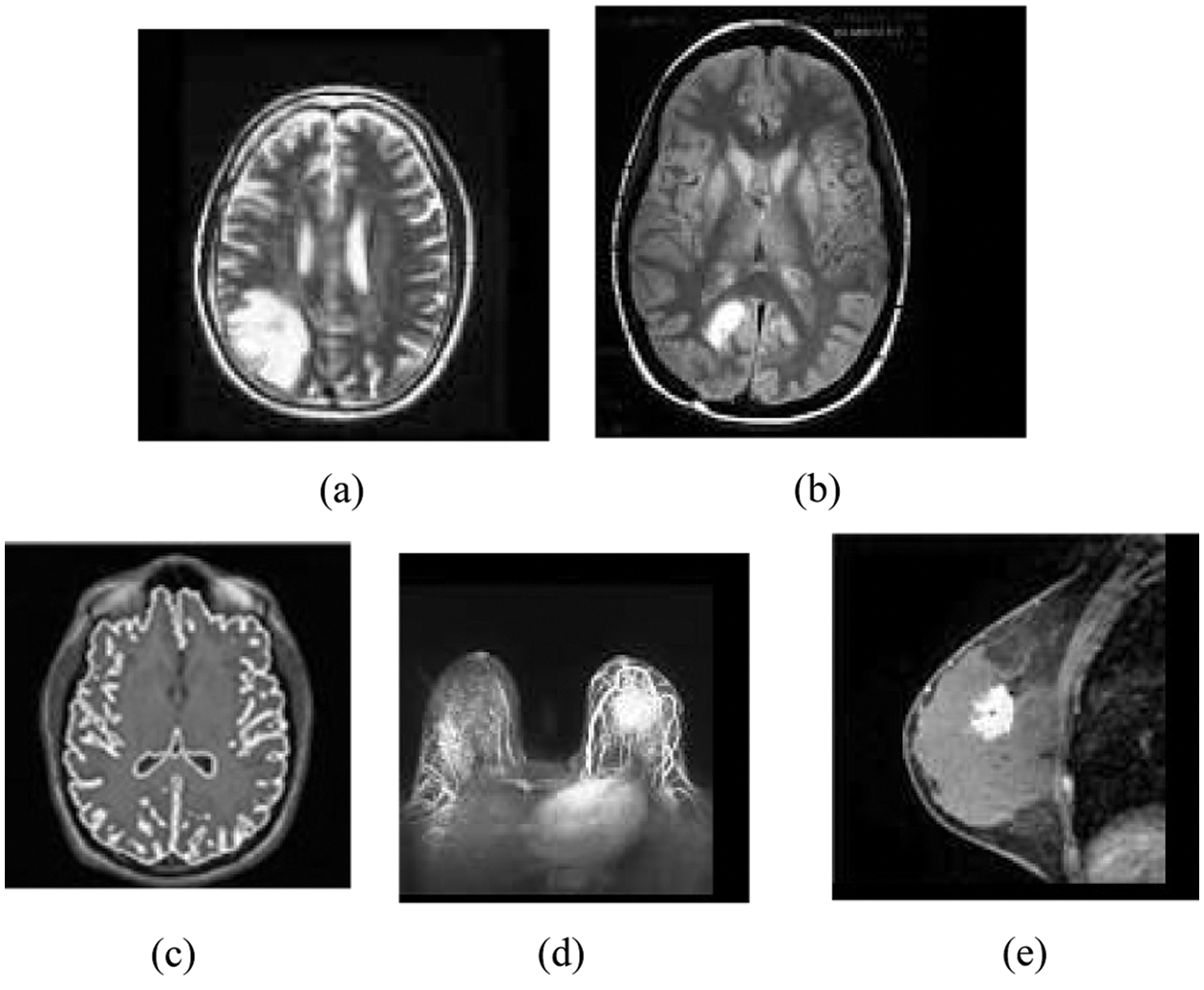
Figure 1: Original MR images: (a) Brain_1, (b) Brain_2, (c) Brain_3 (d) Breast_1 (e) Breast_2

3.1 Clustering Stage

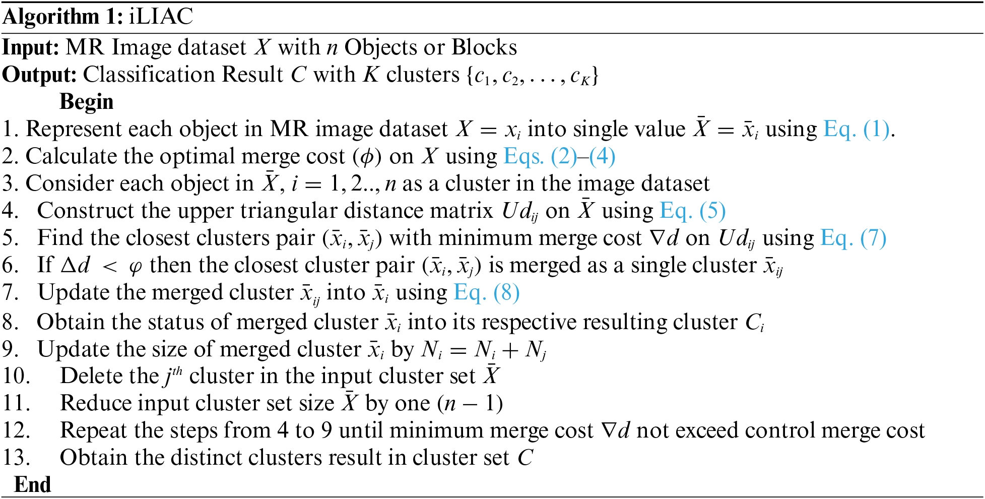
This stage automatically identifies the distinct number of dissimilar clusters on the gray scale image based on three different improved clustering schemes iLIAC [23,24], DAAC [25] and ONM [26] in separate manner. Initially, the digital gray-scale image divides into (2 * 2) sizes of non-overlapping blocks and the image contains n objects plus is defined as X=xi, xi=xij for i=1,2,…,n and j=0,1,2,…,d, where X represents the dataset of MR image with n objects or blocks, xi represents the ith object or block in dataset X, n denotes the size of MRI image dataset X, xij is the jth pixel value in ith object in dataset X and d denotes the number of pixels belongs into the each individual block in dataset X. The MIPC approach identifies distinct clusters over the image dataset X using three different improved clustering schemes iLIAC, DAAC and ONM. The clustering schemes are described below subsections.

3.2 MIPC Using iLIAC Scheme

The MIPC approach identifies distinct number of dissimilar clusters over the MRI image dataset X=xi for i=1,2,…,n based on improved agglomerative clustering iLIAC scheme [23] and it consists of three stages feature extraction, control merge cost, clustering. In the feature extraction stage, the iLIAC scheme is extracted single feature value over each individual vector or block in the MR image vector set X=xi for i=1,2,…,n with d pixels xi=xij for j=0,1,2,…,d based on statistical mean operation and is defined in the Eq. (1) as

x¯i={∑i=1n∑j=1dxijd|∀xij∈xi,∀xi∈X}(1)

where xij represents the jth pixel value in ith object that belongs in to the vector set X and d denotes the number of pixel values in ith object in X for j=1,2,…,d. Next, it computes the control merge costs (ϕ) over the MRI image feature dataset X¯=x¯i, for i=0,1,..,n based on standard statistical function and is defined in the Eq. (2) as

ϕ=(sd(X¯))1/2(2)

where, sd(X¯) denotes the standard deviation of MR image feature dataset X¯=x¯i and is defined in the Eq. (3) as:

sd(X¯)={(1n(∑i=0n|x¯i−μ|2))1/2|∀x¯i∈X¯,n>1}(3)

Here x¯i represents the ith feature or representative value of ith object or block in MRI image dataset X, μ denotes the mean of dataset X¯ as computed by

μ={1n∑i=0nx¯i}(4)

where x¯i represents the ith object that belongs to the MRI image feature dataset X¯ and n denotes the size of the input dataset X¯ for i=0,1,2,…,n. In the clustering stage, the iLIAC scheme starts with each individual object in X¯=x¯i for i=0,1,…,n as an individual cluster. Firstly, it constructs the upper triangular distance matrix Udij over the dataset X¯ for i=0,1,2,…,n, j=i+1,…,n and is defined in Eq. (5) as

U d ij = d( x ¯ i , x ¯ j ) i=0,…,n−1 j=i+1,…,n−1 |∀ x ¯ i , x ¯ j ∈ X ¯ (5)

where, (d(x¯i,x¯j)) is the Euclidean distance between ith and jth clusters that belong to the input cluster set X¯ is defined as in Eq. (6), where x¯i and x¯j indicate ith and jth clusters in the cluster set X¯. Subsequently, it identifies the closest cluster pair (x¯i,x¯j) with a minimum merge cost Δd over the matrix Udij which is defined a

d(x¯i,x¯j)={((x¯i−x¯i)2)1/2|∀x¯i,x¯j,∈X¯}(6)

Δd=mini=0,1,…,n−1,j=i+1,…,n−1⁡{Udij}(7)

Next, the identified closest clusters pair (x¯i,x¯j) with minimum merge cost Δd is compared with optimum merge cost. If the minimum merge cost Δd of cluster pair (x¯i,x¯j) is lesser than control merges cost (ϕ) then it is merge the cluster pair (x¯i,x¯j) into a single cluster x¯ij. Later it updates the merged cluster x¯ij into x¯i by standard statistical average method and is defined in Eq. (8) as

x¯i={x¯i+x¯j2|x¯i,x¯j∈X¯}(8)

Then, updates the merged cluster x¯i status by cij into ci, where ci denotes the status of the ith cluster and subsequently it modifies the size of merged cluster x¯i by

Ni=Ni+Nj(9)

where, Ni and Nj represent the number of related objects in ith and jth clusters respectively. After, deletes the jth cluster in the input cluster set X including its status cj and size Nj respectively. Then, it reduces the input cluster set size to {n=n−1}. The above process is repeated until the minimum merge cost of the cluster pair Δd exceeds the control merge cost (ϕ). Finally, the iLIAC produces appropriate number of distinct clusters in the cluster set C over the MR image vector set X and is defined as C=cl, for l=0,1,2,…,K, where cl denotes the lth cluster with N similar objects or blocks that belongs to the resulting cluster C and K represents the number of distinct clusters in the cluster set C for l=1,2,…,K.

4  MIPC Using DAAC Scheme

Similarly, the MIPC approach is tested the same MRI image dataset X=xi for i=1,2,…,n using DAAC scheme [24]. It consists of two stages Distinct Representative Object Count (DROC) and Clustering. The DROC traces the count of distinct representative objects over the MRI image dataset X=xi based on occurrence of each individual object in dataset. It consists of three steps, in the first step, it represents the each object in the dataset X=xi for i=1,2,…,n with d features f=0,1,…,d into single value X¯=x¯i based on a statistical mean operation, where x¯i is the representative value of ith object in MRI image dataset X and is defined in Eq. (10) as

x¯i={∑i=1n1d∑f=1dxif|∀xif∈xi,∀xi∈X}(10)

where xif represents the fth feature in ith object that belongs to the MR image dataset X. Next, the DROC scheme measures the tally of each object occurrence COO(x¯i) in dataset X¯=x¯i, for i=0,…,n and is defined in Eq. (11) as:

COO(x¯i)=∑j=i+1n|x¯i−x¯j||∀x¯i,x¯j∈X¯,where{1|x¯i−x¯j|<T0|x¯i−x¯j|>T}(11)

where, x¯j denotes the representative value of ith object that belongs to the MRI image dataset X, n denotes the size of X¯ and T is the threshold value that limits the similarity between ith and jth representative values. If the difference of ith and jth values is lesser than T, it means the jth value is similar to ith value that belongs to the representative dataset X¯. Finally, it estimates the sum of K distinct representative objects over the representative dataset X¯ of MR image vector set X and is defined in Eq. (12) as

K={∑i=1nCOVi|∀COVi∈COV,{1COVi>=MO0COVi<MO}}(12)

Here, COVi denotes the sum of occurrence of ith vector in X and MO represents the maximum occurrence threshold and it uses to limit the count of K distinct representative objects with maximum existence in the MRI image dataset X. In the clustering stage, first, it calculates the upper triangular distance matrix Udij for input cluster set X=xi for i=1,2,…,n through Euclidean distance metric and it estimated by

Udij={d(xi,xj)i=0,1,…,nj=i+1,…,n|∀xi,xj∈x}(13)

where, n denotes the number of clusters in the input cluster set X and d(xi,xj) is the Euclidean distance between ith and jth clusters in the cluster set X and is computed as

d(xi,xj)=∑f=0d|xif−xif|2(14)

In this, xil denotes the fth feature in the ith cluster that belongs to the cluster set X and d represents the number of features in cluster xi=xil for f=1,2,…,d. Next, the DAAC scheme traces the adjoining clusters pair (xi,xj) with lowest merging cost ϖ on the distance matrix Udij and is expressed in the Eq. (15) as:

ϖ=Mini=0,1,2,…,n,j=i+1,…,n⁡{d(xi,xj)|∀d(xi,xj)∈Udij,∀xi,xj∈X}(15)

where, d(xi,xj) denotes the Euclidean distance between ith and jth MR image vectors in the MR image dataset or vector set (X). The Eq. (15) finds the adjoining clusters pair (xi,xj) with lowest merge cost ϖ and then compare the number of clusters does not exceed the sum of representative value K. If the number of clusters i is not exceed the K, then the adjoining cluster pair (xi,xj) is combined into a same cluster xij which subsequently computes the centroid over the new cluster xi using Eq. (16) and is defined as:

xi={∑f=1d12(xif+xjf)|∀xif∈xi,xjf∈xj}(16)

Next, updates the combined cluster xi status into respective ci through ci∪cj→ci, where ci denotes the status of the ith cluster and subsequently it modifies the size of combined cluster xi by mi∪mj→mi, where, mi and mj represent number of related objects in ith and jth clusters respectively. After, it removes the jth cluster in the input cluster set X including its status Cj and size Nj respectively and reduces the input cluster set size by one. The above process is repeated until the number of dissimilar clusters in the cluster set is equal to K and afterward the results with K district clusters are defined as {c1,c2,…,cK}.

5  MIPC Using ONM Scheme

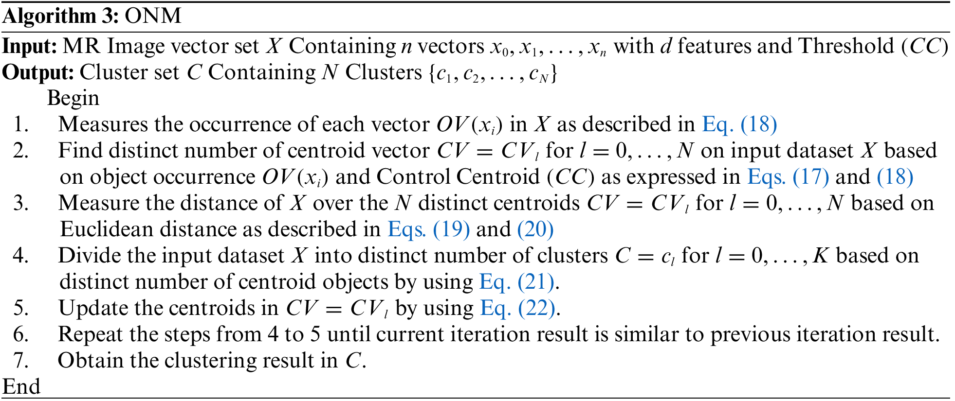
Similarly, in this subsection, the MIPC approach is partitioned the MRI image dataset into distinct number of different clusters based on improved partitioned clustering ONM scheme [25,26]. It consists of two stages likely dissimilar spatial centroid vector (DSCV) and partitioning respectively. In the DSCV stage, the ONM approach identifies the distinct number of centroid vectors over input MRI image vector set X=xi based on occurrence of objects in the dataset X. First, it computes rate of repetition of each spatial vector OV(Xi) over the dataset X=xi, for i=0,…,n and is defined in Eq. (17) as:

OV(Xi)=∑j=i+1n|xi−xj||∀xi,xj∈X,where{1|xi−xj|<T0|xi−xj|>T}(17)

where, xi and xj represent ith and jth vectors that belongs in to the MR image vector set X, n denotes the size of X and T is the threshold that limit the similarity distance between ith and jth vectors. If the difference of ith and jth objects is lesser than T, it means that the jth object is similar to ith object or vector that belongs to the MR image dataset X. In the second step, it finds the distinct number of different Centroid Vector (CV) in dataset X based on object occurrence OV(xi) and is computed by

CV={{OV(xi)i=1,…,n}∀OVi∈OV,where{xiOVi≥CC}}(18)

In this, OVi denotes the rate of occurrence of ith vector in X and CC represents the Control Centroid that intends to dynamically identify the appropriate number of spatial centroid vector in MRI image dataset X and is determined in form of CV=CVl, for l=1,…,N, f=1,2,…,d and l=1,…,N, where, CVl is in the partitioning stage, the ONM approach divides the MR image vector set into optimum number of N discrete clusters based on distinct centroid vectors. The clustering stage consists of three steps. In the first step, it measures the distance of each individual vector in vector set X over the N centroid vectors in CV=CVl for l=1,2,…,N and f=0,1,…,d based on Euclidean distance and is defined in Eq. (19) as

D(X,CV)={d(xi,CV)|∀xi∈X,∀CVl∈CV}(19)

where, d(xi,CVl) represents the Euclidean distance between ith vector in X and lth centroid in CV and is computed by

d(xi,COl)={(∑f=1D(xif−COlf)2)1/2}(20)

Here, xif denotes the fth feature of ith vector in X and CVlf represents the fth feature of lth centroid vector. Second step, it finds the closest centroid vector of each individual object in dataset X=xi with minimum Euclidean distance which computed at step 1 and respectively it assign the ith object in X into its closest lth cluster in cluster set C=cl for l=0,1,…,N and is defined in Eq. (21) as

Cl={min{D(xi,CVl)l=0,1,…,N}|∀xi∈X}(21)

In the last step, it modifies the centroid of each individual cluster in cluster set C=cl, for l=0,…,N and cl=clj for j=0,1,…,R and is defined in Eq. (22) as:

CVl={1Rl∑j=0Rlclj|∀cli∈cl,∀cl∈C}(22)

In this, cij denotes the jth object in lth cluster in cluster set C and Rl is the size of lth cluster in cluster set C.

6  Cluster Validation Stage

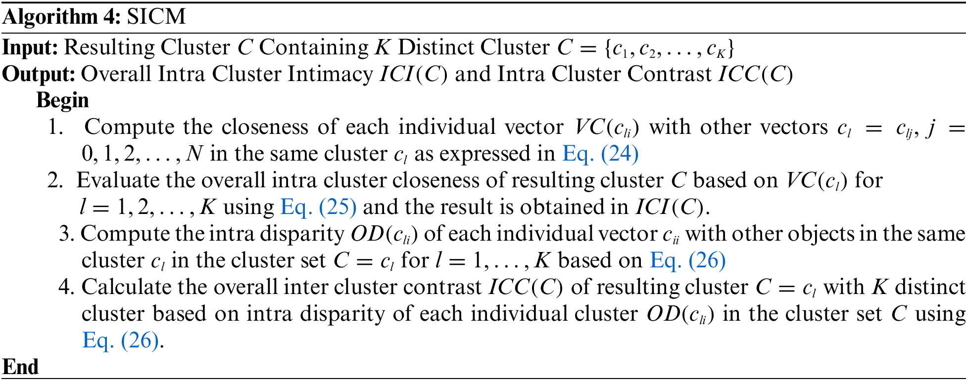
This stage presents, the MIPC scheme estimates the closeness and separation among the data objects in each individual cluster in the cluster set of MR image vector set based on proposed cluster validation scheme (SICM). The proposed (SICM) is an improved version of existing validation techniques as reported in [27–29] and it aims to validate the quality of each individual cluster in the cluster set of MR image that identified by MIPC scheme based on probability concept. The SICM consists of two measures Intra Intimacy (II) and Intra Contrast (IC). The II measure uses to estimate the closeness of each individual vector with other vectors in the same cluster OC(cli), where, cli represents the ith object in the lth cluster in cluster set C with K clusters and the vector closeness VC(cli) measure is defined in the Eq. (23) as

VC(ci)={{1|cl|∑i=1|cl|{{1|cl|∑j=1|Cl|∑f=14|clif−cljf|}×100}},∀clif∈cli,∀clj∈cl,∀cl∈Cwhere{1|clif−cljf|<=θ0|clif−cljf|>θ},{1∑f=14|clif−cljf|>=20∑f=14|clif−cljf|<2}}(23)

where, clif is the fth pixel value in jth vector in the lth cluster that belongs into the cluster set C for l=0,1,2,…,K, |cl| is the size of the lth cluster for j=0,1,2,…,N, θ denotes the predetermined threshold or constant that uses to limit the difference between two objects. Next, the IC calculates the overall intra cluster intimacy ICI among the cluster set C based on individual cluster closeness VC(cli) within the same cluster set and is defined in the Eq. (24) as

ICI(C)={1K∑l=0KVC(cl)}(24)

Similarly, the intra contrast measure aims to estimate the intra disparity among the vectors within the same cluster in the cluster set. First, it measures the intra disparity VD(cl) of each individual vector cl=clj for j=0,1,2,…,N with other vectors within the same cluster in the cluster set C=cl for l=0,1,2,…,K and it defined in the below given Eq. (25) as:

VD(ci)={{1|cl|∑i=1|cl|{{1|cl|∑j=1|Cl|∑f=14|clif−cljf|}×100}},∀clif∈cli,∀clj∈cl,∀cl∈Cwhere{1|clif−cljf|<=θ0|clif−cljf|>θ},{1∑f=14|clif−cljf|>=20∑f=14|clif−cljf|<2}}(25)

Subsequently, the IC measure estimates the overall intra cluster contrast ICC(C) over the cluster set C with K distinct clusters based on intra vector disparity VD(cl) of each individual cluster in the cluster set C=cl for l=0,1,2,…,K and is computed by,

ICC(C)={1K∑l=0KVD(cl)}(26)

7  Complexity Analysis

This section discovers the computational complexity of MIPC approach has tested over MR image dataset by three different improved unsupervised clustering schemes namely iLIAC, DAAC and ONM. The MIPC system consumes time O(nd) to split the digital MR image X into n non overlapping blocks or vectors with d pixels, where n is the number of vectors or blocks or vectors in the input digital MR image vector set X and is describes as X=xi for i=0,1,2,…,n, xi=xif for f=0,1,2,…,d. Ahmed et al. [30] have presented automatic segmentation and detection of brain tumor is a notoriously complicated issue in magnetic methods are limited for detection of tumor in multimodal brain MRI. This work analyses the segmentation performance of existing state of art method improved Fuzzy C-Means clustering (FCMC) method and marker-controlled watershed method to carry out accurate brain tumor detection and enhance the segmentation results. Next, the complexity analysis of MIPC system is performing in the clustering stage including different clustering schemes iLIAC, DAAC and ONM respectively as described in the below.

7.1 MIPC (iLIAC)

First, it requires time O(nd) to extract the single feature over each individual vector or block in the MR image vector set X=xi with n vectors based on Eq. (1) and the extracted features are obtained in dataset X¯=x¯i for i=0,1,2,…,n. Next, it consumes O(n) time to compute the control merge cost (ϕ) over the MR image feature dataset (X¯) with n data elements. Afterward, in the every iteration the iLIAC clustering scheme needs time O((n(n−1)/2)+1+1) to construct upper triangular distance matrix Ud(X¯) over the cluster set (X¯) with n clusters, identifies closest cluster pair (xi,xj) and update the cluster set (X¯) respectively. The MIPC system needs time O((n(n−1)/2)+1+1) for (n−K) iterations to identify the appropriate number of dissimilar clusters based on iLIAC scheme without user input. Overall the MIPC (iLIAC) system consumes time O((((n(n−1))/2)+1+1)(n−K)+(nd)) to process and identifies applicable number (K) of dissimilar clusters over the MR image vector set (X¯).

7.2 MIPC (DAAC)

In the first stage, the (DAAC) clustering scheme needs time O(nK) to identify number of distinct representative objects over the MR image feature set X¯=x¯i with n objects based on DROC method, where, K is the number of representative objects in image feature set (X¯). Next stage, it consumptions time O((n(n−1)/2)+1+1) to build upper triangular matrix over the MR image vector set X, identifies closest vector pair (xi,xj) with higher similarity and update the vector set X. Overall the MIPC (DAAC) scheme is required time O(((n(n−1)/2)+1+1)(n−K)+(nd)+(nK)) to identify finest number (K) of dissimilar clusters that belongs into the MR image vector set X without pre-determined knowledge, where, (n−K) is the number of iterations.

7.3 MIPC (ONM)

Initially, the (ONM) clustering scheme consumptions O(ndK) time to identify appropriate number of dissimilar centroid vectors over the MR image vector set X=xi, xi=xij, for i=0,1,2,…,n and j=0,1,…,d based on DCV method, where, K is the number of centroid vectors that belongs in to the vector set X. In the partitioning stage, the ONM scheme takes time O(ndKr) to iteratively split the MR image vector set X into finest number of K distinct highly relative clusters, where, r is the number of iterations. As a whole, the MIPC (DAAC) system has required time O(ndKr+ndK) to identify finest number (K) of dissimilar clusters that belongs into the MR image vector set X.

8  Results & Discussions

This section presents the MIPC approach, experimented on MR gray scale medical images based on three different improved unsupervised clustering schemes iLIAC, DAAC and ONM respectively. For the experimental purpose, we have taken 100 natural 100 2-D gray scale MR medical images with different sizes such as (120 * 120), (124 * 124) and (130 * 130) respectively and the grey values in the range 0–255.

A subset of this dataset containing ten sample standard MR brain and breast images via, Brain_1, Brain_2, Brain_3, Breast_1 and Breast_2 are reported as representative in this subsection. The sample MRI images are used in many research experiments as reported in (Lai & Huang 2011; Qi et al. 2015; Yong & Shuying 2007). Fig. 1 shows the five standard MRI gray scale images Brain_1, Brain_2, Brain_3, Breast_1 and Breast_2 as illustrated in Figs. 2a–2e respectively. In this experiment, each block of size (2 * 2) is considered as a vector and hence each sample image contains 3844, 4225, 3600, 3844 and 4225 vectors respectively.

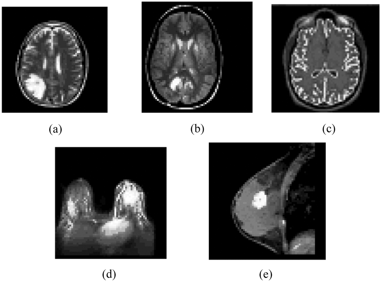
Figure 2: Result of the MIPC scheme tested on the ten gray scale images using iLIAC approach indicated in Fig. 1: (a) Result of brain_1 (b) Result of brain_2 (c) Result of brain_3 (d) Result of breast_1 (e) Result of breast_2

Firstly, the MIPC approach identifies distinct number of dissimilar clusters over the seven gray scale medical image datasets based on iLIAC scheme. Initially, it computes the control merge cost over seven gray scale MR images and the results are obtained in Tab. 1 as 7.87, 7.51, 7.71, 7.85, 7.44 respectively. Then it followed by computation of upper triangular distance matrix and in the case of sample gray scale MRI image datasets are presented in Fig. 2. The clustering scheme could identify 24, 25, 24, 25 and 25 distinct clusters over the MRI images in the Fig. 2. The results are incorporated in the Tab. 1. Fig. 3 demonstrates the clustering result of the iLIAC scheme has tested the MRI images likely Brain_1, Brain_2, Brain_3, Breast_1 and Breast_2 as obtained in Figs. 2a–2e respectively.

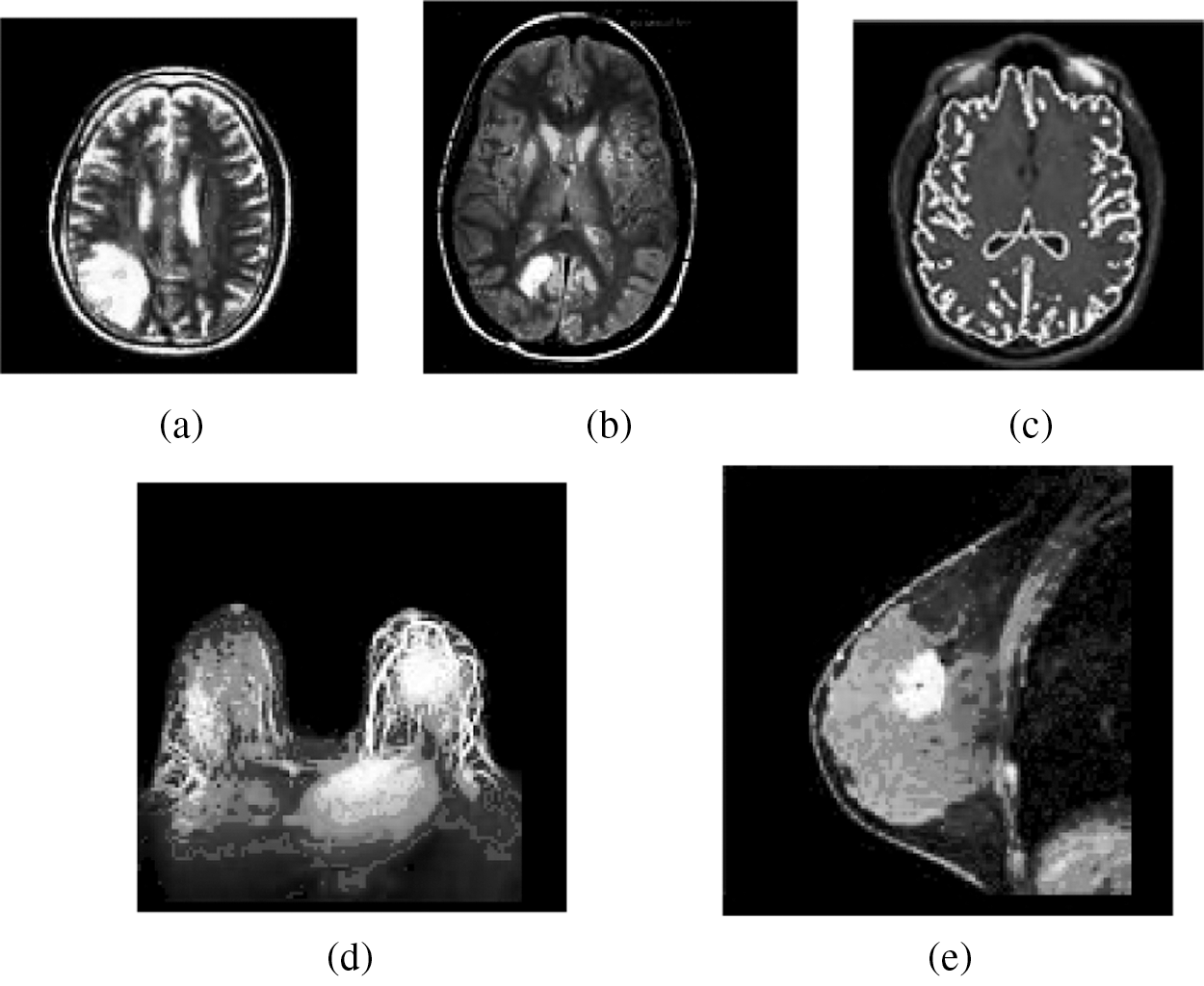
Figure 3: Result of the MIPC scheme tested on the ten gray scale MR images using DAAC approach indicated in Fig. 2: (a) Result of brain_1 (b) Result of brain_2 (c) Result of brain_3 (d) Result of breast_1 (e) Result of breast_2

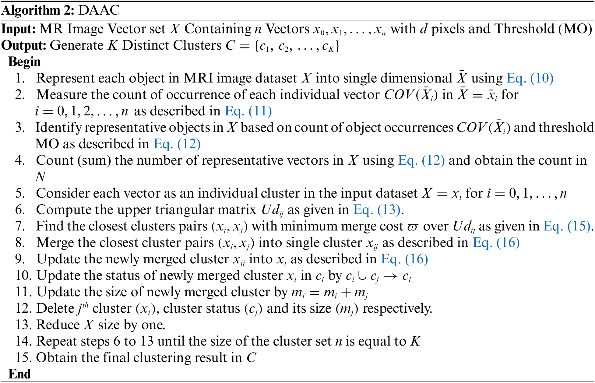
Similarly, the MIPC approach detects distinct number of unrelated clusters on same five MR image datasets based on DAAC scheme. Primarily, it automatically traces the distinct representative objects over the five MR images as illustrated in Fig. 2 based on frequency of maximum occurrence (MO = 15) and the count of distinct representative objects are obtained in Tab. 2 as 33, 27, 33, 39, 27 respectively. The Maximum Occurrence is a predetermined threshold which used to dynamically find the appropriate number of distinct representative objects in dataset. Then it followed by sequence of merging process and divides the each individual image dataset into distinct number of dissimilar clusters based on count of representative objects as presented in Tab. 3. In the case of sample gray scale image datasets presented in Fig. 3, the clustering scheme could identify 33, 27, 33, 39 and 27 distinct clusters. The resulting clusters of the clustering scheme are incorporated in the Tab. 2. Fig. 3 demonstrates the clustering result of the MIPC (DAAC) on five gray scale MR images Brain_1, Brain_2, Brain_3, Breast_1 and Breast_2 as obtained in Figs. 3a–3e, 3 respectively.

In the same way, the MIPC approach divides the MR image dataset into distinct number of discrete clusters based on ONM scheme. In the beginning, it robotically traces the distinct number spatial centroid objects on each individual gray scale MR image dataset based on control centroid (CC = 15) and the results are incorporated in Tab. 3. The Control Centroid (CC) is a user defined threshold that is used to generate the spatial centroid objects in dataset dynamically. Then it followed by iterative process and divides the each individual image dataset into distinct number of dissimilar clusters based on spatial centroid objects as presented in Tab. 3. The resulting clusters of the five gray scale MR images are incorporated in the Tab. 3. Fig. 4 demonstrates the clustering result of the MIPC (ONM) on five gray scale medical images Brain_1, Brain_2, Brain_3, Breast_1 and Breast_2 as obtained in Figs. 4a–4e respectively.

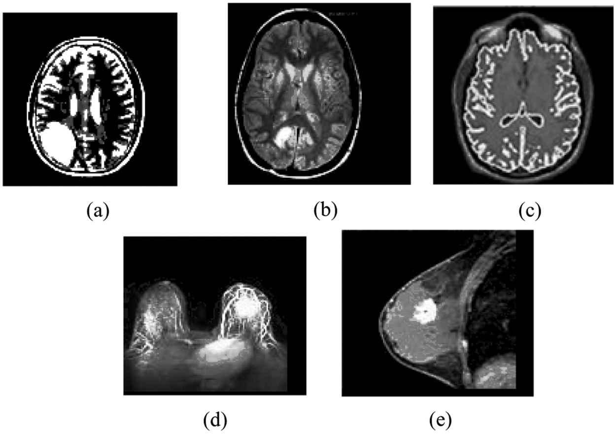
Figure 4: Result of the MIPC scheme tested on the ten MR images using DAAC approach indicated in Fig. 2: (a) Result of brain_1 (b) Result of brain_2 (c) Result of brain_3 (d) Result of breast_1 (e) Result of breast_2

The performance of the MIPC approach with three improved clustering schemes has been validated based on improved SICM schemes. It calculates the intra intimacy and intra cluster contrast over the each individual cluster in cluster set of MR images which tested by MIPC approach and the clustering results as shown in Tabs. 1–3 respectively. Initially, it measures the size of each individual cluster over the results of the five gray scale medical images Brain_1, Brain_2, Brain_3, Breast_1 and Breast_2 respectively. Next, it estimates the intra closeness (OC) and intra disparity (OD) in % among the individual cluster of these sample medical image datasets results based on the centroid of the each individual cluster.

Then, it followed to calculate the overall intra intimacy ICI(C) in % over the results of the MIPC approach with three different clustering schemes iLIAC, DAAC and ONM respectively. Subsequently, it produced 60.06, 56.43, 53.37, 73.39, 77.92; 77.28, 88.27, 77.27, 82.51, 85.39; 72.14, 73.58, 70.215, 79.17, 83.39 for the sample gray scale image datasets Brain_1, Brain_2, Brain_3, Breast_1 and Breast_2 respectively. The estimated results of sample medical image datasets as obtained in Tab. 4. Similarly, the overall intra cluster contras ICC(C) is calculated over the clustering results of MR images which obtained by MIPC scheme based on intra disparity measures.

The validation results of MR images which tested by iLIAC, DAAC and ONM clustering schemes are obtained in Tab. 5 as 39.93, 43.56, 46.62, 26.60, 22.075; 22.71, 11.72, 22.72, 17.48, 14.60 and 27.85, 26.41, 29.78, 20.82, 16.60 respectively. It is clearly shown in the performance measurement results as illustrated in Figs. 4, 5, and 6 that the proposed SICM has flawlessly estimated intra cluster intimacy and intra cluster contrast over the result of MR cancer image. Accordingly to the performance measurement results, that the DAAC clustering schemes has identified appropriate number of dissimilar groups (Normal & Abnormal regions) over the MR cancer images with good accuracy compared to ONM and iLIAC schemes without predetermined input. Similarly, the ONM scheme has produced better clustering results with higher intra closeness and lower intra contrast compared to iLIAC scheme.

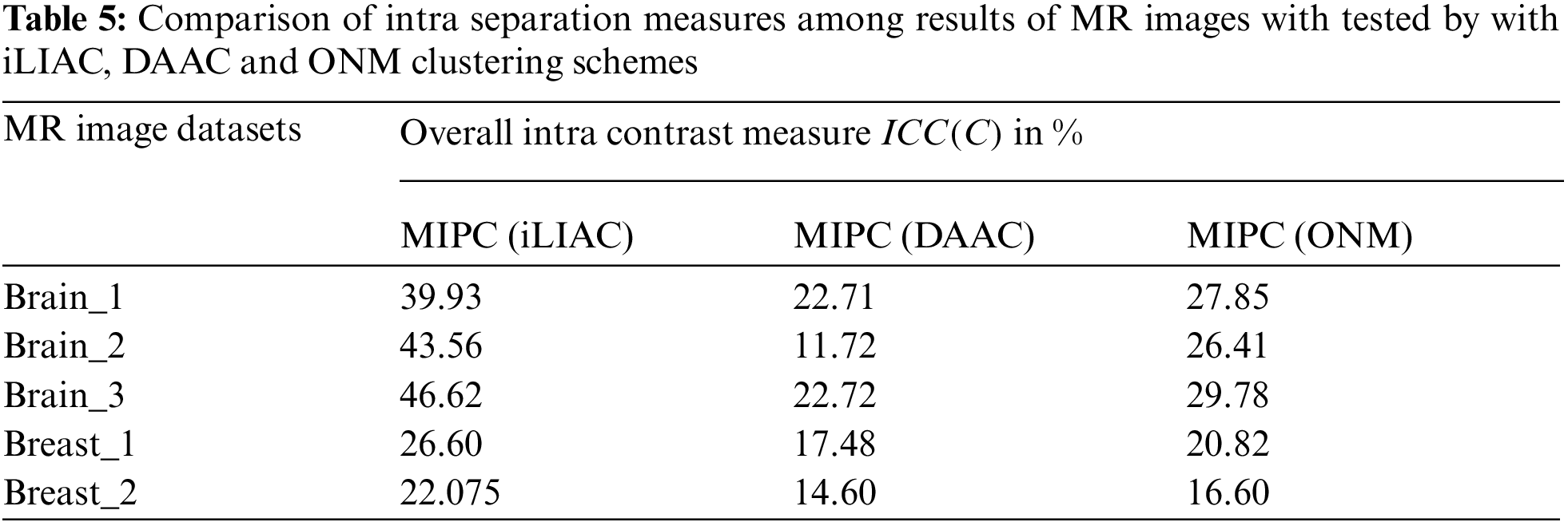
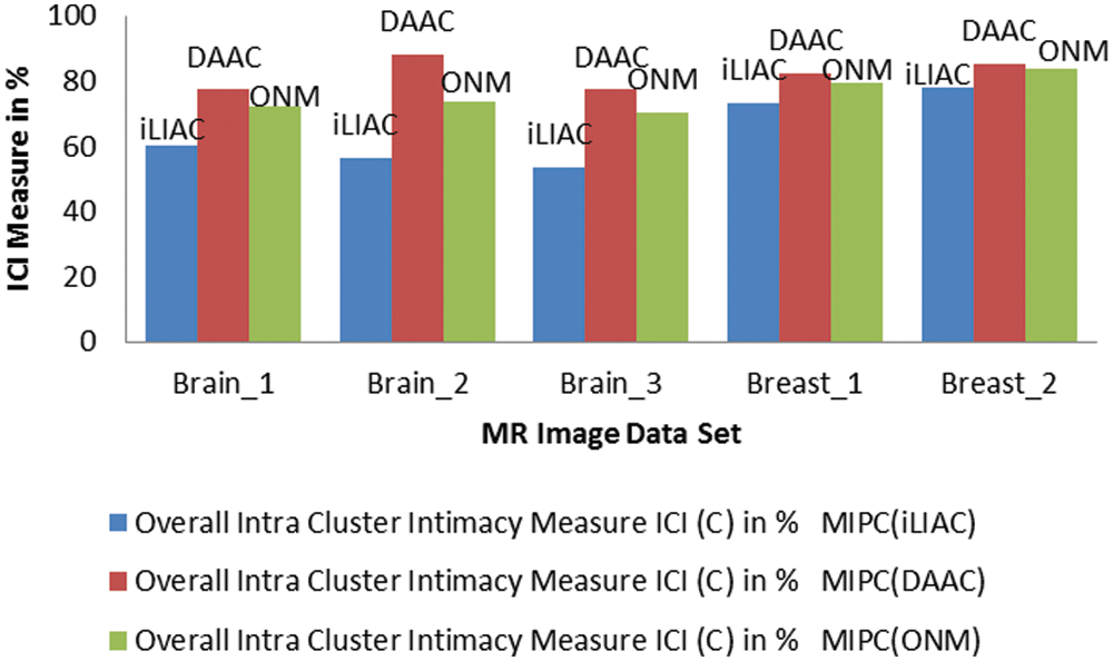
Figure 5: Comparisons of (ICI) performance measure over clustering results of MR images tested by improved unsupervised clustering schemes iLIAC, DAAC and ONM

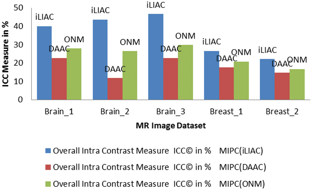
Figure 6: Evaluations of (ICC) performance measure over clustering results of MR images tested by improved unsupervised clustering schemes iLIAC, DAAC and ONM

9  Conclusion

This article presents Inherent Image Pixels Classification using three different improved unsupervised clustering schemes iLIAC, DAAC and ONM. The MIPC approach is aimed to trace the dissimilar pattern over the gray scale medical image through automatic identification of the distinct number of highly relative clusters in the medical image dataset based on improved unsupervised cluster schemes for deeper investigation and analysis. First, the MIPC approach automatically identifies the distinct number of dissimilar clusters over the medical image dataset based on three different clustering schemes iLIAC, DAAC and ONM in the separate manner. Next, the results of the MR images are validated based on proposed SICM scheme. We tested the MIPC approach with three improved unsupervised clustering schemes on five gray scale cancer MR images likely Brain_1, Brain_2, Brain_3, Breast_1 and Breast_2. According to the experimental results, the MIPC approach is more efficient and effective for automatic identification of the maximum number of highly relative clusters including normal and abnormal regions over the gray-scale MR cancer image with higher intra intimacy and lower intra contrast. After conducting various experiments, we concluded that the MIPC approach is better suitable to identify appropriate number of dissimilar regions (normal & abnormal), improving clusters quality and validate the clustering result for plateful to investigate (normal & abnormal regions) the dissimilar patterns in the MR cancer images.

Acknowledgement: This work is supported by Faculty of Science and Technology, University of the Faroe Islands, Faroe Islands, Denmark and REVA University, Bengaluru. The authors like to extend thanks to reviewers and experimental continuation of experts in this research.

Funding Statement: The authors received no specific funding for this study.

Conflicts of Interest: The authors declare that they have no conflicts of interest to report regarding the present study.

This work is licensed under a Creative Commons Attribution 4.0 International License, which permits unrestricted use, distribution, and reproduction in any medium, provided the original work is properly cited.