LCF: A Deep Learning-Based Lightweight CSI Feedback Scheme for MIMO Networks

Kyu-haeng Lee

doi:10.32604/cmc.2022.024562

Dankook University, Yongin-si, Gyeonggi-do, 16890, Korea
*Corresponding Author: Kyu-haeng Lee. Email: kyuhaeng.lee@dankook.ac.kr
Received: 22 October 2021; Accepted: 26 November 2021

Abstract: Recently, as deep learning technologies have received much attention for their great potential in extracting the principal components of data, there have been many efforts to apply them to the Channel State Information (CSI) feedback overhead problem, which can significantly limit Multi-Input Multi-Output (MIMO) beamforming gains. Unfortunately, since most compression models can quickly become outdated due to channel variation, timely model updates are essential for reflecting the current channel conditions, resulting in frequent additional transmissions for model sharing between transceivers. In particular, the heavy network models employed by most previous studies to achieve high compression gains exacerbate the impact of the overhead, eventually cancelling out the benefits of deep learning-based CSI compression. To address these issues, in this paper, we propose Lightweight CSI Feedback (LCF), a new lightweight CSI feedback scheme. LCF fully utilizes autoregressive Long Short-Term Memory (LSTM) to generate CSI predictions and uses them to train the autoencoder, so that the compression model could work effectively even in highly dynamic wireless channels. In addition, 3D convolutional layers are directly adopted in the autoencoder to capture diverse types of channel correlations in three dimensions. Extensive experiments show that LCF achieves a lower CSI compression error in terms of the Mean Squared Error (MSE), using only about 10% of the overhead of existing approaches.

Wireless communication systems have significantly benefited from utilizing Channel State Information (CSI) at the transmitter. As one indicator of CSI, the Signal-to-Interference-plus-Noise Ratio (SINR) has been used to enable intelligent transmission functionalities such as dynamic data rate adaptation, admission control, and load balancing since the early days of wireless communication. With the advent of the Multi-Input Multi-Output (MIMO) method, which has now become a core underlying technology in most current systems, such as 5G and Wi-Fi [1,2], the importance of CSI at the transmitter has been highlighted, since proper MIMO beamforming weights can be calculated only through CSI values that accurately reflect the attenuation of the actual channel between a transmitter and a receiver. For this reason, both cellular and Wi-Fi systems already operate their own CSI feedback protocols to allow the transmitter to acquire channel information a priori.

A CSI feedback process is essential for modern communication systems, yet it faces a critical overhead issue that could greatly limit the potential of MIMO beamforming gains. The amount of CSI that needs to be sent to the transmitter is basically proportional to the number of transmitting and receiving antennas; in Orthogonal Frequency Division Multiplexing (OFDM) systems, the number of subchannels also contributes to an increase in the feedback size, since CSI for every subchannel is required for OFDM transmission. Moreover, for reliable CSI feedback, CSI is typically transmitted at low data rates (e.g., 6.5 Mbps over Wi-Fi), which further exacerbates the impact of the overhead. According to a study, the overhead can reach up to 25 × the data transmission for a 4 × 4 160 MHz Wi-Fi MIMO channel [3], and such substantial overhead will not only limit the network capacity but also prevent the realization of advanced MIMO functionalities, such as massive MIMO, distributed MIMO, and optimal user selection [4–7].

Thus far, numerous schemes have been proposed to address the CSI feedback overhead problem. One widely accepted idea is to exploit the diverse types of channel correlation that could be readily observed in the temporal, frequency, and spatial domains. The channel coherence time has been used to eliminate unnecessary CSI feedback transmissions in many studies [3,8–10], and similarly adaptive subcarrier grouping is employed to reduce the feedback size in OFDM systems [3,10]. A rich body of literature focuses on utilizing the spatial channel correlation used in multi-antenna communication for the same purpose [10–12]. Recently, as deep learning technologies have received attention for their superior ability to extract the principal components of data, there have been many efforts to apply them to CSI compression [13–18] and estimation [19–23]. In particular, in this field, autoencoders are commonly employed: A receiver compresses CSI data with the encoder of an autoencoder, and the transmitter reconstructs the original CSI using the decoder. A novel CSI compression scheme, CSINet [13], is built on a convolutional autoencoder, where the authors regard the CSI compression problem as a typical 2D image compression task. Along this line, numerous variants of CSINet have been developed for various purposes [14–17].

Although the aforementioned approaches show that deep learning can be used as a very effective tool for CSI compression, there still remain several critical issues to be solved in terms of how the transceivers can practically share the models. Neural network-based CSI compression schemes are basically premised on sharing a model between a transmitter and a receiver, which means that some transmissions for this model sharing, and their accompanying cost, are unavoidable. In this paper, we refer to this as model sharing overhead. Unfortunately, this overhead has not been thoroughly taken into account in most existing studies, and in many cases, it is assumed that the transceivers already share a model or that model sharing will rarely happen. However, as we will see later, model sharing can occur quite often in practice, since the model cannot guarantee a high degree of generalization to wireless channel data. If the model cannot properly cope with CSI values that it has not experienced during training, then the compression and recovery will fail, which leads to an inevitable process of model re-training and sharing. Of course, in some channel environments where a clear pattern is found, as shown in Fig. 1a, the overhead problem may not be so serious. However, this situation cannot be always guaranteed; the actual channels may look more like the one in Fig. 1b. In addition, due to the strong randomness of the change in the wireless channel state, simply increasing the amount of training data does not result in noticeable generalization enhancement. Rather, it is more important to use a proper set of training data that reflects the pattern and tendency of the current channel status well, and for this, an appropriate channel status prediction can be of great help.

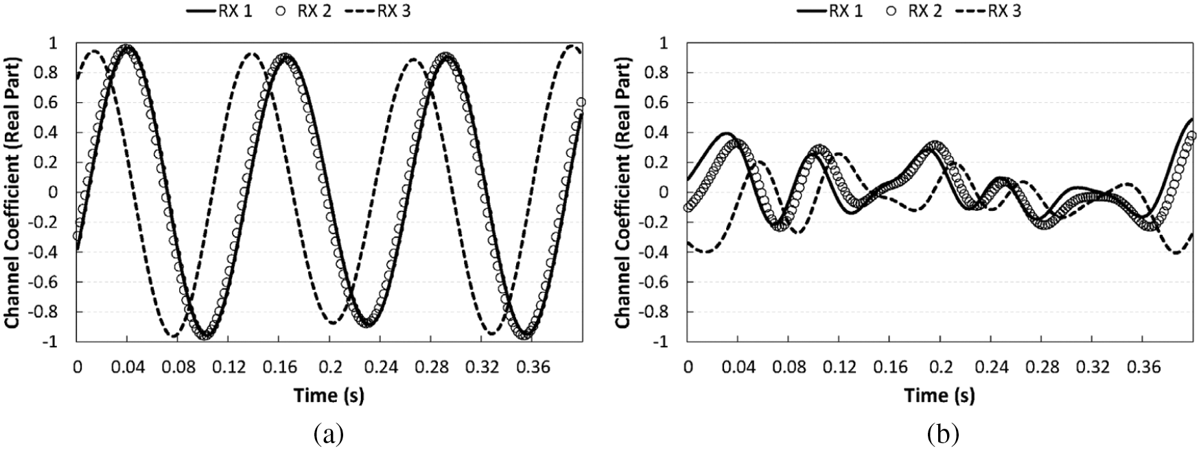
Figure 1: Examples of channel coefficient changes over time for two scenarios. Only the real parts of the complex channel coefficients of the first path between the first transmitting antenna and three receiving antennas are displayed. (a) Stable channel case (b) Dynamic channel case

As mentioned earlier, most of the previous approaches focus only on making the model work at higher compression ratios, and thus they prefer deep and wide networks in their designs. For example, CSINet [13] uses five convolutional layers and two fully connected layers, and it successfully compresses CSI with a high compression ratio of up to 1/64, which obviously outperforms conventional compressed sensing-based approaches [24,25]. However, from the model sharing perspective, the model is still too big to share; roughly calculated, for an 8 × 2 MIMO channel with 8 paths, it needs more than 1,000 decoder parameters in total, which actually makes it larger than the original CSI (i.e., 256 = 8 × 8 × 2 × 2, where the last number denotes the real and imaginary parts of complex channel coefficients). In this case, model sharing is practically not available since it consequently cancels out the benefits of compression.

In order to overcome these limitations, in this paper, we propose a lightweight CSI feedback scheme (LCF). Similar to recent approaches, LCF exploits deep neural networks to achieve better CSI compression, but we focus more on ensuring that the model does not impose a substantial burden on the network when being shared. LCF mainly consists of two parts: CSI prediction and CSI compression. First, for CSI prediction, LCF employs a long short-term memory (LSTM) structure to infer future CSI values, which are in turn used to train the CSI compression model. In particular, to generate multiple future CSI predictions effectively, we apply an autoregressive approach to our model. The actual channel compression and reconstruction is conducted by a convolutional autoencoder, where 3D convolution layers are adopted to capture channel correlations in the three dimensions of the transmitting antenna, receiving antenna, and path delays. The resulting compression model appears to be simple compared to recent proposals; however, we will show that this lightweight network structure is still sufficient for achieving high CSI compression performance, with a much cheaper model sharing overhead.

The proposed CSI feedback scheme is developed and evaluated in a TensorFlow [26] deep learning framework. In order to investigate the performance of LCF for various channel environments, we simulate channel coefficients by applying the WINNER II channel model [27,28]. We provide micro-benchmarks that evaluate the performance of each CSI prediction and compression process, and we compare the overall performance of LCF with those of AFC [3] and CSINet [13] in terms of CSI recovery accuracy and model sharing overhead. Through extensive experiments, we show that LCF obtains more stable and better CSI compression performance in terms of the mean squared error (MSE), with as low as 10% of the model sharing overhead of the existing approaches. We summarize the main contributions of this paper as follows:

1. We propose a novel deep learning-based CSI feedback scheme, LCF, which effectively reduces the CSI feedback overhead by using CSI prediction based on autoregressive LSTM and CSI compression with a convolutional autoencoder. We propose the use of CSI predictions to train the autoencoder, so that the compression model can be valid even in highly dynamic wireless channels.

2. We design a CSI feedback algorithm to make the transmitter and the receiver effectively share the compression model, which has not been investigated well in previous studies. The proposed algorithm can be applied to the existing deep learning-based CSI compression approaches as well.

3. The performance of LCF is evaluated for various wireless channel scenarios using the WINNER II model, and it is also compared with those of other approaches through extensive experiments. LCF shows more stable and better CSI compression performance, using only about 10% of the overhead of existing approaches.

The rest of this paper is organized as follows. In Section 2, we review the previous works related to this paper. In Section 3, we provide the preliminaries of this work, and Section 4 describes LCF in detail. Section 5 evaluates the performance of the proposed scheme, and we conclude this paper in Section 6.

Numerous schemes have been proposed to address the CSI feedback overhead problem using diverse types of channel correlations. The channel coherence time, during which the channel state remains highly correlated, has been used as a key metric for eliminating unnecessary CSI feedback transmissions in many studies [3,8–10,12]. Huang et al. [8] analyze the effect of time-domain compression, based on a theoretical model of channel correlation over time. Sun et al. [9] simulate the 802.11n single-user MIMO (SU-MIMO) performance in time-varying and frequency-selective channel conditions. AFC [3] computes the expected SINR by comparing the previous and the current CSI values and then utilizes it to determine whether to skip a CSI feedback transmission or not.

Similar ideas can be applied to compressing the frequency domain CSI values. Since in OFDM systems, the channel estimation should be performed on each subcarrier, appropriate subcarrier grouping can reduce the feedback size significantly. In MIMO systems, spatial correlation could also be used for CSI compression. Gao et al. [10] design a channel estimation scheme for an MIMO-OFDM channel using both temporal and spatial correlations. Ozdemir et al. [11] analyze the parameters affecting spatial correlation and its effect on MIMO systems, and Karabulut et al. [12] investigate the spatial and temporal channel characteristics of 5G channel models, considering various user mobility scenarios. These schemes can be further improved with proper quantization schemes that encode the original CSI data with a smaller number of bits. AFC [3] employs an adaptive quantization scheme on top of the integrated time and frequency domain compression, and CQNET [14] is designed for optimizing codeword quantization using deep learning for massive MIMO wireless transceivers. Among other things, it is actually being used for codebook-based CSI reporting in current cellular and Wi-Fi systems [1,2].

Recently, as deep learning technologies have received attention for their powerful performance in extracting the principal components of data, there have been many efforts to use this capability for CSI compression [13–18] and estimation [19–23]. The autoencoder model is widely used in this field since it best fits the problem context. A novel CSI compression scheme, CSINet [13], uses a convolutional autoencoder to solve the CSI compression problem by turning it into a typical 2D image compression problem. Along this line, numerous variants of CSINet have been developed so far [14–18]. RecCsiNet [15] and CSINET-LSTM [16] incorporate LSTM structures into the existing autoencoder model to benefit from the temporal and frequency correlations of wireless channels. The authors of PRVNet [17] employ a variational autoencoder to create generative models for wireless channels. In DUalNet [18], the channel reciprocity is utilized for CSI feedback in FDD scenarios. Most of these approaches validate the feasibility of deep learning as an effective tool for CSI compression and feedback; however, there remain several practical open issues related to model sharing and generalization, which will be discussed in the following section.

In this section, we describe the channel model and propagation scenarios used in this paper, and we explain the model sharing overhead problem, which motivates this work, in greater detail.

We consider an SU-MIMO communication scenario in which a receiver equipped with Nr antennas feeds the estimated CSI back to its transmitter, which is equipped with Nt antennas. Uniform Linear Array (ULA) antennas with 2 cm spacing are assumed for both the transmitter and the receiver. For simplicity, moving network scenarios are not considered. In order to simulate channel coefficients for diverse channel environments, we adopt the WINNER II channel model [27–31], which has been widely used in wireless communication research activities; it was recommended as a baseline for measuring radio communication performance in ITU-R (International Telecommunication Union-Radio communication sector) [29,30]. According to this model, the channel coefficients are generated based on a Clustered Delay Line (CDL) model (Fig. 2), where the propagation channel is described as being composed of a number of separate clusters with different rays, and each cluster has a number of multipath components that have the same delay values but differ in the Angle-of-Departure (AoD) and Angle-of-Arrival (AoA).

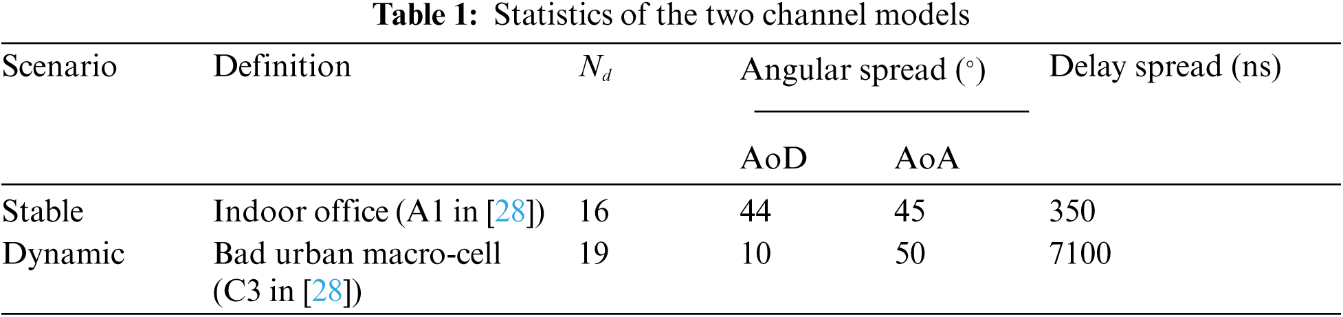
In this paper, we consider two different propagation scenarios, namely “stable” and “dynamic” scenarios, which model indoor office environments and bad city macro cells, respectively. Here, the former, as the name suggests, has a smaller channel status variation than the latter. Tab. 1 shows the basic statistics of the two channels. We use MATLAB to gather channel coefficient data for each case, and CSI data is sampled every 2 ms at the center frequency of 5.25 GHz. Note that MATLAB provides a toolbox for working with the WINNER model [27], which allows us to freely customize network configuration such as sampling rate, center frequency, number of base stations and mobile stations, and their geometry and location information. In particular, since the main channel parameters for various radio propagation scenarios defined by the WINNER model are already configured, the corresponding channel coefficient values can be easily obtained through this. 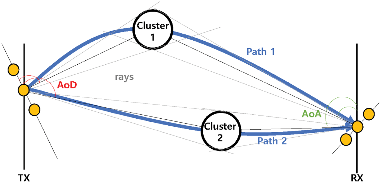For each scenario, channel coefficient data is expressed as a four-dimensional normalized complex matrix whose shape is (Ns×Nd×Nt×Nr), where Ns is the length of the sampled data and Nd is the number of path delays. Throughout this paper, we use the terms “CSI” and “channel coefficients” interchangeably.

Figure 2: Concept of the Clustered Delay Line (CDL) model [28]. Each cluster has a number of multipath components that have the same delay values but differ in the angle-of-departure and angle-of-arrival

To show the difference between the two scenarios, we plot the changes over time of the channel coefficients for each scenario in Fig. 1. These channel coefficients are the values corresponding to the first path of receiving antennas 1–3 and transmitting antenna 1, and only the real parts of these values are displayed in the plot. From the figure, we can observe the spatial and temporal correlation of the channels for both scenarios, even though they differ in degree. In the case of the stable channel scenario (Fig. 1a), similar signal patterns are repeated quite clearly over time and also among the three receiving antennas. In the case of the dynamic channel scenario (Fig. 1b), it is difficult to find a clear pattern like that in the previous case, yet we can still see correlations in the two domains.

We can see the difference between the two channels in terms of correlation more clearly in Fig. 3. In this figure, we measure the correlation coefficient of any two CSI instances separated by T, using the following formula [3,32]:

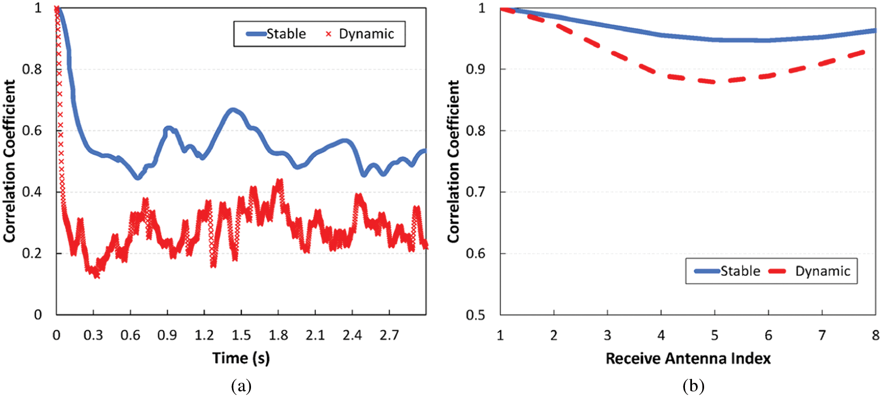
where L is the total length of CSI instances and h(t) is the CSI instance at time t. Note that the above equation can be also applied to computing the correlation in the spatial domain (Fig. 3b) by changing the definition of the separation. As expected, the stable scenario has overall higher temporal correlations than the dynamic channel, as shown in Fig. 3a; their coherence times1 are 420 and 40 ms, respectively. Compared to the temporal correlation result, higher spatial channel correlations among receiving antennas are observed in both cases (Fig. 3b), though the degree of correlation in the stable channel is still higher than that in the dynamic channel.

Figure 3: Temporal and spatial correlation of the two channels used in this paper. (a) Temporal correlation (b) Spatial correlation

As we saw earlier, wireless channels are basically diverse, and their characteristics are thus hard to generalize; some channels remain highly correlated over time for long periods of time, e.g., the stable channel, while others may experience large channel fluctuations, e.g., the dynamic channel. This aspect, unfortunately, has not been fully taken into account in most of the previous deep learning-based CSI compression schemes, although this leads to a substantial model sharing overhead that eventually limits the gains of deep learning. To identify the model sharing overhead in more detail, we revisit the CSI compression performance of CSINet [13] for three different channel environments, including the two channels described in the previous subsection. As a baseline, we additionally consider a purely random channel, where the channel coefficients are sampled from the normal distribution with zero mean and a variance of 0.1. Note that the stable channel used in this paper belongs to an ideal case in which we can readily predict how the channel changes in the future, while the random channel can be viewed as being at the other end of the spectrum. The mean squared error (MSE) in Section 5 is used as a performance metric, and we train the model using Adam optimization [34] with 10,000 CSI datasets and a maximum of 1,000 epochs.

First, Fig. 4a shows the compression performance according to varying compression ratios. What we pay attention to here is the performance in the dynamic channel: It deteriorates rapidly with the compression ratio, and its MSE value reaches 0.1 even at the low compression ratio of 1/8, which is too large to be used practically. Throughout this paper, the compression failure criterion, denoted as δthr, is set to the MSE of 0.1, and considering that for any wireless channels, the performance of CSINet will be somewhere between the two curves of the stable (i.e., blue curve) and the random (i.e., black dotted curve) channels, we can conclude that it is practically available only with the compression ratio of 1/8. When compression fails, the model has to be retrained and shared between the transceivers again, which eventually causes additional transmissions, i.e., model sharing overhead. Unfortunately, most of the previous approaches focus only on making the model work at higher compression ratios, and thus they prefer deep and wide networks in their designs, hoping that model sharing will not occur frequently. However, as can be seen, it could occur very frequently. In the case of the dynamic channel, at compression ratios greater than 1/16, for every CSI sample the model will always produce a high recovery error above the threshold; in this case, its heavy network structure will accelerate the feedback overhead increase.

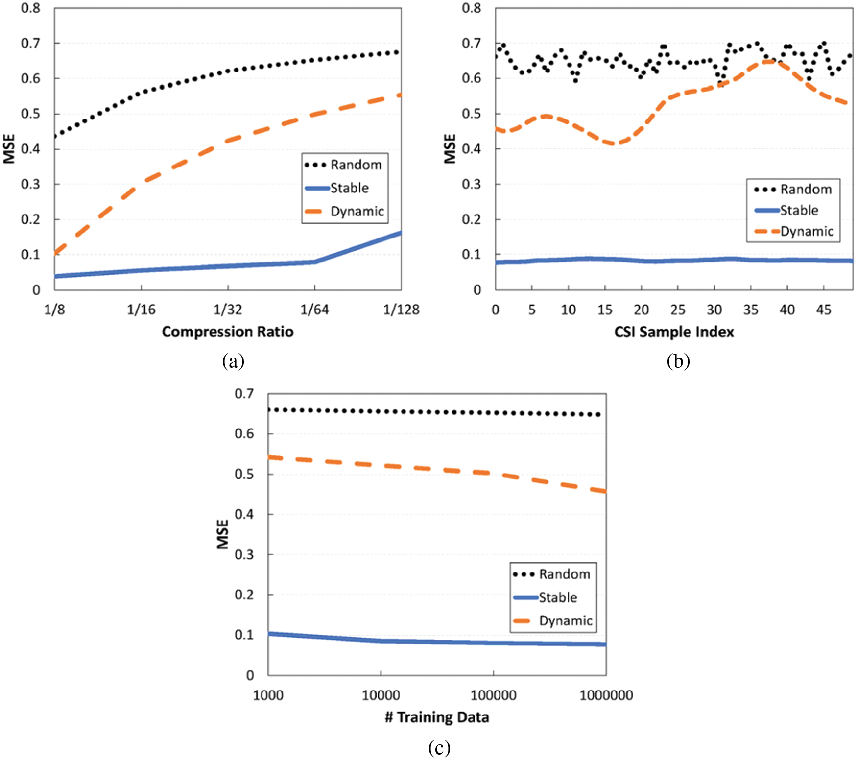
Figure 4: Performance of an existing deep learning-based CSI compression scheme for various channel environments. (a) MSE vs. Compression ratio (b) MSE vs. Time (c) MSE vs. Amount of training data

Therefore, we have to consider proper model sharing when designing a deep learning-based CSI compression scheme. Fig. 4 shows the result when 50 consecutive CSI values are compressed with a fixed model. If the channel is quite reliable, such as in the stable channel case, we might keep the high compression gains of deep learning, but this is not always guaranteed; as can be seen in the dynamic channel case, high recovery errors could continue over time, thus leading to additional feedback transmissions. One might think that this problem can be solved through training the model with more data and thus strengthening the model generalization. Unfortunately, this approach may not be very effective when dealing with wireless channel data, which generally have large irregularities over time. As shown in Fig. 4, even if we increase the number of CSI training data samples, there are only slight performance gains. In this case, the amount of training data may not be that important; rather, it is more important to use a proper set of training data that reflects the pattern and tendency of the current channel status well, and for this, appropriate channel status predictions could be very helpful.

We describe the proposed CSI feedback scheme in detail in the following section.

In this section, we provide an overview of the proposed scheme. As mentioned before, LCF is composed of two main processes, as shown in Fig. 5, for which different deep learning models are used: 1) autoregressive LSTM is used for CSI prediction, and 2) a convolutional autoencoder is used for CSI compression and reconstruction. In the first process, as the name suggests, a receiver generates predictions for future channel states using accumulated CSI values, which in turn will be used as the training dataset for autoencoder optimization. This process is described in detail in Section 4.2. Next, in the second step, the actual CSI compression and recovery is performed. Using the encoder of the autoencoder, a receiver compresses the estimated CSI into an M-byte codeword and then sends it back to the transmitter. Upon receiving the compressed CSI, the transmitter reconstructs the original CSI with the decoder of the autoencoder, which has been already shared by the receiver. More details on the compression model will be described in Section 4.3. Ideally, the feedback process of LCF requires only an M-byte data transmission, and therefore the feedback overhead can be significantly reduced. However, as mentioned earlier, such a gain is not always achievable; in some channel environments, the compression model could quickly become less effective and invalid. To tackle this issue, in LCF, a receiver dynamically updates and shares the compression model depending on the expected CSI recovery error obtained during the CSI compression. We explain this in more detail in Section 4.4.

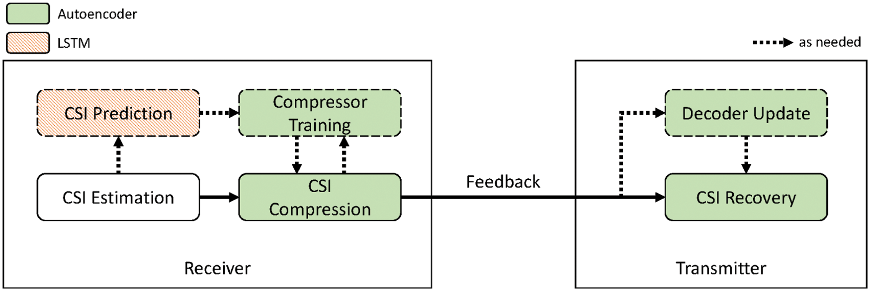
Figure 5: Overall structure of LCF. It consists of an LSTM-based CSI prediction process and an autoencoder-based CSI compression and reconstruction process. Note that the modules in the dotted box are executed as needed

Let Hi be the complex channel coefficient matrix whose shape is (Nd×Nt×Nr) at time slot i, and assume that a receiver keeps accumulated CSI matrices, denoted as H→a. Note that the superscript → is used to denote a vector. The objective of this step is to generate CSI predictions for the next No≥1 time slots, denoted as H→a=[H~i+1,H~i+2,…,H~i+No]T. To do this, we employ an autoregressive LSTM model as shown in Fig. 6. Let fLSTM and θLSTM be the model and its parameters, respectively. Then, we have H→o=fLSTM(H→i;θLSTM), where H→i, which is part of H→a, is the vector of the last Ni CSI samples. Note that H→a is updated whenever a new CSI sample is obtained. In this approach, the output of the model is repeatedly fed back into the model as input to generate its next prediction. For example, the prediction for time slot i+1, i.e., H~i+1, is in turn used to predict the next CSI value, H~i+2. This process is repeated until all No target CSI predictions are made.

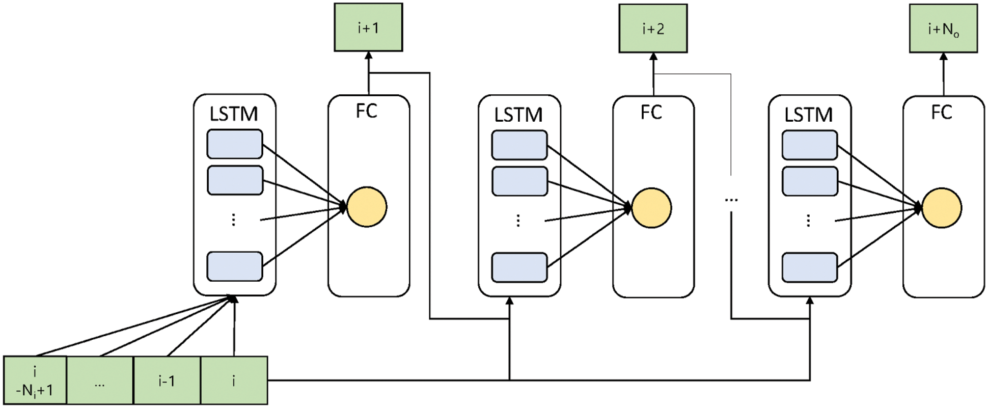
Figure 6: Autoregressive LSTM for CSI prediction. CSI predictions are made for each combination of the path delay, transmitting antenna, and receiving antenna

The proposed prediction model has two layers, an LSTM layer and a fully connected layer, as shown in Fig. 6. CSI predictions are made for each combination of the path delay, transmitting antenna, and receiving antenna. Additionally, we handle the real and imaginary parts of complex channel coefficients separately, since complex numbers are inherently not comparable in size and thus cannot be directly used in optimization. That is, we use 2NdNtNr models in total, and each model is used to generate CSI predictions for the corresponding combination. The input data shape for the models is (batch ×Ni×1), where the last number indicates the number of units (features) in the fully connected layer. One distinct feature of CSI data is that input data samples keep arriving sequentially to the model, and relatively old data samples can quickly become less effective. In this case, we can use online learning; instead of always training on the entire data set, i.e., H→a, in most cases, training is performed only on a small data set containing new data samples, i.e., H→i. In particular, the weights obtained in the previous step can be reused for performance. We basically use the MSE as the objective for optimization and employ Adam optimization [34].

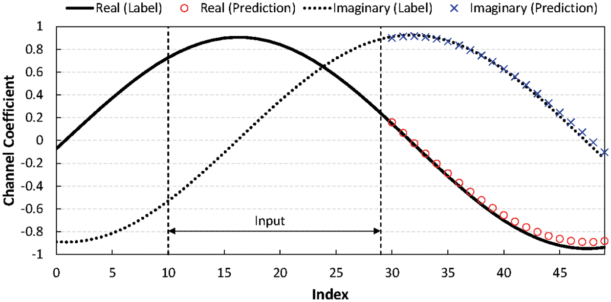
For better understanding, we illustrate an example of CSI prediction in Fig. 7. The channel coefficients shown in the figure are sampled from the channel of the first path between transmitting antenna 1 and receiving antenna 1 in the stable channel case. We depict two curves for both the real and imaginary parts of the channel coefficients in the figure. This example corresponds to the case of Ni=No=20, which means the channel coefficients from index 10 to index 29 are used to generate the next 20 CSI values from index 30 to index 49. As expected, the prediction performance is basically dependent on the previous prediction results; errors are continuously accumulated as predictions are made, and thus the prediction accuracy gradually drops as time advances. Starting from the MSE of 0.0001, the gap between the actual data and the prediction becomes apparent continuously, and at the last position, it grows to up to 0.0032. However, we note that this level of error is acceptable for the training data, as we will see later.

Figure 7: CSI prediction example for the channel of the first path between transmitting antenna 1 and receiving antenna 1

The proposed CSI compression model has the typical structure of an autoencoder, as shown in Fig. 8. It consists of two parts: An encoder and a decoder. Let fenc and fdec be the encoder and the decoder, respectively. The encoder takes the current CSI (i.e., Hi) as input, which is a four-dimensional channel coefficient matrix whose shape is (Nd×Nt×Nr×2), where the last element denotes the real and the imaginary parts. The first layer in the encoder is a 3D convolution layer, where three-dimensional filters are used to capture the channel correlation in both the spatial (for both the transmitting and receiving antennas) and delay domains. By default, we use 16 (3×3×3) filters, and the LeakyReLU activation function with a parameter of 0.3 is applied. Stripping is not used. The feature maps acquired from this layer are then transferred to a fully connected layer with M units through average downsampling with a shape of (2×2×2) and flattening, and thus the M-byte compressed CSI, denoted as HM, can be obtained as a result, i.e., HM=fenc(Hi;θenc), where θenc is a set of the encoder parameters.

The decoder is basically the mirror of the encoder. It first passes the encoded data (i.e., HM) to a fully connected layer with Nf units, where Nf is the size of the output of the convolution layer in the encoder, and then transfers the outcome to a convolution layer through the upsampling layer. Like the convolution layer in the encoder, the convolution layer in the decoder also takes three-dimensional filters; however, we employ a transposed convolution layer in the decoder to match the input shape and the output shape, i.e., (Nc×Nt×Nr×2). The same LeakyReLU activation function is applied, and L2 regularizers with a parameter of 0.001 are applied to all layers in the model. As a result, the decoder reconstructs the original CSI data from the compressed data, HM; that is, H^=fdec(fenc(Hi;θenc);θdec)=fdec(HM;θdec), where θdec is the decoder parameters. In the following subsection, we will explain how the model parameters (θenc and θdec) are trained and shared between transceivers.

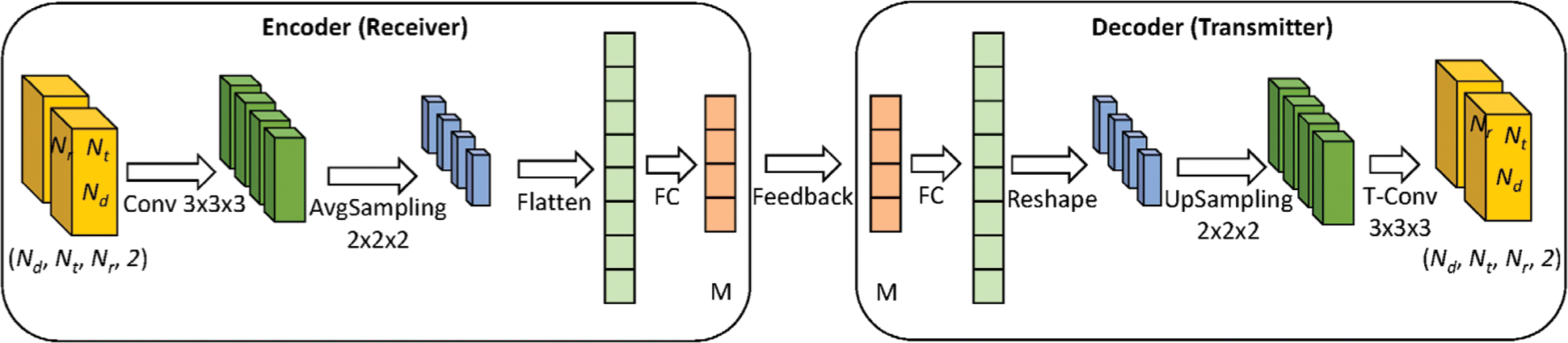
Figure 8: The proposed CSI compression and reconstruction model. 3D convolution layers are adopted in both the encoder and decoder

In LCF, the whole parameters of the autoencoder (both θenc and θdec) are trained by a receiver, but only the decoder parameters (θdec) are sent to the transmitter if needed. At the very beginning, the receiver trains the autoencoder with (No+1) CSI values, including the current CSI, i.e., Hi, and the newly generated No CSI predictions, i.e., H→o, and through this step, it obtains the trained encoder and decoder parameters, respectively. Since the decoder model is updated, its parameters need to be sent to the transmitter by the receiver. Now, the process of compressing the target CSI is conducted by re-training the model on it. Note that in this step, training is performed with the decoder parameters fixed, since the decoder parameters are already shared with the transmitter. In this process, θenc parameters are still trainable, so they may have different values before and after training. However, since they are not shared with the transmitter and are used only by the receiver, they do not have a significant impact on the system as a whole.

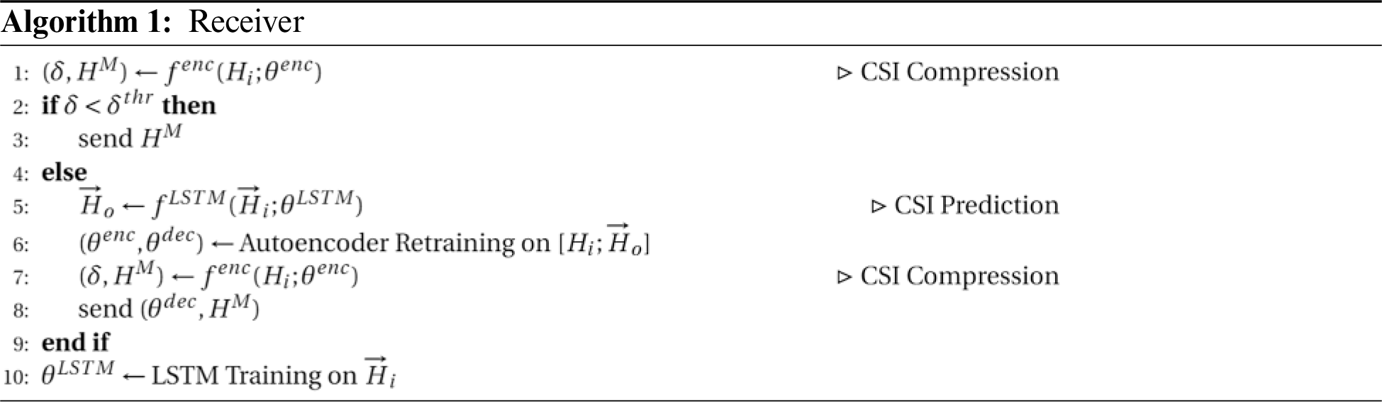
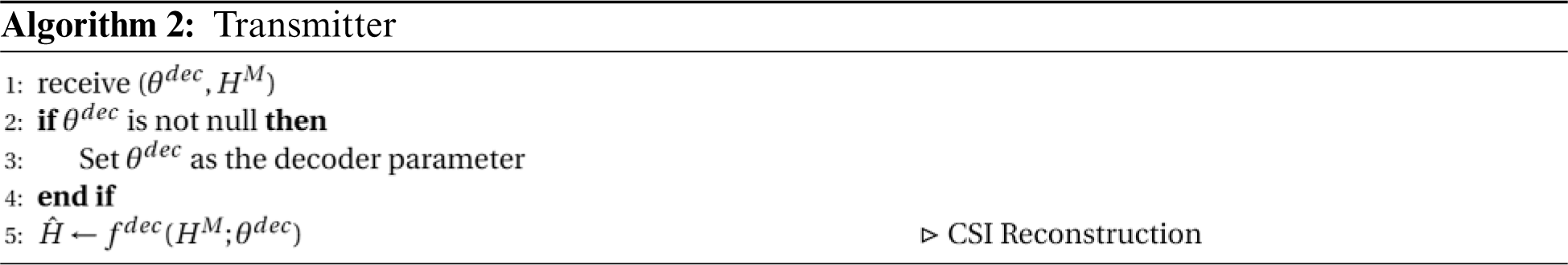
Every time the receiver compresses CSI, as a result of training, it obtains an optimization error, denoted as δ, which corresponds to the expected CSI recovery error at the transmitter. Depending on this value, it makes a decision about whether to send the decoder parameters to the transmitter or not. If a δ value is less than a predefined threshold, i.e., δthr, the receiver sends only the compressed CSI, i.e., HM, as this implies that the decoder parameters are still valid enough for the current target CSI thanks to the CSI prediction. Otherwise, the receiver obsoletes the previous decoder parameters; then, it re-trains the entire model and sends the newly trained decoder parameters (i.e., θdec) to the transmitter with the compressed CSI.

To summarize, we provide the entire proposed CSI feedback algorithm in Algorithms 1 and 2. Basically, the proposed method is designed for two communication entities, but it can be extended to multi-user scenarios as well. However, in this case, the transmitter may have to maintain different models for different users, which can cause additional operational burdens such as increased model sharing overhead. Therefore, we should consider mixing the proposed deep learning-based approach with traditional approaches. We leave this issue for our future work.

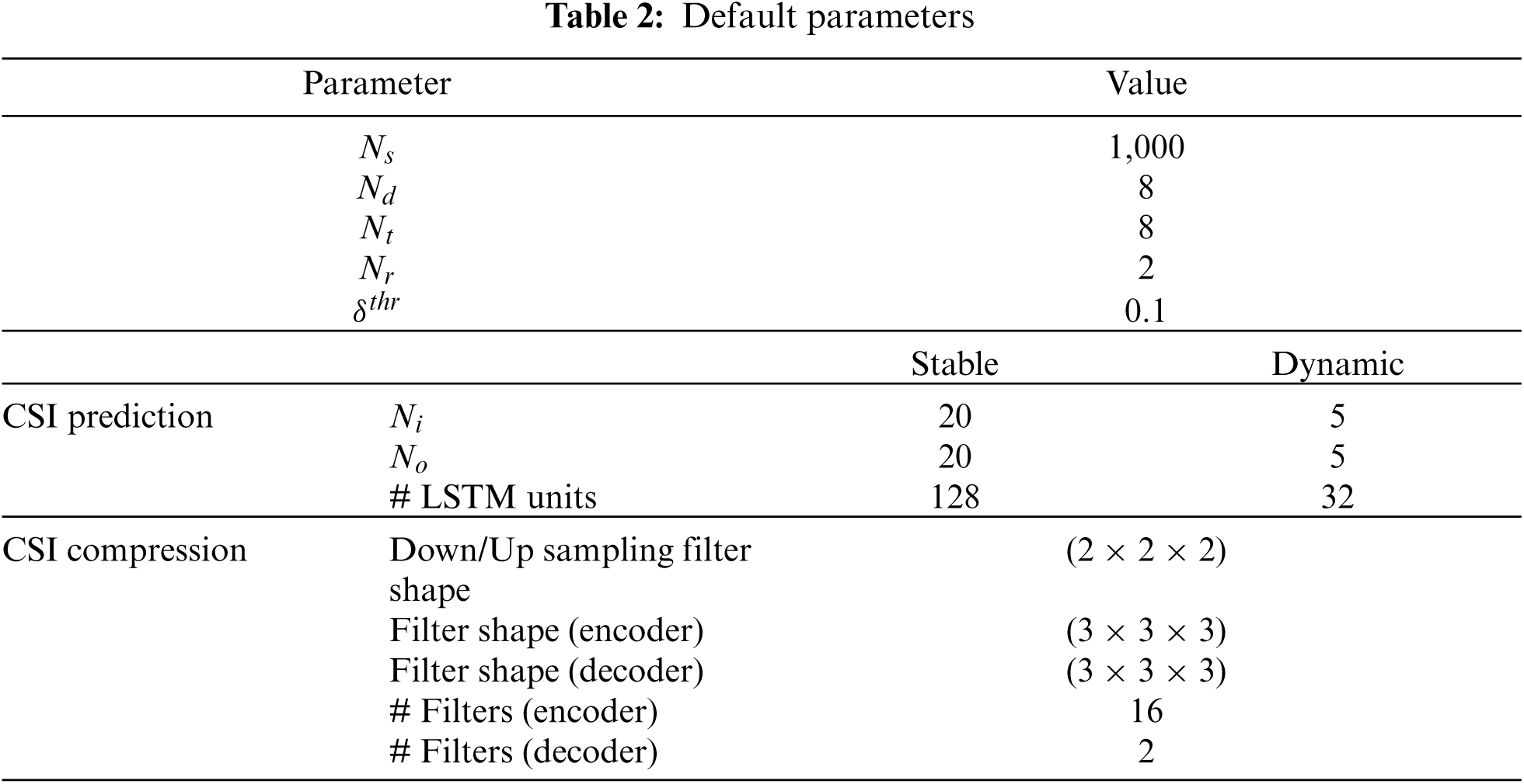
In this section, the performance of LCF is evaluated. We use TensorFlow 2 [26] to develop the proposed deep learning models of LCF and conduct extensive experiments on an Intel-i7 machine with 16 GB RAM and an NVIDIA RTX 3080 GPU. Using the MATLAB WINNER II model [27], we generate CSI datasets for both scenarios, which are sampled every 2 ms. When training the models, we use 70% of the total dataset for training, and the other 20% and 10% are used for validating and testing, respectively. For model optimization, we use the MSE as the objective, and employ Adam optimization [34] with a maximum of 1,000 epochs and a learning rate of 0.001. The default parameters used in the experiments are described in Tab. 2.

To compare the performance of LCF with those of other approaches, we additionally implement AFC [3] and CSINet [13]. Unfortunately, since all these schemes have different features and feedback policies, we have to make some modifications to them to ensure a fair comparison. The main changes are as follows:

• AFC: As AFC is not a machine learning-based approach, it does not require a training step and determines the degree of compression by calculating the expected compression error each time it receives CSI. The adaptive bit-quantization scheme is excluded since it can be applied to the other schemes as well. In the original AFC, the compression ratio can also be dynamically adjusted depending on the channel status, which is different from the other two schemes, which use a fixed compression ratio. In this study, for simplicity, we apply a fixed compression ratio to AFC.

• CSINet: CSINet considers only single-antenna receiver cases. In order to extend it to multi-antenna receiver cases, we repeatedly apply it to the channel of each receiving antenna. We use the same training configuration (both dataset and optimizer) for both CSINet and LCF.

• Both: All these schemes can skip a CSI transmission or model (i.e., decoder) parameter transmission if the expected CSI recovery error is less than δthr. Note that even if this condition is satisfied, LCF and CSINet should still send the compressed CSI to the transmitter.

Compression ratio α is defined as the ratio of the compressed data size to the original CSI data size (i.e., M2NdNtNr), and as a key performance metric, we measure the MSE, defined in the following equation [13]: MSE=||H−H^||2||H||2. In addition to the MSE, we use the cosine similarity between the original CSI and the reconstructed CSI to determine the value of δthr. The imperfect CSI due to the compression causes changes in the resulting beam steering vectors, which can be measured as the cosine similarity between the two CSI values [3,13]. Fig. 9 shows the cosine similarity values as a function of MSE for Nt=Nr=4 and Nd=16. To draw this plot, for each MSE value, we generate two sets of CSI matrices: One is randomly generated from the standard normal distribution, and the other is generated by adding random noise of the given MSE value to the previous matrix. After that, we compute the cosine similarity between the two matrices for each MSE value. The result is quite predictable; the cosine similarity decreases with the value of MSE. Based on this result, we set δthr as 0.1, where the cosine similarity is around 0.95.

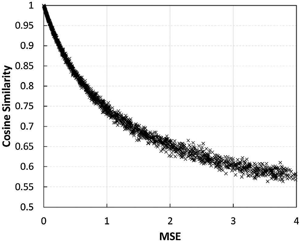
Figure 9: The same cosine similarity defined in CSINet [13] is used. We set the threshold for retraining as the point where the cosine similarity is around 0.95

In the following subsections, we first investigate the performance of each model used in LCF through micro-benchmarks, and then we compare the overall performance of LCF with those of the other approaches.

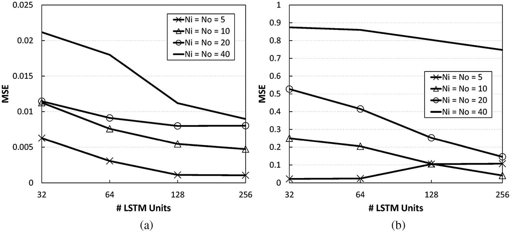
We investigate the impact of LSTM parameters on the prediction performance, according to varying numbers of LSTM units and different Ni and No combinations. Fig. 10 illustrates the plots of No=Ni cases for each scenario. It can be seen that the prediction accuracy decreases with the value of No, except for the case where No=5 and 256 units are used in the dynamic channel. This result is consistent with the previous observation shown in Fig. 7, where, as the model predicts CSI values for times farther in the future, the prediction error becomes larger.

Figure 10: CSI prediction performance for two channel cases, according to different numbers of LSTM units and Ni and No value combinations. In most cases, the prediction accuracy becomes better with more LSTM units and smaller Ni and No values. (a) Stable channel (b) Dynamic channel

The CSI prediction performance is mainly affected by the No value, but the number of LSTM units also has an effect. For all cases, the prediction becomes more accurate as the number of LSTM units increases, except for the No=5 case for the dynamic channel. This exception is due to the overfitting problem; using more LSTM units increases the model capacity too much, making it difficult to handle unobserved CSI data. Recall that in this evaluation, the dynamic channel has a relatively high and rapid channel variation compared to the stable one, and thus it is more likely to suffer from overfitting. Overall, better CSI prediction results are observed in the stable channel case than in the dynamic channel case; the worst MSE for the stable case is around 0.02, while for the dynamic case, it reaches almost 0.9. However, by taking small Ni and No values, we can improve CSI predictions in the dynamic channel as well; when No is 5 and the number of LSTM units is 32, the prediction error is at its lowest value of 0.02.

In this subsection, we evaluate the performance of the CSI compression model. To do this, for each scenario we first generate 20 CSI predictions with Ni=No=20 and use them to train the autoencoder. After that, we compress and restore the corresponding CSI label data with the trained model, measuring the difference between the two data. Recall that the decoder parameters are fixed once they are trained. We repeat this experiment 100 times and take the average value.

Fig. 11 shows the results in terms of the MSE and the number of decoder parameters, according to various numbers of encoder filters and compression ratios. First, from Figs. 11a and 11b, we can observe that the number of filters affects the compression performance greatly. For the same compression ratio, using more filters causes lower recovery errors. Unfortunately, in return for this high performance, the use of more filters causes the model to be larger, resulting in a high model sharing overhead, as shown in Fig. 11c. The number of filters is not the only factor to have an impact on the compression performance; the compression ratio affects the performance as well, since it directly affects the number of units in the fully connected layers of the autoencoder. As expected, the decoder size decreases with the compression ratio, at the expense of a high compression error. We also find that the recovery errors in the stable channel are overall lower than those in the dynamic channel, even though this difference is very subtle.

In this evaluation, we compare the performance of LCF with those of AFC [3] and CSINet [13]. We run each scheme for 20 consecutive CSI values and measure the average MSE and feedback size at different compression ratios from 1/8 to 1/128. Here, the feedback size is defined as the combined sizes of the model and the compressed CSI that are sent to the transmitter. We repeat this evaluation for both the stable and dynamic channel scenarios, and Fig. 12 shows the results.

From the results, we can see that AFC takes advantage of a small feedback size; for both scenarios, the maximum overhead is only 32, which is a much smaller number than those of other deep learning-based schemes. However, it suffers from high CSI recovery errors. As shown in Figs. 12a and 12d, its MSE values are all larger than 1, which is practically implausible. However, we note that the actual AFC can perform better than this modified AFC because of its adaptive compression ratio and quantization, which have been excluded in this evaluation. Compared to AFC, CSINet and LCF both have lower MSE results. When the compression ratio is 1/8, CSINet obtains minimum MSE values of 0.07 and 0.24 for both cases, respectively. Although these values are better than those of AFC, they still seem to be somewhat unstable. In particular, when using a higher compression ratio such as 1/128, or in a highly dynamic wireless channel scenario, the CSI recovery error increases significantly. Its MSE values are at around 0.5 in the dynamic case, as shown in Fig. 12d, which verifies our hypotheses that CSI compression would quickly become less effective without proper model updates. To make matters worse, this result eventually incurs a substantial model sharing overhead, as shown in Figs. 12b and 12e. The reason the two curves of the two scenarios show different patterns, i.e., one is going up while the other is going down, is because the major factor affecting the feedback size is different. In the stable channel case, model sharing rarely occurs at low compression ratios, and thus the feedback overhead decreases with the compression ratio; from Fig. 12c, we can see that only 1–2 model sharing transmissions happen when the compression ratio is lower than 1/32. However, using a higher compression ratio results in more frequent model sharing, causing the decoder size to take up most of the feedback overhead; as a result, when the compression ratio is 1/128, model feedback occurs for every CSI sample (Fig. 12c). Conversely, for the dynamic channel case, model sharing occurs for all CSI, as shown in Fig. 12f, so the number of model transmissions no longer has a significant impact on the results. In this case, the higher the compression ratio, the smaller the model size, which at the same time reduces the feedback overhead.

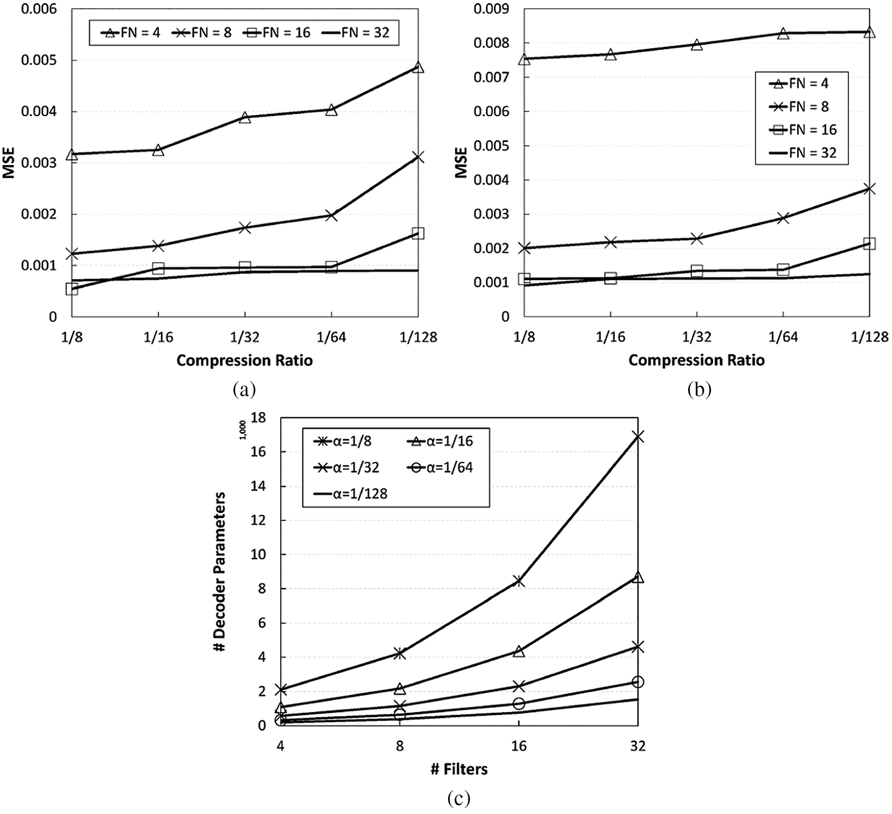
Figure 11: Impact of model parameters on the CSI compression model performance. For (a) and (b), ‘FN’ denotes the number of filters. In this evaluation, (3 × 2 × 3) filters are used, since the number of receiving antennas is two. (a) Recovery error (stable) (b) Recovery error (dynamic) (c) Decoder size

Overall, LCF outperforms the other approaches in terms of MSE. Even at the highest compression ratio of 1/128, it achieves an MSE value of 0.05, which is much lower than those of the other schemes. More surprisingly, LCF obtains this result with lower feedback overhead; the average feedback overhead values are only around 40 and 120, respectively, for both cases. From Fig. 12b, we can see that LCF has a higher feedback overhead than CSINet in the stable channel case when compression ratios are low (e.g., 1/8 and 1/16). This is due to the fact that LCF directly takes three-dimensional channel data as input, and thus the number of units in the fully connected layers is inherently larger than that of CSINet for the same compression ratio. As shown here, the gains of LCF may not be noticeable in these special situations, where model updates are not required much. However, in most cases, compared to the existing CSI feedback approaches, LCF obtains more stable and higher CSI compression performance, with only 10% of the model sharing overhead of the other approaches.

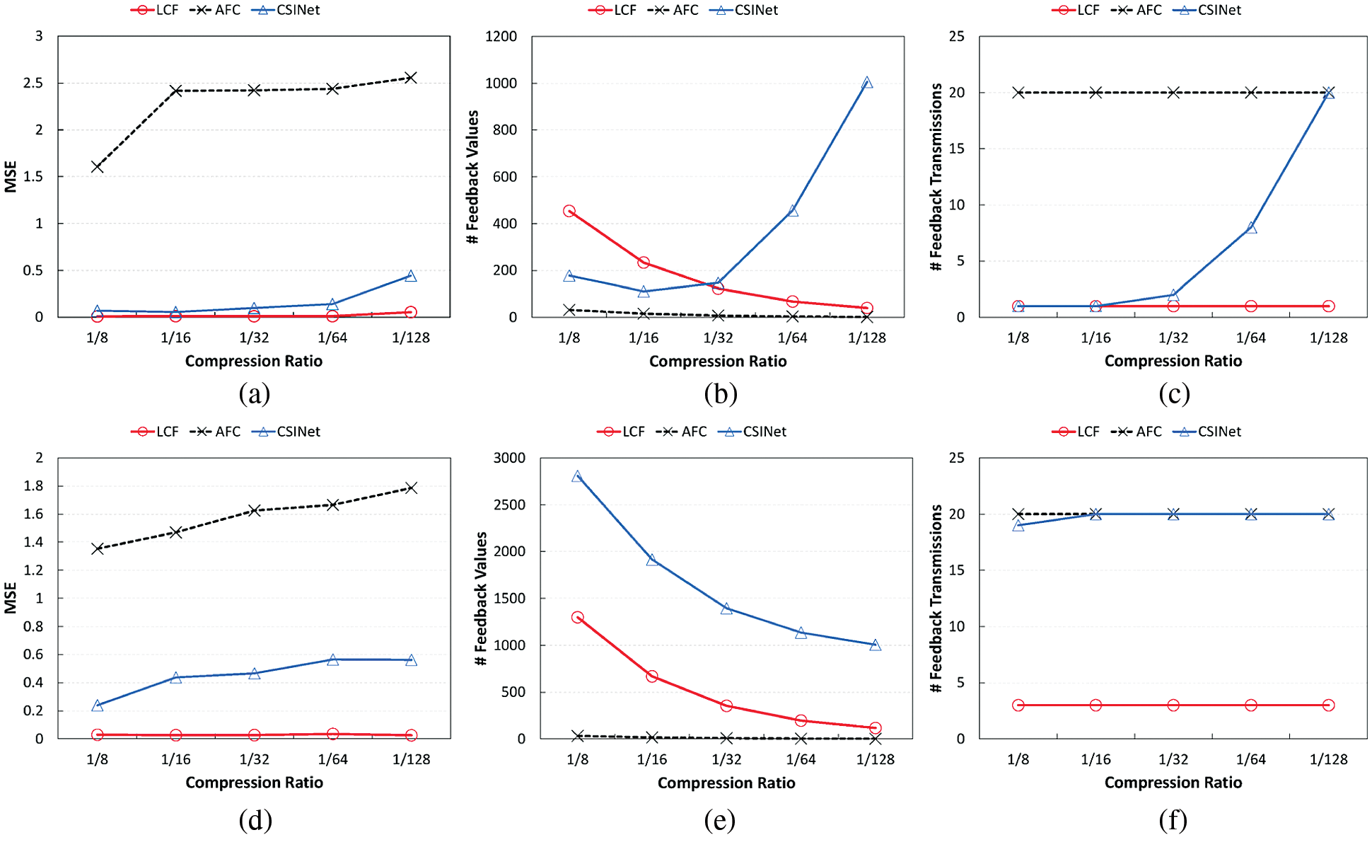
Figure 12: LCF outperforms AFC and CSINet in terms of MSE and feedback overhead. Even at the highest compression ratio of 1/128, it obtains much lower MSE values with lower feedback overhead. (a) Recovery error (stable) (b) Feedback size (stable) (c) # Feedback transmissions (stable) (d) Recovery error (dynamic) (e) Feedback size (dynamic) (f) # Feedback transmissions (dynamic)

In this paper, we propose LCF, which addresses the issues of conventional autoencoder-based CSI feedback schemes, specifically that CSI compression quickly becomes less effective and incurs an excessive model sharing overhead over time. Employing an autoregressive LSTM model, LCF generates CSI predictions and then exploits them to train the autoencoder, so that the compression model will be valid even for highly dynamic wireless channels. In order to fully capture the channel correlations to achieve higher CSI compression, three-dimensional convolutional layers are directly applied to the autoencoder. As a result, compared to the existing CSI feedback approaches, LCF obtains more stable and better CSI compression performance in terms of MSE, with only 10% of the model sharing overhead of the other approaches.

The LSTM model in LCF performs properly for forecasting time-series CSI data, but unfortunately it has the well-known drawback of a long training time. Several approaches can be considered to remedy this issue. First, instead of training the prediction model on all of the data, we can use an ensemble learning strategy that would update the model with the new data, and combine it with the existing model [35,36]. To overcome this limitation of LCF, we could also consider using a different type of network. Gated Recurrent Units (GRU) [37] could be one good alternative since it can take advantage of low computation with a smaller number of parameters compared to LSTM. Generally, Convolutional Neural Networks (CNNs) are computationally cheaper than the models in the Recurrent Neural Network (RNN) family, and thus they could be used for this task as well. In this case, it is easier to combine the two models of LCF, which are currently separated, into one model, resulting in higher efficiency. These schemes should be carefully considered not only with the two channel models currently used in this paper, but also with more realistic and diverse channel environments. We leave these issues for our future work.

Channel coherence time is defined as the point when the correlation value drops to 0.5 [33].

Funding Statement: This work was supported by the National Research Foundation of Korea (NRF) grant funded by the Korea government (MSIT) (No. 2021R1F1A1049778).

Conflicts of Interest: The authors declare that they have no conflicts of interest to report regarding the present study.

References

3GPP, “MU-MIMO-3GPP specifications,” 3GPP TR V16, 202 [Online]. Available: http://www.3gpp.org/DynaReport/FeatureOrStudyItemFile-470012.htm.
IEEE80org, “8011ax,” IEEE 8011 HEW SG Meeting, 2014. [Online]. Available: http://www.ieee80org/11/Reports/hew_update.htm.
X. Xie, X. Zhang and K. Sundaresan, “Adaptive feedback compression for MIMO networks,” in Proc. the 19th Annual Int. Conf. on Mobile Computing & Networking, New York, NY, USA, pp. 477–488, 201
C. Shepard, H. Yu, N. Anand, E. Li, T. Marzetta et al., “Argos: Practical many-antenna base stations,” in Proc. the 18th Annual Int. Conf. on Mobile Computing and Networking, New York, NY, USA, pp. 53–64, 2012.
Q. Yang, X. Li, H. Yao, J. Fang, K. Tan et al., “Bigstation: Enabling scalable real-time signal processing in large mu-mimo systems,” in Proc. the ACM SIGCOMM 2013 Conf. on SIGCOMM, Hong Kong, China, pp. 399–410, 2013.
X. Xie and X. Zhang, “Scalable user selection for MU-MIMO networks,” in Proc. IEEE Conf. on Computer Communications, Toronto, ON, Canada, pp. 808–816, 2014.
T. Yoo and A. Goldsmith, “Optimality of zero-forcing beamforming with multiuser diversity,” in Proc. IEEE Int. Conf. on Communications, Seoul, Korea, pp. 542–546, 2005.
K. Huang, R. W. Heath and J. G. Andrews, “Limited feedback beamforming over temporally-correlated channels,” IEEE Transactions on Signal Processing, vol. 57, no. 5, pp. 1959–1975, 2009.
X. Sun, L. J. Cimini, L. J. Greenstein, D. S. Chan and B. Douglas, “Performance of quantized feedback beamforming in MIMO-OFDM links over time-varying, frequency-selective channels,” in Proc. IEEE Military Communications Conf., Orlando, FL, USA, pp. 1–6, 2007.
Z. Gao, L. Dai, Z. Lu, C. Yuen and Z. Wang, “Super-resolution sparse MIMO-OFDM channel estimation based on spatial and temporal correlations,” IEEE Communications Letters, vol. 18, no. 7, pp. 1266–1269, 2014.
M. Ozdemir, E. Arvas and H. Arslan, “Dynamics of spatial correlation and implications on MIMO systems,” IEEE Communications Magazine, vol. 42, no. 6, pp. 14–19, 2004.
U. Karabulut, A. Awada, I. Viering, M. Simsek and G. P. Fettweis, “Spatial and temporal channel characteristics of 5G 3D channel model with beamforming for user mobility investigations,” IEEE Communications Magazine, vol. 56, no. 12, pp. 38–45, 2018.
C. K. Wen, W. T. Shih and S. Jin, “Deep learning for massive MIMO CSI feedback,” IEEE Wireless Communications Letters, vol. 7, no. 5, pp. 748–751, 2018.
Z. Liu, L. Zhang and Z. Ding, “An efficient deep learning framework for low rate massive MIMO CSI reporting,” IEEE Transactions on Communications, vol. 68, no. 8, pp. 4761–4772, 2020.
C. Lu, W. Xu, H. Shen, J. Zhu and K. Wang, “MIMO channel information feedback using deep recurrent network,” IEEE Communications Letters, vol. 23, no. 1, pp. 188–191, 2019.
T. Wang, C. K. Wen, S. Jin and G. Y. Li, “Deep learning-based CSI feedback approach for time-varying massive MIMO channels,” IEEE Wireless Communications Letters, vol. 8, no. 2, pp. 416–419, 2019.
M. Hussien, K. K. Nguyen and M. Cheriet, “PRVNet: Variational autoencoders for massive MIMO CSI feedback,” arXiv preprint arXiv:2011.04178. 2020.
Z. Liu, L. Zhang and Z. Ding, “Exploiting bi-directional channel reciprocity in deep learning for low rate massive MIMO CSI feedback,” IEEE Wireless Communications Letters, vol. 8, no. 3, pp. 889–892, 2019.
T. J. O'Shea, T. Erpek and T. C. Clancy, “Deep learning based MIMO communications,” arXiv preprint arXiv:1707.07980. 2017.
D. J. Ji, J. Park and D. H. Cho, “ConvAE: A new channel autoencoder based on convolutional layers and residual connections,” IEEE Communications Letters, vol. 23, no. 10, pp. 1769–1772, 2019.
D. J. Ji and D. H. Cho, “ConvAE-Advanced: Adaptive transmission across multiple timeslots for error resilient operation,” IEEE Communications Letters, vol. 24, no. 9, pp. 1976–1980, 2020.
H. He, C. K. Wen, S. Jin and G. Y. Li, “Deep learning-based channel estimation for beamspace mmWave massive MIMO systems,” IEEE Wireless Communications Letters, vol. 7, no. 5, pp. 852–855, 2018.
J. M. Kang, C. J. Chun and I. M. Kim, “Deep-learning-based channel estimation for wireless energy transfer,” IEEE Communications Letters, vol. 22, no. 11, pp. 2310–2313, 2018.
C. A. Metzler, A. Maleki and R. G. Baraniuk, “From denoising to compressed sensing,” IEEE Transactions on Information Theory, vol. 62, no. 9, pp. 5117–5144, 2016.
D. L. Donoho, A. Maleki and A. Montanari, “Message passing algorithms for compressed sensing,” Proceedings of the National Academy of Sciences, vol. 106, no. 45, pp. 18914–18919, 2009.
Google, “Tensorflow 2.0.,” 2021. [Online]. Available: https://www.tensorflow.org/.
Mathworks, “WINNER II channel model for MATLAB communications toolbox,” 2021. [Online]. Available: https://www.mathworks.com/matlabcentral/fileexchange/59690-winner-ii-channel-model-for-communications-toolbox.
J. Meinilä, P. Kyösti, T. Jämsä and L. Hentilä, “WINNER II channel models,” Radio Technologies and Concepts for IMT-Advanced, pp. 39–92, 2009.
M. Series, “Guidelines for evaluation of radio interface technologies for IMT-advanced,” Report ITU, vol. 638, pp. 1–72, 2009.
F. Ademaj, M. Taranetz and M. Rupp, “3GPP 3D MIMO channel model: A holistic implementation guideline for open source simulation tools,” EURASIP Journal on Wireless Communications and Networking, vol. 2016, no. 1, pp. 1–14, 2016.
A. Karttunen, J. Jarvelainen, A. Khatun and K. Haneda, “Radio propagation measurements and WINNER II parameterization for a shopping mall at 60 GHz,” in Proc. IEEE 81st Vehicular Technology Conf., Glasgow, UK, pp. 1–5, 2015.
G. Breit, “Coherence time measurement for TGac channel model,” IEEE 802.11-09/1173r1, pp. 1–16, 2009.
D. Tse and P. Viswanath, Fundamentals of Wireless Communication. Cambridge, England: Cambridge University Press, 2005.
D. P. Kingma and J. Ba, “Adam: A method for stochastic optimization,” arXiv preprint arXiv:1412.6980. 2014.
L. Rokach, “Ensemble-based classifiers,” Artificial Intelligence Review, vol. 33, no. 1, pp. 1–39, 2010.
A. Wasay, B. Hentschel, Y. Liao, S. Chen and S. Idreos, “Mothernets: Rapid deep ensemble learning,” Proceedings of Machine Learning and Systems, vol. 2, pp. 199–215, 2020.
K. Cho, B. van Merrienboer, Ç. Gülçehre, F. Bougares, H. Schwenk et al., “Learning phrase representations using RNN encoder-decoder for statistical machine translation,” arXiv preprint arXiv:1406.1078. 2014.

Computers, Materials & Continua DOI:10.32604/cmc.2022.024562
Article