DOI:10.32604/cmc.2022.024535
| Computers, Materials & Continua DOI:10.32604/cmc.2022.024535 | |
| Article |
Examination of Pine Wilt Epidemic Model through Efficient Algorithm
1Department of Mathematics, Govt. Maulana Zafar Ali Khan Graduate College Wazirabad, Punjab Higher Education Department (PHED), Lahore, 54000, Pakistan
2Department of Mathematics, College of Science, Taif University, Taif, 21944, Saudi Arabia
3Department of Mathematics, Cankaya University, Balgat, Ankara, 06530, Turkey
4Department of Medical Research, China Medical University, Taichung, 40402, Taiwan
5Department of Mathematics, Faculty of Sciences, University of Central Punjab, Lahore, 54600, Pakistan
6Department of Mathematics, Technische Universitat Chemnitz, 6209111, Germany
7Department of Mathematics and Statistics, King Faisal University, Al Ahsa, 31982, Saudi Arabia
*Corresponding Author: Ali Raza. Email: alimustasamcheema@gmail.com
Received: 21 October 2021; Accepted: 22 November 2021
Abstract: Pine wilt is a dramatic disease that kills infected trees within a few weeks to a few months. The cause is the pathogen Pinewood Nematode. Most plant-parasitic nematodes are attached to plant roots, but pinewood nematodes are found in the tops of trees. Nematodes kill the tree by feeding the cells around the resin ducts. The modeling of a pine wilt disease is based on six compartments, including three for plants (susceptible trees, exposed trees, and infected trees) and the other for the beetles (susceptible beetles, exposed beetles, and infected beetles). The deterministic modeling, along with subpopulations, is based on Law of mass action. The stability of the model along with equilibria is studied rigorously. The authentication of analytical results is examined through well-known computer methods like Non-standard finite difference (NSFD) and the model's feasible properties (positivity, boundedness, and dynamical consistency). In the end, comparison analysis shows the effectiveness of the NSFD algorithm.
Keywords: Pine wilt disease; modeling; NSFD algorithm; linearization of NSFD algorithm; results
Pine wilt disease (PWD), a severe disease produced by the pinewood worm that affects regularly planted pines, disrupts ecosystems and destroys biodiversity. Symptoms of PWD usually seem in late spring or early summer. The lack of resin exudation from bark wounds is the most evident indication. At this time, the tree succumbs to the disease and dies. The trees that are affected lose all of their resin, and their wood turns dry. From both an economic and an environmental (landscape) standpoint, it poses a significant threat to forest ecosystems worldwide. Pine trees get infected with PWD, which causes them to wilt, and the tree goes to the death phase within a few months. The absence of resin exudation from bark wounds is the first apparent symptom. Long-horned pine sawyer beetles transport pinewood nematodes from diseased trees to healthy or infected pines. The disease is spread from one pine tree to another by the pine sawyer, a bark beetle that feeds on the bark and phloem of susceptible live tree twigs, or female beetles laying eggs in newly cut timber or dead trees. If conditions are suitable for disease development, nematodes during “primary transmission” can spread quickly in the sapwood. If the beetle carries the pinewood nematode, it might apply to new trees. Pines are growing well in sharp muds, and some are also growing well enough in calcareous soils. The pine wilt disease has gradually spread to warm, modest places, and the average annual temperature has topped 10°C. For pine wilt to grow and blow out, several months of warm, dry conditions are required. The roundworm was first discovered in longleaf pine wood in Louisiana, United States. Infection and nematode completion of pines begin in June or July, but no visible symptoms develop until late summer or fall. While the discase growths needles go from deadly green to dark and finally brunet due to a lack of water due to the critical water plan being squashed, the spines first and foremost discolor sea green. Still, they do not wait or become loose as is combined for broadleaf trees affected by wilt diseases. More than the cold, the tree's unmoving needles remain attached to it. Many gums are frequently associated with physical wounds or injuries caused by cockroaches. Pine wilt virus is a severe disease caused by roundworms that pine sawyer beetles spread. Any condition that disrupts the vascular structure of floras is referred to as a wit disease. Fungi, bacteria, and nematodes can quickly kill plant life, including massive branches and entire trees. Pine wilt kills trees and leaves a blue stain on the wood. The only technique for recognizing pine wit is sending a wood representation to an experimental laboratory for worm removal and approval. Pathologists usually require a wood replica from the stalk or a loose branch. The speculum is compacted into a round-shaped at the landfill, the observable vulvar boundary is lap-like, and the concluding phases of the feminine are rounded in Bursaphelenchus xylophilus. The pine wilt roundworm has a complex life cycle, with quarter-developed stages and an older location that reproduces sexually by reciprocal male and female reproduction. The microphagous phase of the life cycle occurs in decaying or dead wood when roundworms live and feed on mushrooms rather than the wood itself. In the past, the roundworm pathogen was known as Monochamus alternates sawyer insect, and it was one of the experimental pests due to the widespread death of pine trees. Infection with pine wilt is a disease that affects poisonous pine plants. More or less diseased trees serve as inactive transporters that have been dormant for a year or more and cannot detect observable symbols. While vector-borne diseases are more well-known in humans, they are also prevalent in floras. Some of the most severe flaccid conditions of trees, including pine wilt and palm red ring disease, are caused by roundworms, which have a fascinating relationship with insect vectors. Pesticides applied to foliar are ineffective in preventing pine wilt. On the other hand, preventive nematicide systemic inoculations are a successful but costly control method. Pathogens that cause wilting diseases target vascular vessels and cause the xylem to flop to carry water to the foliage, causing stalks and greeneries to wilt. Plant nematicide and pesticide management have been determined to be economically impossible, if not unsuccessful, in the United States. Therapeutic supporters after indications have appeared, in distinction, to be ineffective. Pesticides applied to foliar are ineffective in preventing pine wilt. However, universal preventative boosters of nematicides constitute an active but costly control strategy. The best approach to avoiding pine wilt is to keep your trees healthy and strong by watering them during dry seasons. Stress trees are attracting the attention of beetles. Pine is useful for swelling (redness) in the upper and lower respiratory areas, a runny nose, roughness, a common cold, coughing or bronchitis, high temperatures, a contagious inclination, and blood pressure issues. For mild muscle and nerve discomfort, some people apply pine directly to the skin. Pine needle drink also contains a lot of vitamin A, which is helpful for your eyesight, hair and skin regrowth, and red blood cell production. It can be used as a cough syrup to treat coughs and rib congestion and for sore throats. Mathematical modeling is a powerful tool for describing how the disease spreads. We can regulate those components that substantially impact the disease's transmission, and we can prepare several control measures to limit contamination's spread. Haq et al. [1] in 2017, presented a fractional-order wide-ranging model designed for the blowout of pine wilt disease using the Laplace Adomian decomposition method. Ozair et al. [2] in 2020, proposed a vector-swarm scientific model for the pine wilt disease taking local sensitivity analysis of parameters and numerical experiments to illustrate the theoretical bases for the anticipation and governor of the disease. Khan et al. [3] in 2017, suggested a mathematical classification of calculations for the pine wilt disease in two ways. Abodayeh et al. [4] in 2020, established a mathematical model to explore the result of an asymptomatic carrier to identify critical parameters to examine several intervention options. Lee investigated the best controller approach for anticipating pine wilt disease using analytical and numerical techniques acceptable to do; we put on two control approaches; tree-injecting of nematicides and the destruction of adult beetles through floating pesticide spraying [5]. Khan et al. [6] in 2018, presented the Caputo-Fabrizio fractional-order mathematical model of pine wilt disease to investigate elementary properties of the model also check numerical simulation by taking a particular parameter. Agarwal et al. in 2019, recommended a stochastic pine wilt disease model taking the primary reproductive number, and an adequate condition is provided to study the extinction and permanence of the disease. Underlying the stochastic differential equation system is analyzed, and proper Lyapunov functionals are formulated to show the stability analysis [7]. Awan et al. [8] in 2018, recommended qualitative research and sensitivity-based model taking reproduction numbers in the specific form to check the result of three control measures. Tamura et al. in 2019, proposed spatiotemporal analysis of pine wilt disease using the quantified number of PWNs and face levels of supposed pathogenesis-related (PR) genes in different positions of Japanese black pine seedling over time cured by Taqman quantitative real-time PCR (qPCR) assay. As a result, PWNs and PR levels increased drastically, leading to plant death [9]. Hirata et al. in 2017, explored the potential distribution of PWD under climate change scenarios. Pinus forests are at risk of serious harm due to environmental shifts and the spread of PWD [10]. Lee et al. [11] in 2013, studied a disease transmission model based on primary reproduction number Ro. If Ro is a smaller amount than one than disease-free equilibrium state obtained if Ro more than one then endemic equilibrium is globally asymptotically stable condition obtained. Shah et al. [12] in 2018, suggested swarm vector dynamics of pine wilt disease model taking worldwide asymptotic constancy investigation at changed equilibrium points and exposed that disease vanishes when beginning quantity falls less unity. Awan et al. [13] in 2016, studied the qualitative behavior of pine wilt disease by considering indirect and direct transmission using primary reproduction numbers. Gao et al. in 2015, studied pine wilt disease attacks happening earth possessions and pine woodland groups in the three valleys region of China. This study shows that the PWD has stuck Masson pine forest soil properties and altered forest communal structure. The disease is negatively related to Masson pine and positively associated with broad-leaved trees [14]. Shi et al. in 2013, proposed a scientific model for the spread of pine wilt disease. Primary reproduction numbers determine the global dynamics [15]. Nguyan et al. in 2016, recommended a spatially explicit model of pine wilt disease taking dispersal pattern (direction and area) of Asia such as infested neighborhoods, short- and long-distance dispersal, asymptomatic carriers, and typhoon (incorporating biological and environmental events). Using receiver operating characteristics and pair-correlation functions shows that disease occurs in both local and global aspects [16]. Khan et al. [17] in 2018, studied the changing elements of pine wilt disease is stable happening local and globally. Hussain et al. [18] investigated the dynamics of pine wilt disease with the sensitivity of parameters. Raza et al. [19] studied the structure-preserving analysis of the epidemic model with necessary properties. Some more techniques related to epidemic models are presented in [20,21]. The well-known results with different techniques are studied in [22,23]. For the best presentation, more work on the epidemiology and efficiency of the techniques are studied in [24–32]. In this paper, we study the dynamics of pine wilt disease via algorithms. We can observe that computational methods in literature have many problems like negativity, unboundedness, and inconsistency of solutions. These issues will resolve by our proposed idea that is a non-standard finite difference method (NSFD). Also, NSFD fulfills the properties of the biological problem. The rest of the paper is styled as follows: In Section 2, the modeling of pine wilt disease is defined. In Section 3, the construction ways of the epidemic model, equilibrium points, and computational methods and their convergence. In the last section conclusion and future problems are discussed.
2 Modelling of Pine Wilt Disease
These are the various symbols. Six-of them are used as variables, and the remaining are all parameters. Both types of notations describe the given epidemic model.
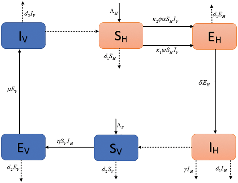
Figure 1: Flow map of pine wilt disease
The fixed values of the model is defined as follows:
With nonnegative conditions
The system (1–6) has two types of equilibria in the feasible region
Disease-free equilibrium
Endemic equilibrium = (SH*, EH*, IH*, SV*, EH*, IH*)
In this section, we find the reproduction number Ro by using the next-generation method. We introduce two types of matrices: the transition matrix and the second is transmission matrix.
Here,
Theorem 1: (Local stability) Forgiven
Proof: Let us consider,
Therefore, model (1–6) will be converted into a new form
The general Jacobian matrix is defined as
By substituting the values, we obtained
At the disease-free point
Here we let
Clearly,
This implies that disease-free point K0 is locally Asymptotically stable.
Theorem 2: Forgiven
Proof: The given Jacobean matrix at Endemic equilibrium (EE)
The characteristic polynomial equation attached with
where
Here, we have
The polynomial Eq. (2.7) has the Routh-Hurwitz criteria presented as follows:
When R0 is greater than 1, the characteristic Eq. (7) has eigenvalues with negative real parts if
3 Non-Standard Finite-Difference Algorithm
The NSFD could be developed for the system (1)–(6), the Eq. (1) of the pine wilt epidemic model may be calculated as:
The decomposition of proposed method is as follows:
In the same way, we decompose the remaining system into proposed NSFD method, like (9), as follows:
where the discretization gap is denoted by “h”.
3.1 Linearization Process of NSFD Algorithm
In this section, we shall present the theorem at the equilibrium of the model for the process of linearization of the NSFD algorithm is as follows:
Theorem 3: The NSFD algorithm is stable if the eigenvalues of Eqs. (9)–(14) lie in the same unit circle for any
Proof: Consider the right-hand sides of the equation in (9–3.14) as functions F, G, H, J, K, L
The general from of Jacobian matrix, we have
The given Jacobean matrix at Disease-Free Equilibrium (DFE)
Now, for endemic equilibrium (EE) K1= (SH*, EH*, IH*, SV*, EV*, IV*). The given Jacobean matrix is
The proof is straightforward. By using the Mathematica, this is a guarantee to the fact that all values of Jacobian lie in a unit circle, as desired.
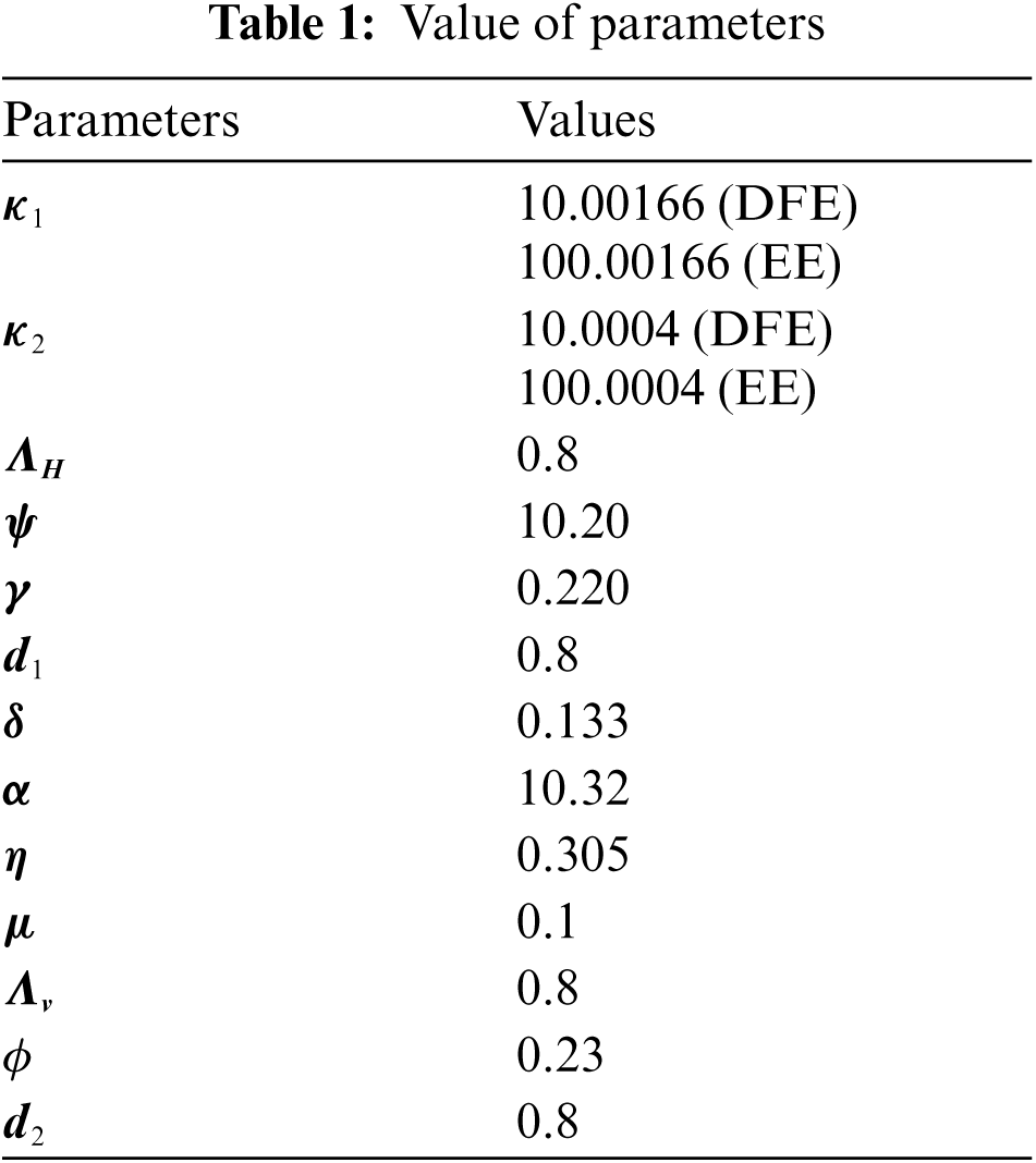
In this section, we used the scientific literature presented in Tab. 1 for the simulating behavior of the system (9)–(14) at both equilibria of the model as follows:
4 Results and Concluding Remarks
Fig. 2 depicts the transmission map of disease via bar chart. Fig. 3 shows that the two-dimensional kernel density between years and its transmission. Fig. 4 shows the distribution analysis of illness at the given data. Fig. 5 shows the splines connectedness of disease. In Figs. 6a–6b, we used the command-built software ODE-45 to simulate the model's behavior at any time t. In Figs. 7a–7b, is the true sense results affected by the non-standard finite difference method at any time step size. This computer method has the advantage over the other two methods like Euler and Runge Kutta. Independent of time step size, low-cost and effective technique.
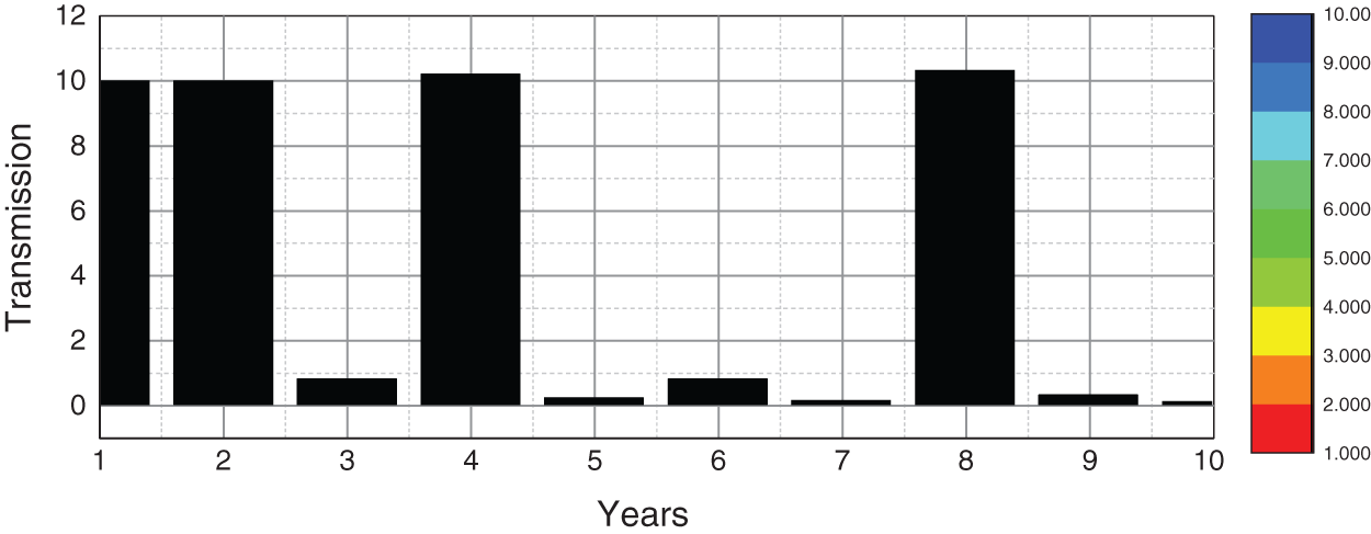
Figure 2: Transmission map of pine wilt disease
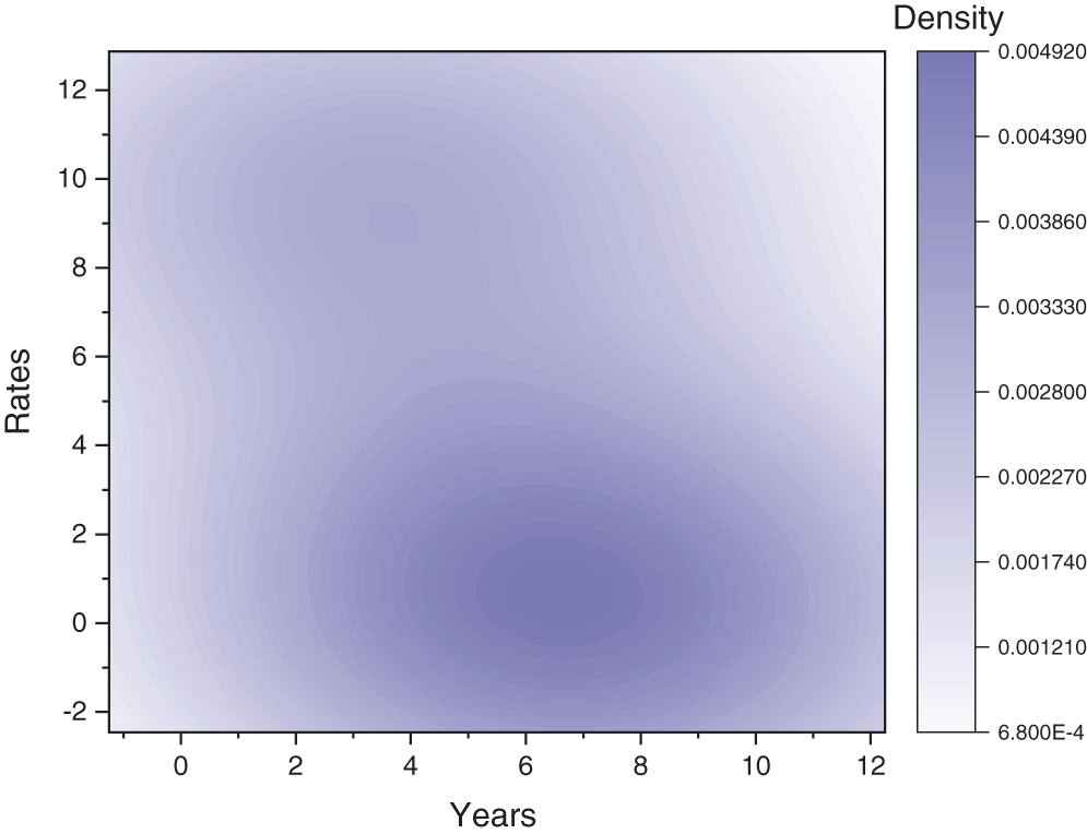
Figure 3: Two-dimensional kernel density
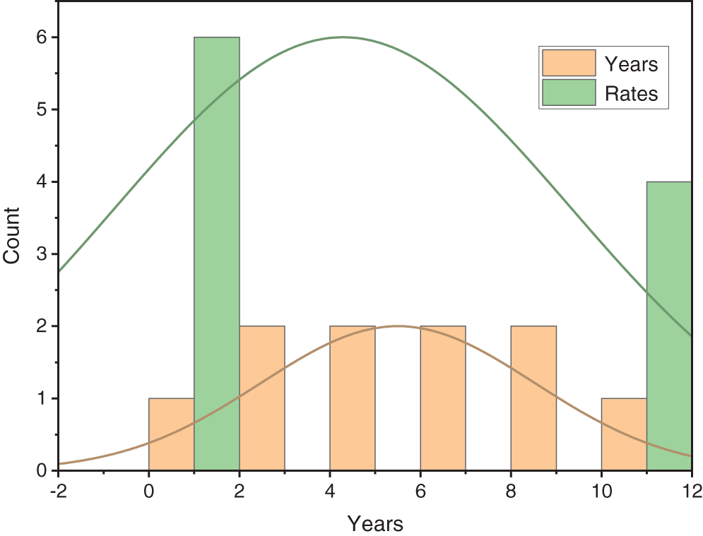
Figure 4: Distribution analysis of disease
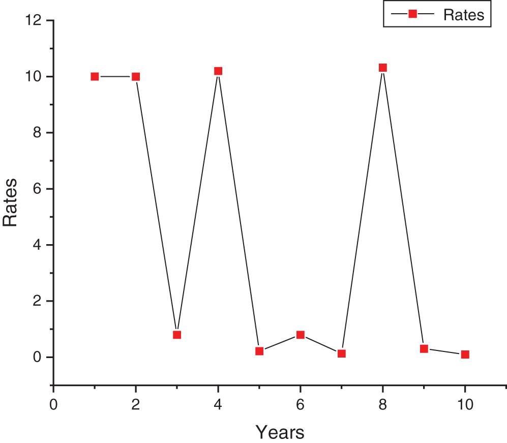
Figure 5: Spline connectivity of disease rates
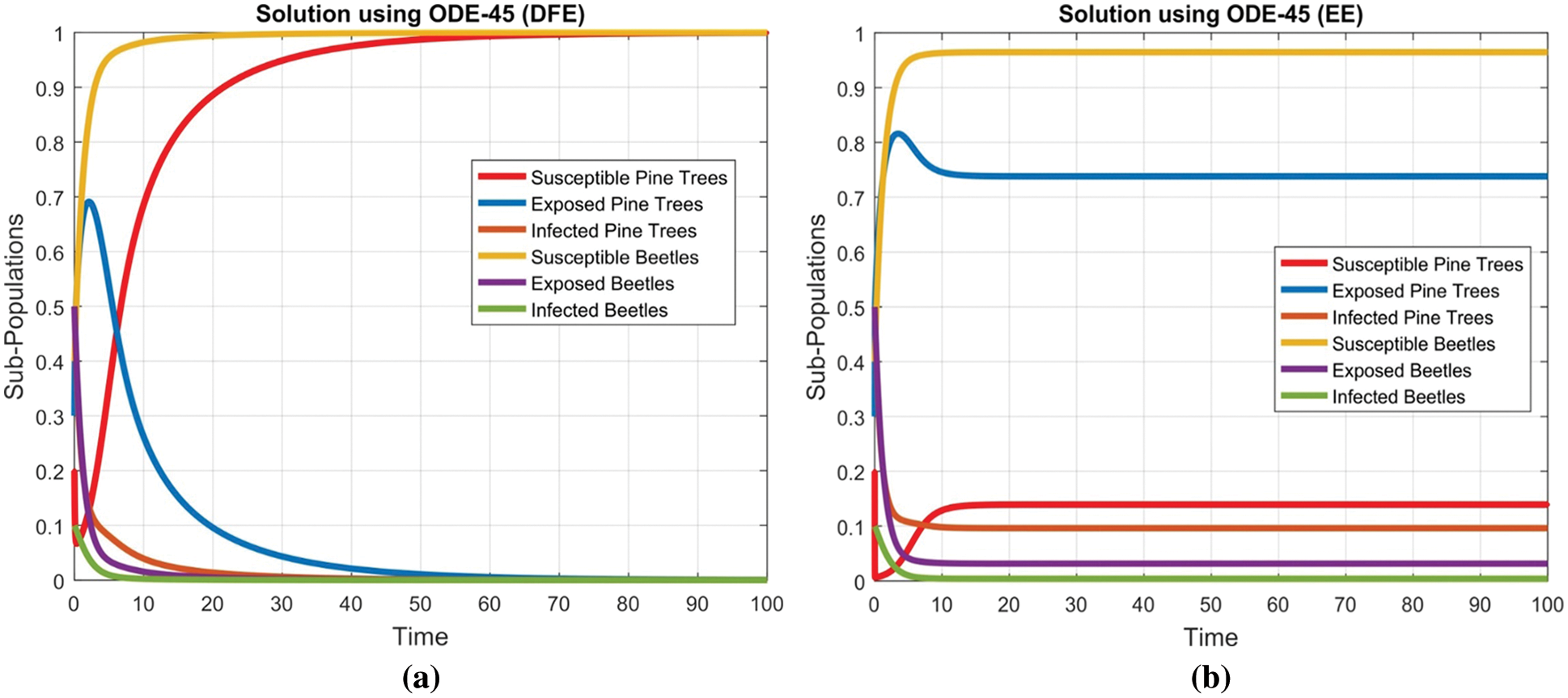
Figure 6: Combined graphical behavior for the equilibria and converges at time t (a) sub-populations at disease-free equilibrium (b) Sub-populations at endemic equilibrium
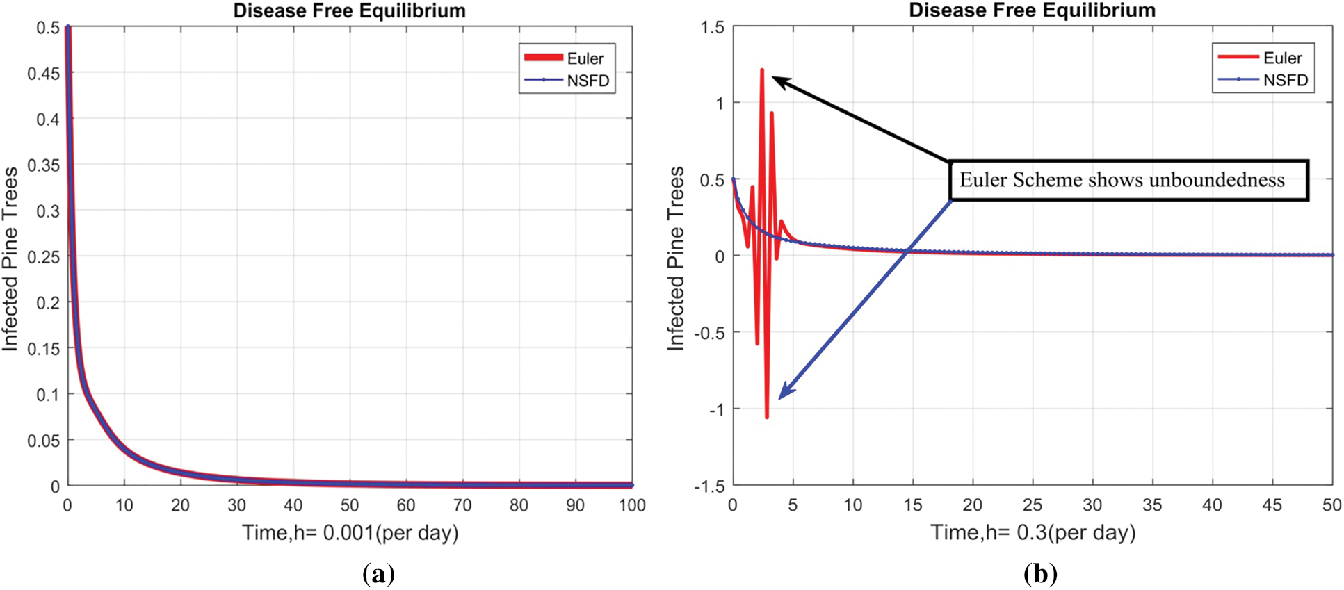
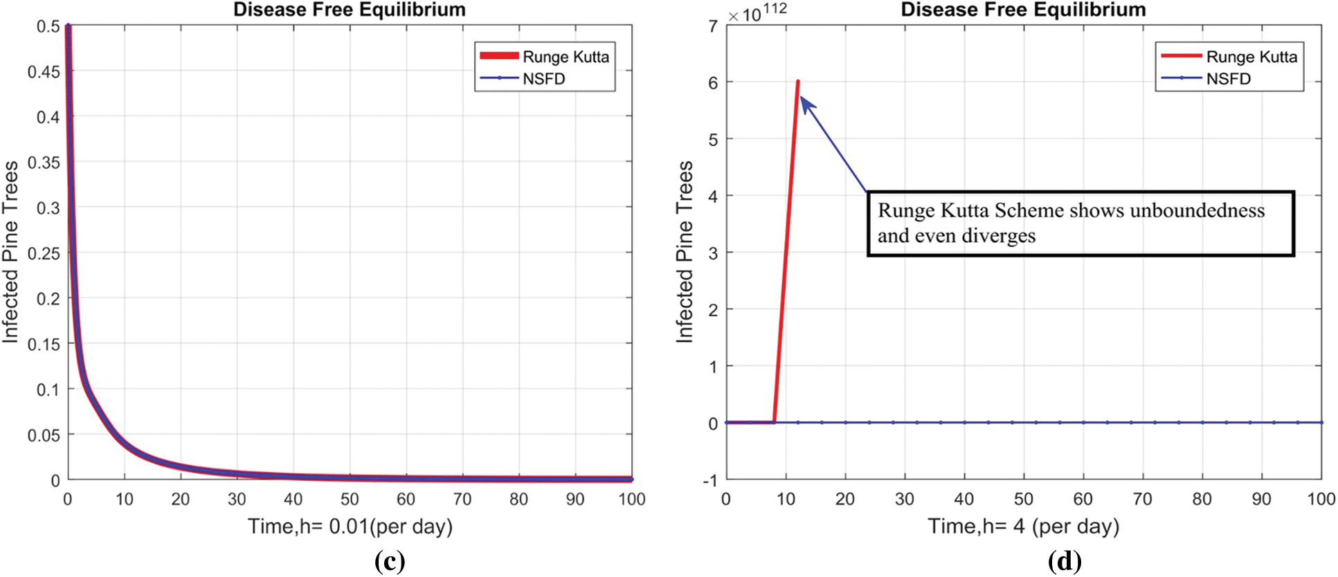
Figure 7: Combined behaviors of NSFD with Euler and Runge Kutta at different step sizes (a) Combine behavior at DFE when h = 0.001 (b) (Divergent) Combine behavior at DFE when h = 0.3 (c) Combine behavior at DFE when h = 0.01. (d) (Divergent) Combine behavior at DFE when h = 4
In this article, we investigated the subtleties of the numerical epidemic model with numerical strategies’ effective use. We divided the entire tree population into six groups: susceptible trees, exposed trees, infected trees, easy vector beetles, exposed vector beetles, and infected vector beetles. We have calculated the reproduction number for the pine wilt disease numerical epidemic model. We have also presented the local stability at the steady states of the model, that is, at pine wilt free equilibrium and at pine wilt existing compensation, by using well-known mathematics results. We have concluded that we can control the dynamic of the pine wilt by positively using different affected techniques like, vaccination is proved to be the ultimate solution to avoid the spread of this disease. Immunization is much essential and is recommended for trees that fall under this disease.
Moreover, Booster doses are recommended for disease trees to make sure of vaccination. And most importantly, a sound hygiene system is much needed to adapt, which can play a vital role in reducing the spread of pine wilt disease. In the future, we could extend this type of modeling to other complex epidemiological models and their branches.
Acknowledgement: Thanks, our families and colleagues who supported us morally.
Funding Statement: The authors received no specific funding for this study.
Conflicts of Interest: The authors declare that they have no conflicts of interest to report regarding the present study.
1. L. F. Haq, K. Shah and M. Shahzad, “Numerical analysis of fractional-order pine wilt disease model with bilinear incident rate,” Journal of Mathematics and Computer Science, vol. 17, no. 1, pp. 420–428, 2017. [Google Scholar]
2. M. Ozair and J. P. Leiton, “Analysis of a mathematical model for the pine wilt disease using a graph-theoretic approach,” Applied Science, vol. 22, no. 1, pp. 189–204, 2020. [Google Scholar]
3. M. A. Khan, K. Ali, E. Bonyah, K. O. Okosun, S. Islam et al., “Mathematical modelling and stability analysis of pine wilt disease with optimal control,” Scientific Reports, vol. 7, no. 1, pp. 1–19, 2017. [Google Scholar]
4. K. Abodayeh, A. Raza, M. S. Arif, M. Rafiq, M. Bibi et al., “Stochastic numerical analysis for impact of heavy alcohol consumption on transmission dynamics of gonorrhoea epidemic,” Computers Materials and Continua, vol. 62, no. 3, pp. 1125–1142, 2020. [Google Scholar]
5. K. S. Lee, “Stability analysis and optimal control strategy for prevention of pine wilt disease,” Abstract and Applied Analysis, vol. 14, no. 1, pp. 1–15, 2014. [Google Scholar]
6. M. A. Khan, S. Ullah, K. O. Okosun and K. Shah, “A Fractional-order pine wilt disease model with caputo-fabrizio derivative,” Advance in Difference Equation, vol. 410, no. 1, pp. 1–18, 2018. [Google Scholar]
7. R. P. Agarwal, Q. Badshah, G. Rahman and S. Islam, “Optimal control and dynamical aspects of a stochastic pine wilt disease model,” Journal of the Franklin Institute, vol. 356, no. 1, pp. 3991–4025, 2019. [Google Scholar]
8. A. U. Awan, T. Hussain, K. O. Okosun and M. Ozair, “Qualitative analysis and sensitivity based optimal control of pine wilt disease,” Advance in Difference Equation, vol. 27, no. 1, pp. 1–19, 2018. [Google Scholar]
9. M. Tamura, R. Yamagachi, K. Matsunaga and T. Hirao, “Spatiotemporal analysis of pine wilt disease: Relationship between pinewood nematode distribution and defence response in pinus thunbergii seedlings,” Forest Pathology, vol. 49, no. 1, pp. 1–9, 2019. [Google Scholar]
10. A. Hirata, K. Nakamura, K. Nakao, Y. Kominami, N. Tanaka et al., “Potential distribution of pine wilt disease under future climate change scenarios,” Plos One, vol. 12, no. 1, pp. 1–18, 2017. [Google Scholar]
11. K. S. Lee and D. Kim, “Global dynamics of a pine wilt disease transmission model with nonlinear incidence rate,” Applied Mathematical Modelling, vol. 37, no. 1, pp. 4561–4569, 2013. [Google Scholar]
12. K. Shah, G. Rehman, F. Haq and N. Ahmed, “Host vector dynamics of pine wilt disease model with convex incidence rate,” Chaos, Solitons & Fractals, vol. 113, no. 2, pp. 31–39, 2018. [Google Scholar]
13. A. U. Awan, U. Iqbal, T. Hussain and N. H. Shah, “Qualitative behavior of pine wilt disease model,” Journal of Basic and Applied Research International, vol. 19, no. 1, pp. 206–218, 2016. [Google Scholar]
14. R. Gao, J. Shi, R. Huang, Z. Wang and Y. Luo, “Effects of pine wilt disease invasion on soil properties and masson pine forest communities in the three gorges reservoir region China,” Ecology and Evolution, vol. 5, no. 1, pp. 1702–1716, 2015. [Google Scholar]
15. X. Shi and G. Song, “Analysis of the mathematical model for the spread of pine wilt disease,” Journal of Applied Mathematics, vol. 13, no. 1, pp. 1–10, 2013. [Google Scholar]
16. T. V. Nguyan, Y. Park, C. Jeoung, W. K. Choi, T. Jung et al., “Spatially explicit model applied to pine wilt disease dispersal based on host plant infestation,” Ecological Modelling, vol. 353, no. 1, pp. 54–62, 2016. [Google Scholar]
17. M. A. Khan, K. Shah, Y. Khan and S. Islam, “Mathematical modelling approach to the transmission dynamics of pine wilt disease with saturated incidence rate,” International Journal of Biomathematics, vol. 11, no. 1, pp. 1–20, 2019. [Google Scholar]
18. T. Hussain, M. Ozair, M. Faizan, S. Jameel and K. S. Nisar, “Optimal control approach based on sensitivity analysis to retrench the pine wilt disease,” the European Journal and Physical Plus, vol. 136, no. 1, pp. 741–760, 2021. [Google Scholar]
19. A. Raza, M. Rafiq, N. Ahmed, I. Khan, K. S. Nisar et al., “A Structure-preserving numerical method for solution of stochastic epidemic model of smoking dynamics,” Computers, Materials & Continua, vol. 65, no. 1, pp. 263–278, 2020. [Google Scholar]
20. P. Kumar, V. S. Erturk, H. Abboubakar and K. S. Nisar, “Prediction studies of the epidemic peak of coronavirus disease in Brazil via new generalised caputo type fractional derivatives,” Alexandria Engineering Journal, vol. 60, no. 3, pp. 3189–3204, 2021. [Google Scholar]
21. Z. U. A. Zafar, H. Rezazadeh, M. Inc, K. S. Nisar, T. A. Sulaiman et al., “Fractional-order heroin epidemic dynamics,” Alexandria Engineering Journal, vol. 60, no. 6, pp. 5157–5165, 2021. [Google Scholar]
22. A. M. S. Mahdy, K. Lotfy, W. Hassan and A. A. El-Bary, “Analytical solution of magneto-photothermal theory during variable thermal conductivity of a semiconductor material due to pulse heat flux and volumetric heat source,” Waves in Random and Complex Media, vol. 1, no. 2, pp. 1–18, 2020. [Google Scholar]
23. A. M. S. Mahdy, N. H. Sweilam and M. Higazy, “Approximate solutions for solving nonlinear fractional-order smoking model,” Alexandria Engineering Journal, vol. 59, no. 2, pp. 739–752, 2020. [Google Scholar]
24. A. Raza, A. Ahmadian, M. Rafiq, S. Salashour, M. Naveed et al., “Modeling the effect of delay strategy on transmission dynamics of HIV/AIDS disease,” Advances in Difference Equations, vol. 663, no. 1, pp. 1–19, 2020. [Google Scholar]
25. A. Raza, A. Ahmadian, M. Rafiq, S. Salahshour and I. R. Laganà, “An analysis of a nonlinear susceptible-exposed-infected-quarantine-recovered pandemic model of a novel coronavirus with delay effect,” Results in Physics, vol. 21, no. 1, pp. 1–7, 2021. [Google Scholar]
26. W. Shatanawi, A. Raza, M. S. Arif, M. Rafiq, M. Bibi et al., “Essential features preserving dynamics of stochastic dengue model,” Computer Modeling in Engineering and Sciences, vol. 126, no. 1, pp. 201–215, 2021. [Google Scholar]
27. A. Raza, M. S. Arif, M. Rafiq, M. Bibi, M. Naveed et al., “Numerical treatment for stochastic computer virus model,” Computer Modeling in Engineering and Sciences, vol. 120, no. 2, pp. 445–465, 2019. [Google Scholar]
28. M. S. Arif, A. Raza, K. Abodayeh, M. Rafiq and A. Nazeer, “A numerical efficient technique for the solution of susceptible infected recovered epidemic model,” Computer Modeling in Engineering and Sciences, vol. 124, no. 2, pp. 477–491, 2020. [Google Scholar]
29. W. Shatanawi, A. Raza, M. S. Arif, M. Rafiq, M. Bibi et al., “Essential features preserving dynamics of stochastic dengue model,” Computer Modeling in Engineering and Sciences, vol. 126, no. 1, pp. 201–215, 2021. [Google Scholar]
30. M. A. Noor, A. Raza, M. S. Arif, M. Rafiq, K. S. Nisar et al., “Non-standard computational analysis of the stochastic COVID-19 pandemic model: An application of computational biology,” Alexandria Engineering Journal, vol. 61, no. 1, pp. 619–630, 2021. [Google Scholar]
31. K. Abodayeh, A. Raza, M. S. Arif, M. Rafiq, M. Bibi et al., “Numerical analysis of stochastic vector-borne plant disease model,” Computers, Materials and Continua, vol. 63, no. 1, pp. 65–83, 2020. [Google Scholar]
32. A. Raza, A. Ahmadian, M. Rafiq, S. Salahshour and M. Ferrara, “An analysis of a nonlinear susceptible-exposed-infected-quarantine-recovered pandemic model of a novel coronavirus with delay effect,” Results in Physics, vol. 21, no. 1, pp. 1–07, 2021. [Google Scholar]
 | This work is licensed under a Creative Commons Attribution 4.0 International License, which permits unrestricted use, distribution, and reproduction in any medium, provided the original work is properly cited. |