DOI:10.32604/cmc.2022.024135
| Computers, Materials & Continua DOI:10.32604/cmc.2022.024135 | |
| Article |
Deep Learning-based Wireless Signal Classification in the IoT Environment
Department of Computer Engineering, Sungkyul University, Anyang, 430742, Korea
*Corresponding Author: Sangsoon Lim. Email: lssgood80@gmail.com
Received: 06 October 2021; Accepted: 06 December 2021
Abstract: With the development of the Internet of Things (IoT), diverse wireless devices are increasing rapidly. Those devices have different wireless interfaces that generate incompatible wireless signals. Each signal has its own physical characteristics with signal modulation and demodulation scheme. When there exist different wireless devices, they can suffer from severe Cross-Technology Interferences (CTI). To reduce the communication overhead due to the CTI in the real IoT environment, a central coordinator can be able to detect and identify wireless signals existing in the same communication areas. This paper investigates how to classify various radio signals using Convolutional Neural Networks (CNN), Long Short-Term Memory (LSTM) and attention mechanism. CNN can reduce the amount of computation by reducing weights by using convolution, and LSTM belonging to RNN models can alleviate the long-term dependence problem. Furthermore, attention mechanism can reduce the short-term memory problem of RNNs by re-examining the data output from the decoder and the entire data entered into the encoder at every point in time. To accurately classify radio signals according to their weights, we design a model based on CNN, LSTM, and attention mechanism. As a result, we propose a model CLARINet that can classify original data by minimizing the loss and detects changes in sequences. In a case of the real IoT environment with Wi-Fi, Bluetooth and ZigBee devices, we can normally obtain wireless signals from 10 to 20 dB. The accuracy of CLARINet's radio signal classification with CNN-LSTM and attention mechanism can be seen that signal-to-noise ratio (SNR) exhibits high accuracy at 16 dB to about 92.03%.
Keywords: Attention mechanism; wireless signal; CNN-LSTM; classification; deep-learning
In the Internet of Things (IoT) environment, wireless signals are different between various wireless devices, and wireless signals are complexly mixed to form crowded signals [1]. When there exist different wireless networks such as Wi-Fi, Bluetooth and ZigBee in the 2.4 GHz spectrum band, they can suffer from severe Cross-Technology Interferences (CTI). To reduce the communication overhead due to the CTI in the real IoT environment, a central coordinator can be able to detect and identify wireless signals existing in the same communication areas. Therefore, it is very challenging task to classify and obtain individual wireless signals in spaces where there are many obstacles, such as people or walls, or where there are many wireless signals, and to use them reliably. Based on the result of wireless signal classification, each IoT device adjusts its own communication channel to avoid congestions. In environments where wireless signals are diverse and heavily intertwined using a variety of wireless devices, it is difficult to solve these problems using traditional wireless signal classification methods. Therefore, deep learning models are being studied to solve complex wireless signal problems wisely, enabling models and systems to be created that show good performance compared to previously proposed wireless signal classification models.
Convolutional Neural Network (CNN), which belongs to deep neural network among deep learning techniques, use convolution to reduce the number of weights required for image processing, thereby reducing computation and aiming for effective image processing. CNN consists of convolution layers and pooling layers, and solves the vanishing gradient problem using Rectified Linear Unit (ReLU) as activation function. In addition, CNN is characterized by deriving output values of a given size as a result through input values of a given size. Through this, most studies utilize CNN to predict time series data.
Recurrent Neural Network (RNN), one of the artificial neural networks, is a sequence model of deep learning, which uses input and output data split into sequence units for natural language processing. And since it has a circular structure, it processes sequence-type inputs through internal memory. The Sequence-to-Sequence (Seq2Seq) model and the Long Short-Term Memory (LSTM) cell are representative of the RNN. The Seq2Seq model consists of two architectures, an encoder and a decoder, which processes every word in the entered sentence sequentially, eventually compressing the information of every word into a context vector. This context vector transmits the compressed information to the decoder architecture, processes it to the desired conditions, and outputs them sequentially. Each cell of the encoder and decoder of the Seq2Seq model consists of an LSTM cell or a Gated Recurrent Units (GRU) cell. However, interpreting sentences using the Seq2Seq model has the problem of losing information or vanishing gradient, which results in some information disappearing when the input sentence is long, resulting in reduced accuracy. LSTM is an RNN with the simplest form, which can alleviate the long-term dependence problem that rely on previous computational result to lose memory. It also calculates weights so that important inputs can be recognized by passing through a total of three gates: forget gate, input gate, and output gate. LSTM is highly utilized for long-term signals such as long-term sentences and time series predictions, as it can be used to remember and store important parts from past data, preserve them, and extract necessary parts by iterating the task of applying them to previous and current data [2,3]. However, the problem with LSTM is that it is likely to be interrupted by an infinite increase in memory, and that the computation speed is quite slow [4]. To address these problems, there are cases where we apply peephole connections to LSTM or use GRU that simplify computation to update hidden states [5].
Furthermore, attention mechanism selectively learns only the parts that have a significant impact at every point in time, thus reducing the short-term memory problem of RNN. Attention mechanism transfers all the outputs that went through the encoder to the decoder and computes the sum of weights for the outputs of all the encoders through the decoder's memory cells to determine the important words. This process allows the decoder to focus on and process words that are considered more important than other words.
CLARINet, the model proposed in this paper, is designed to classify wireless signals similar to the original by applying attention mechanism based on CNN-LSTM, which has recently been utilized in time series prediction to show outstanding prediction performance. CLARINet is passes data through Conv1D twice, then through LSTM layer twice, applies attention mechanism, and applies softmax function, reducing distortion and loss of original data of the wireless signal. We propose a final signal classification model that minimizes distortion by passing signal data to CNN and three gates inherent in LSTM cells to classify importance, obtaining attention score and attention value, connecting hidden states at point in time, and iterating output layer computation process to weight important signals. And we describe experiments to verify accuracy and their result.
Our main contributions are summarized as follows.
• We propose a model that can be classified among various radio signals by minimizing distortion and loss for each wireless signal.
• We devise a method to classify wireless signals wisely based on CNN-LSTM by applying the techniques used in natural language processing.
• We propose a model that most accurately classifies wireless signals by applying attention mechanism for various existing wireless signal analysis methods.
• We help to obtain the individual's wireless signal in a crowded space, and propose a reliable model for the accuracy of wireless signal classification.
The rest of this paper is organized as follows. Section 2 describes studies using radio machine learning dataset and related studies on wireless signal classification using traditional wireless signal classification techniques, deep learning. Section 3 describes the structure and operating principles of the CLARINet model applied with our proposed technique, and presents experimental results in Section 4. Finally, we conclude this paper in Section 5.
This chapter describes the study of classifying radio signals by reducing interference in complex radio signal environments and the study of solutions to address deep learning-based radio signal classification.
In Section 2.1, we describe a study dealing with a novel algorithm for identifying wireless signal modulation or a wireless signal classification technique that proposes improved directions.
In Section 2.2, we describe the study of techniques for classifying modulation of radio signals by applying various techniques in deep learning.
2.1 Radio Signal Classification Study
Methods for identifying modulation for wireless signals have long been studied. The different devices that make up the Internet of Things communicate using different wireless signals. However, if many IoT devices are used in one space, interference occurs with different wireless signals. Therefore, it is difficult for wireless devices to seamlessly obtain individual wireless signals in large spaces. Since wireless signals are modulated without maintaining the original signal during the communication process, accurately classifying signals between complex signal interferences takes considerable time and requires long training. Recently, to address this problem, we have attempted radio signal classification using artificial intelligence technology and continue our research to show near 90% performance [6]. Furthermore, we analyzed a study that judged accuracy on the results of implementing a fast, real-time wireless signal classification network to accurately classify the modulation of wireless signals [7]. Furthermore, with a study where a novel algorithm extracts key features to identify modulation of radio signals, we designed a model that accurately classifies signals in complex radio signal environments [8]. We designed CLARINet to secure individual radio signals because these studies have similar exact classifications for wireless signal modulation in many spaces. Furthermore, we seek to solve the problem of low accuracy of radio signal classification through deep learning-based models in a way to detect conventional radio signal modulation.
2.2 Wireless Signal Classification Solution based on Deep Learning
Recently, research on designing deep learning-based models has been rapidly evolving, and research has been underway to increase the performance of wireless signal classification by applying various models of deep learning to one or more existing designed wireless signal classification methods. For example, we aim to solve the problem of modulation of wireless signals by designing an extended framework based on CNN to increase the accuracy of radio signal classification [9] or to learn amplitude and phase information of training data through a model based on one of the RNN models [10]. To increase efficiency such as accuracy or performance of the designed model, we have attempted to classify wireless signals by applying deep learning [11] or leveraging high-order cumulants (HOC) and machine learning [12]. We seek to address the problem of failure to go beyond a certain range of accuracy by grafting an attention mechanism that can solve the information loss problem caused by encoding all information with fixed-length vectors, as the point of using the LSTM model when classifying wireless signals is similar.
There is also an example of analyzing a model using radio machine learning dataset to evaluate the accuracy and performance of deep learning-based signal classification models based on signal-to-noise ratio (SNR). The radio machine learning dataset contains data on 11 signals, including 8PSK, AM-DSB, AM-SSB, BPSK, CPFSK, GFSK, PAM4, QAM16, QAM64, QPSK, and WBFM. Our goal is to use this dataset as training data for deep learning models to solve problems that do not increase the accuracy of the previously proposed models. One study presented a plan to improve the performance of the model as automatic modulation classification (AMC) works progress [13], and there is a study that improves speed and accuracy by designing models with higher accuracy than conventional models [14]. There is a study that proposed an algorithm that can increase the dataset so that the deep learning model can learn enough to improve the problem of lack of datasets [15]. In addition, there is a study in which deep learning-based models have been trained by utilizing radio machine learning dataset to solve problems vulnerable to adversarial attacks. Furthermore, a classifier utilizing deep learning has a case of using radio machine learning dataset to demonstrate that even highly dependent and short radio signals can be misclassified when classifying radio signals [16]. And one study used a CNN-based model to extract features learned using CNN to cluster wireless signal modulation types even for training data that are not labeled [17].
As such, radio machine learning dataset is similar in that it is used to build and validate multiple wireless signal classification techniques using deep learning to analyze accuracy and check performance. Therefore, our designed CLARINet model similarly clarifies the criteria for determining accuracy by leveraging radio machine learning dataset as learning data to validate the performance of the model and the training.
We design a deep learning-based wireless signal classification model CLARINet, which incorporates attention mechanism into the results through two Conv1D layers and two LSTM layers. Model CLARINet allows complex and diverse wireless signal input data to extract data even in the context of transformations or distortions of attributes via CNN, and when extracted data is entered via LSTM's encoder, it processes each gate's characteristics via LSTM's three gates, and applies the output results through LSTM cells to attention mechanism. Attention mechanism analyzes more intensively on data considered as necessary data through LSTM cells to produce more accurate classification results compared to results using only LSTM. Finally, the final result obtained by attention mechanism applies softmax regression using a cross entropy function as a cost function, classifying the first entered complex radio signals into a total of 11 radio signals (8PSK, AM-DSB, AM-SSB, BPSK, CPFSK, PAM4, QAM16, QAM64, and WPSK).
The collected signals for data classification have a complex number of forms for flexibility and simplicity for mathematical operations, expressed as I = Acos(φ) and Q = Asin(φ). A and φ refer to the instantaneous amplitude and phase of the collected signal. RadioML2016.10a dataset follows a data representation using I, Q, and we use RadioML2016.10a dataset for training and performance evaluation of CLARINet model proposed in this paper. RadioML2016.10a dataset is a synthetic dataset with modulation methods currently in commercial use using GNU radio, which implements similar real-world noise environments such as multipath fading and white noise. This data set contains 128 sample data of 4 samples/symbol. It also consists of Python dict data stored in the form of Python pickle files, and consists of keys and values. Each key consists of 11 modulation methods and −20 to 18 dB of SNR tuple, and the value has a numpy array of (1000, 2, 128) corresponding to 220 key values. It consists of 1000 sample windows with two values, I and Q of 128 samples.
In this work, we judged that low SNR data adversely affected learning performance, so we conducted learning using SNR from −10 to 18 dB, and simply because learning using I and Q values did not perform well, we changed I and Q values to phase and amplitude values. Furthermore, we compress from 128 samples of data to 64 samples by replacing two close values with average values for better learning performance. As a result, we have achieved approximately six times the performance improvement in CPU environments, with no significant variations in the shape of the data and little impact on accuracy. This allows us to complete the learning in a reasonable amount of time without using GPUs. In the learning process for maintenance, it is believed that it will be able to save a lot of money when learning using cloud servers.
CNN has a structure in which input data is configured to go through the convolution layer and the pooling layer, with a fully connected layer at the end. The entire structure of CNN is the same as Fig. 1.
The convolution layer is responsible for maintaining the shape of the input data, creating a feature map for each filter, and the pooling layer receives the output data from the convolution layer as input, reducing the size of the output data or emphasizing specific data. This allows data to be extracted from the data where features are modified or distorted. This allows data to be extracted from the data where features are modified or distorted. In addition, this layer can automatically extract properties. The convolution layer is a necessary layer, and the pooling layer is an optional layer.
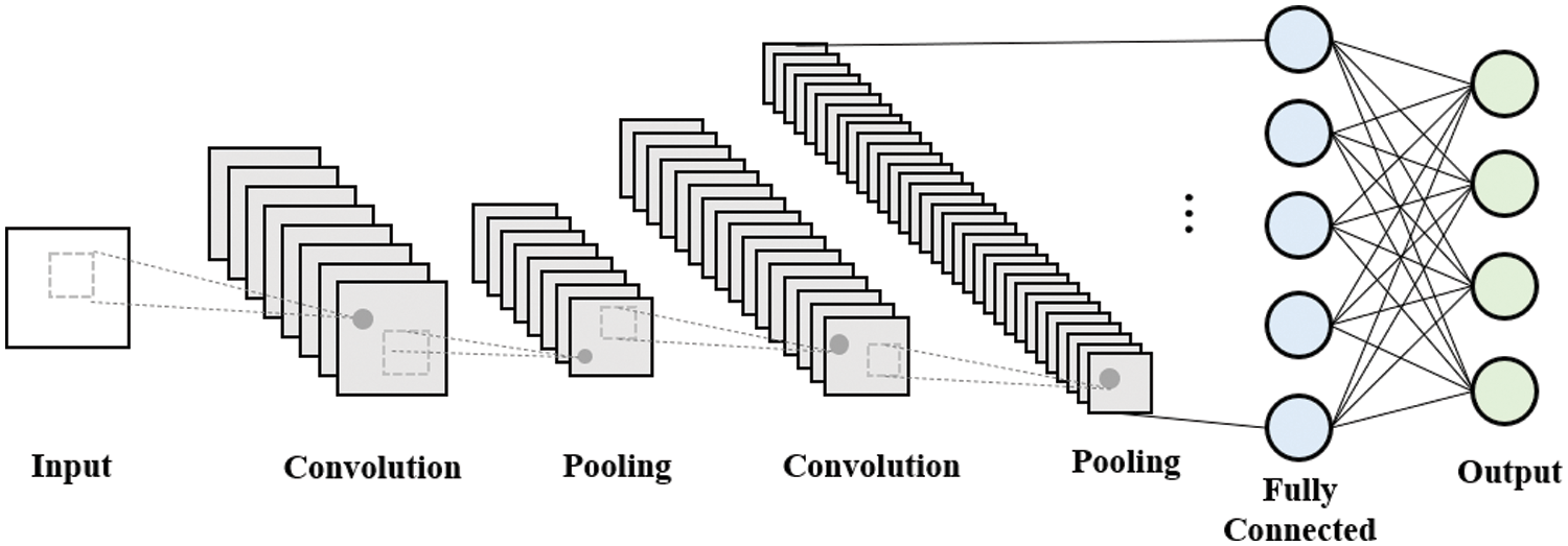
Figure 1: CNN architecture
The convolution layer uses filters (two-dimensional matrices in the form of N × M) to extract features of the image. In two-dimensional data consisting of height and width, N × M-sized filters are traversed at a specified interval, multiplying the overlapping data by the values of the elements in the kernel, and then adding all the multiplied values. The traveling interval is called the “stride”, and if the “stride” is specified as 1, it moves one column at a time and make a convolution. The output from the convolution is called feature map, and the application of the active function to feature map is called activation map. After the convolution process, the output data is smaller than the input data, which goes through a process called padding to prevent the output data from decreasing. Padding is the process of filling the edge of the input data with a specific value by a specified size, usually zeroed.
Pooling layers include max pooling, min pooling, and average pooling. Likewise, the concept of filter and stride is applied to the pooling operation, and usually the filter and stride are identical so that all elements can be processed once. For max pooling, we extract the maximum value from the region where the filter and the data overlap, and similarly, average pooling is the method of extracting the mean. The convolution and pooling operations look similar in that the filter and stride concepts are used, but the pooling operations differ in that no weights exist.
We apply CNN layer to CLARINet to reduce the loss to the original data and make sure that we do not lose the association of each radio signal.
LSTM is used to alleviate the long-term dependence problem of RNN mentioned in Section 1, and the overall structure consists of cells and three gates, such as Fig. 2. Cells have values for arbitrary time intervals, and three gates are responsible for removing unnecessary information or leaving only necessary information that is considered important.
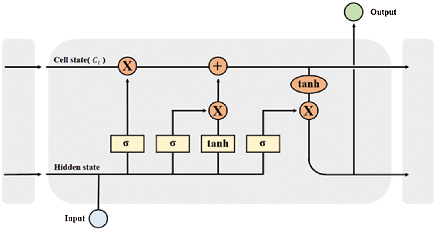
Figure 2: LSTM architecture
Cell state of LSTM is the horizontal line at the top of Fig. 2. Cell state (
The operating process of LSTM, such as Fig. 3, first enters the wireless signal via the forget gate into the input information. Forget gate is a gate that determines what information is reflected in the current information through the operation of Eq. (1) and is determined via sigmoid function.
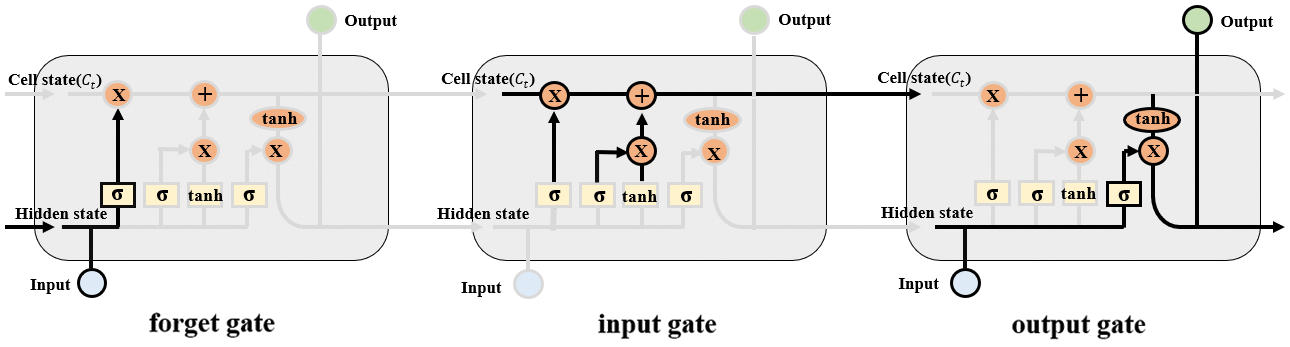
Figure 3: LSTM gate architecture
t represents the time point,
The
The input gate is configured as Fig. 3 and is responsible for remembering the information to store for new information. To remember new information, perform the operations in Eqs. (2) and (3). t represents the time point, and
The
Then, to update the contents of the forget gate and input gate, we go through Fig. 3. Update the information by applying Eq. (4) to
Finally, output gate is the final step in determining which data to output, corresponding to the final step in Fig. 3. The input is entered into the sigmoid function and the value [0, 1] is output, which determines whether to export part of the cell state to output. This output is then passed through the hyperbolic tangent function to the input of the next state.
We leverage CLARINet to automatically do well filtering on given data via CNN layer. Furthermore, we put CNN layers at the forefront of CLARINet to learn important characteristics for each radio signal when classifying radio signals, and to preserve the association of the data, leveraging them to remember the features of radio signals.
Attention references and applies the entire input sentence at each point in predicting the output data, and concentrates the data associated with the data to be predicted and forwards it to the decoder. This mechanism allows us to deliver more data than was previously delivered. The method in which attention mechanism is used is the same as Fig. 4.
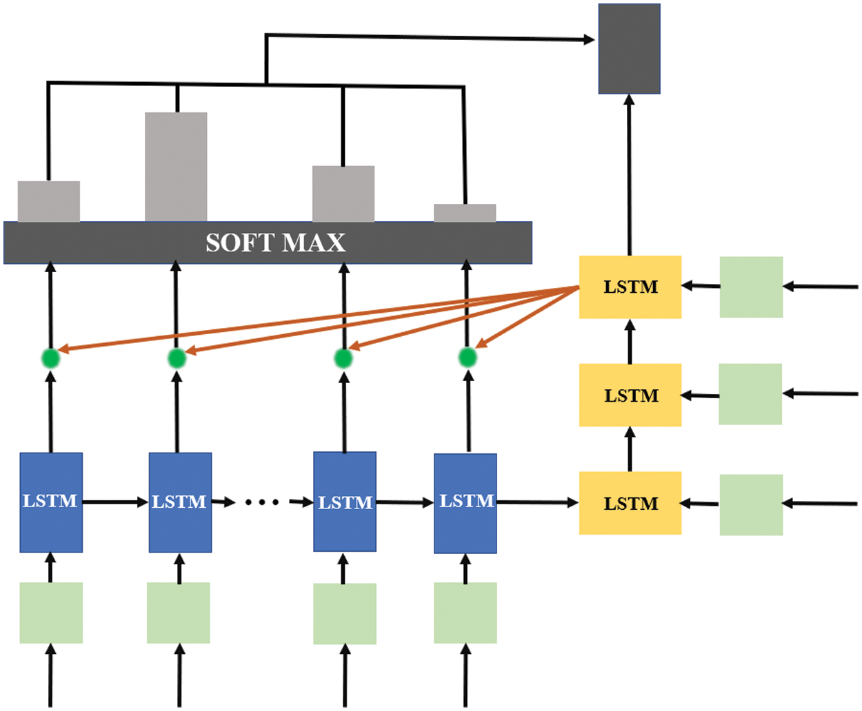
Figure 4: Attention mechanism architecture
The attention score must be obtained to apply the attention mechanism to the layer consisting of LSTM. Attention score is a score that determines the similarity between the hidden state of the encoder and the hidden state st of the encoder at the present time. The softmax function is applied to obtain an attention distribution in which the sum of all values is equal to 1, and each value is an attention weight. This value and the hidden state provide an attention value,
Finally,
We apply an attention mechanism to CLARINet to design an accurate classification by weighting the factors that have a significant impact when distinguishing the features of each radio signal.
Finally, our designed network of CLARINet is designed to reduce conversion, distortion, and loss to the original data through two Conv1D layers, extract the data, and delete the rest of the data except the critical data through two LSTM layers. We then design an attention mechanism to weight important data so that it can be classified focusing on important data when analyzing radio signals. The structure of CLARINet performing this process is the same as Fig. 5.
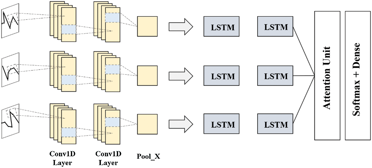
Figure 5: CLARINet model architecture
CLARINet receives the original radio signal for the frequency band signal as input data. We set the number of filters, the underlying property of CLARINet, to 64. Filter determines the filter size, determines the stride, and recognizes the data according to the length of the stride, and generates the activation map as an output. Therefore, CLARINet is designed to generate 64 activation maps over 64 filters.
We designed that data passed through CNN layers remember the features each wireless signal has in order to classify wireless signal over LSTM layer, considering then as important information. It is also designed to remove hidden unit with a 60% chance by leaving the dropout of CLARINet at 0.6. In the LSTM layer, dropout is a type of regularization that solves overfitting and makes it not dependent on any single data through dropout. Through this, the CLARINet model is designed to be overfitted and non-dependent.
Output data through CNN layer and LSTM layer are applied to attention mechanism to solve the gradient loss problem, increasing accuracy, and classified radio signals have an organic relationship with each other. Eventually, data passed to attention mechanisms are classified into 11 radio signals (8PSK, AM-DSB, AM-SSB, BPSK, CPFSK, GFSK, PAM4, QAM16, QAM64, QPSK, WBFM) via softmax regression.
To compare the performance of CLARINet on accuracy, we conducted experiments by selecting a model that combines two CNN layers and two LSTM layers, two CNN layers, one LSTM layer, two LSTM layers, two CNN layers and attention mechanism, as a comparison group. The results of our comparison of the accuracy according to SNR are as shown in Fig. 6.
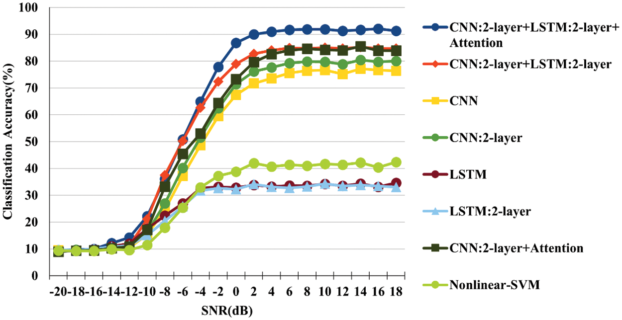
Figure 6: Classification accuracy comparison of CLARINet
If SNR is in the range of −20 to −10 dB, CLARINet and all the seven comparator models selected show less than 10% accuracy, with a narrow rise. Therefore, we analyze the range of SNR based on −10 dB or more to clearly classify the accuracy for CLARINet. Our design of CLARINet shows an average accuracy of 77.40% for SNRs above −10 dB, highest accuracy from 16 dB to 92.03%, and approximately 7.34% higher than that of seven comparators at 16 dB.
We analyze on seven comparator models selected to classify radio signals, and we find that the classification accuracy of models with CNN layers is higher than that of models without CNN layers, and that the accuracy of models with two CNN layers in the range 0 to 18 dB shows an average accuracy of 80%. Furthermore, we compare models based on CNN layers, showing that the two-applied LSTM layers have approximately 2.98% higher accuracy than the single attention mechanism. This shows that CNN layer-based models exhibit high values in the range of 0 to 18 dB in determining accuracy for radio signal classification, and that additional LSTM layer or attention mechanism can be applied to increase accuracy.
The results of CLARINet experiments on −8, 0, 16 and 18 dB on SNR basis to verify accuracy in classifying radio signals in complex radio signal environments were shown as Figs. 7–10.
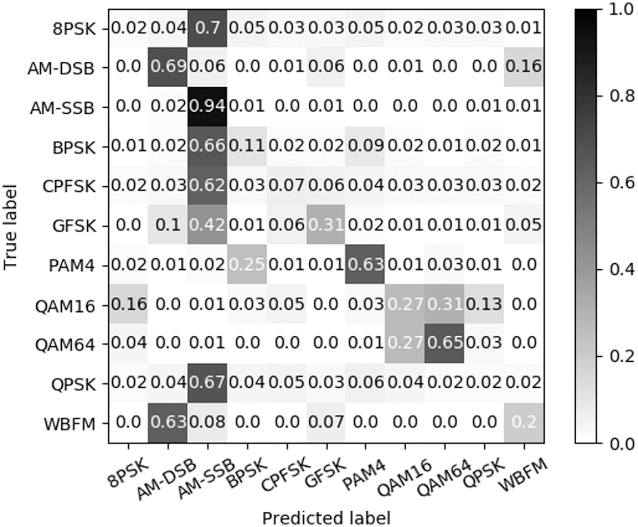
Figure 7: Confusion matrix at SNR −8 dB
SNR below −10 dB has little significance in data results because of its low accuracy, and SNR of −8 dB can be found to be mostly low in accuracy, such as Fig. 7. However, out of a total of 11 modulation techniques, we can confirm that AM-DSB, AM-SSB, PAM4 and QAM64 exceed 50% accuracy, which means that the modulation techniques can be classified to some extent even if noise is severe.
According to Fig. 8, CLARINet shows nearly 90% accuracy on average at SNR 0 dB, and from 4 dB, it can be seen that the accuracy is over 90% on average. In particular, we show that AM-SSB is more classified with an accuracy of over 90%. While the SNR of 0 dB is mostly over 90% accuracy, 8PSK, QAM16, QAM64, and WBFM of the 11 modulation techniques do not exceed 90% accuracy. QAM16 is a subset of QAM64, which often misjudges QAM16 as QAM64 because only the bits that can be sent from one signal are different. WBFM has the lowest accuracy among the 11 modulation techniques, and the signal from WBFM is misclassified as AM-DSB due to the absence of a signal because it was modulated in a real audio stream. At 18 dB SNR, most modulation techniques, such as Fig. 9, show an average accuracy of over 90%, and the accuracy for QAM16 is about 10% higher than the accuracy classified in 0 dB. Furthermore, WBFM was also shown to be 10% higher than the accuracy classified at 0 dB, but relatively lower than other signals.
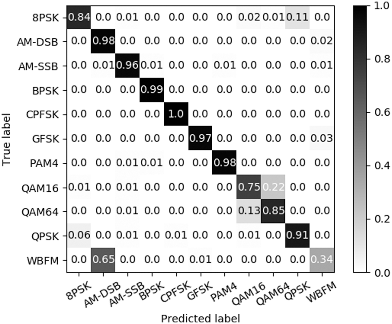
Figure 8: Confusion matrix at SNR 0 dB
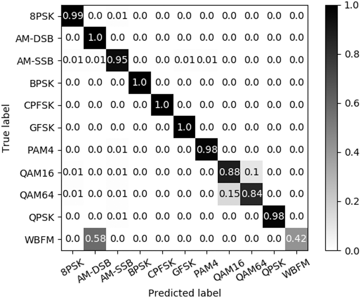
Figure 9: Confusion matrix at SNR 18 dB
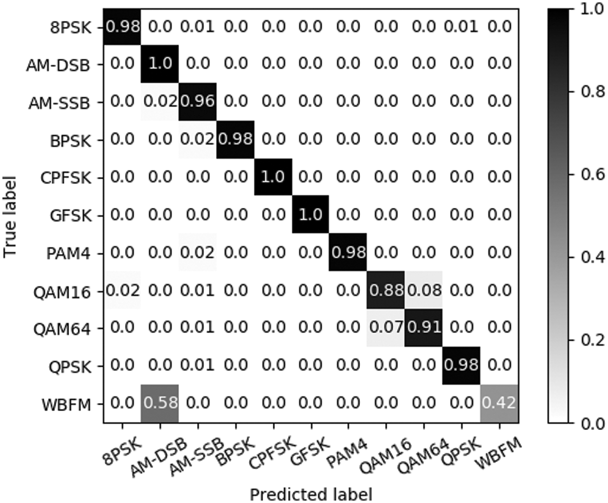
Figure 10: Confusion matrix at SNR 16 dB
We retained the basic properties of CLARINet to verify the experimental results according to the properties of CLARINet, and proceeded with the experiment by changing the number of filters. CLARINet has 64 filters, and the number of filters in the comparison model we selected for comparison is 32, 64, 128, and 256. The experimental results comparing accuracy according to the number of filters are as shown in Fig. 11.
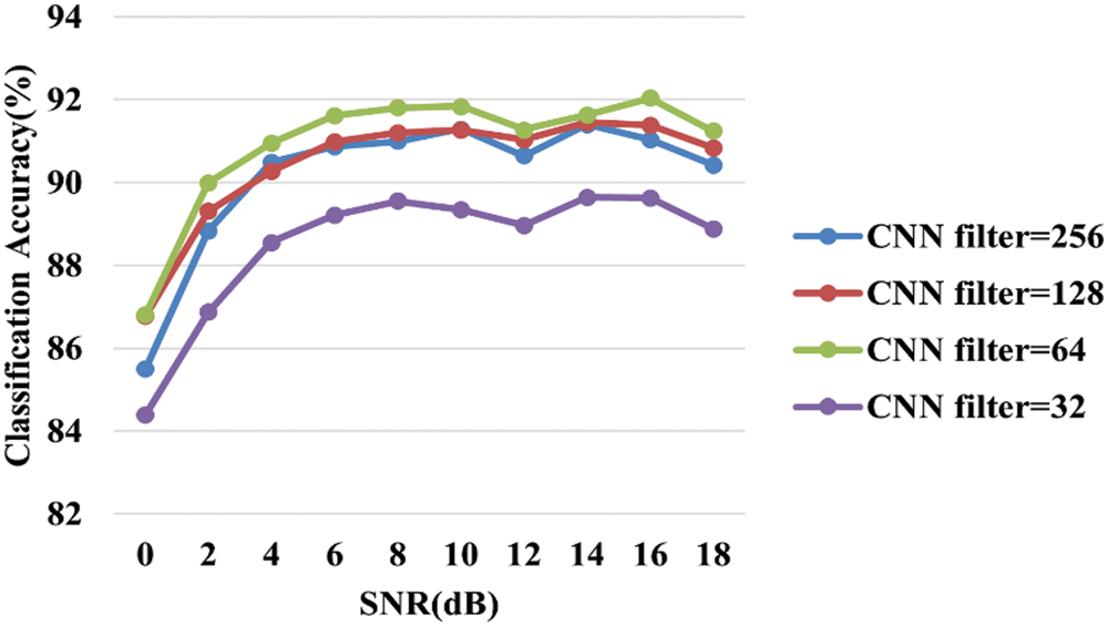
Figure 11: Classification accuracy results by number of filters
When the number of filters is 64, they represent the highest accuracy at all 0 to 18 dB, and the highest accuracy at 16 dB to 92%. While 128 filters and 256 filters represent similar accuracy overall, it can be seen that 128 filters represent slightly higher accuracy. The number of filters increases mainly as the layers are placed behind, with CNN layers located in front of the CLARINet model, with a relatively small number of 64 filters having higher accuracy than 128 filters and 256 filters.
We further analyzed for models with 64 filter and 128 filter indicating high accuracy in Fig. 11. The results of analyzing the two models based on total steps, initial loss, final loss, and runtime are the same as Tab. 1.
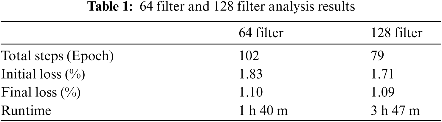
Comparing epochs according to the number of filters, 64 filter shows that Total Steps was 20 more times than 128 filter, which led to more learning. We used categorical_crossentropy as a loss function of CLARINet, and after checking the loss cost, we found that both 64 filter and 128 filter show approximately 1–2% loss. We can see that the final runtime of our designed CLARINet takes about two hours less than 128 filters, depending on the number of filters.
In addition, experimental results comparing accuracy by changing the value of dropout, a regulatory technique to prevent overfitting, were shown as Fig. 12. P, the hyperparameter of dropout, means probability. The probability of dropout temporarily changes depending on the value of this p. Our designed CLARINet is designed by selecting the p value of dropout as 0.6.
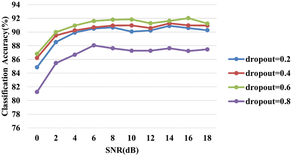
Figure 12: Classification accuracy results by dropout
According to Fig. 12, when dropout is 0.6, it is shown that the highest accuracy is from 0 to 18 dB, and when dropout is 0.4 it is the next highest accuracy. If dropout is 0.8 then low performance indicates that strong regulation indicates low accuracy, and the most common accuracy when left at 20% to 60%. It showed an accuracy of 92% at 16 dB. Through this, we confirm that designing to dropout with a 60% chance at each training step can yield the best performance to improve the accuracy of CLARINet.
Based on the experimental results, we design CLARINet as a structure of two CNN layers, two LSTM layers, and an attention mechanism, with 64 filters on the CNN layer and 0.6 dropout on the LSTM layer, selecting the model with the highest accuracy.
We propose a novel model CLARINet that integrates CNN layer with LSTM layer and attention mechanism as a deep learning-based solution for classifying wireless signals in the IoT environment. Many previous studies have attempted radio signal classification based on original signals with less distortion or loss of radio signals, and have proposed efforts to improve performance on radio signal classification by incorporating various techniques. However, the exact classification of each radio signal has yet to be completely resolved, as radio signals are not separated and propagated, but are complexly propagated in crowded spaces. Previous studies have mainly improved accuracy problems by implementing LSTM-based models. Therefore, we design a model CLARINet with LSTM layer and attention mechanism applied to CNN-based models to accurately classify complex radio signals for each feature.
We show that CLARINet, which is designed to allow wireless signals to obtain individual radio signals in congested spaces, shows approximately 60% accuracy for environments with SNR of −20 to 18 dB, with approximately 92.03% accuracy at 16 dB. Analysis of CNN layer and LSTM layer used in CLARINet structure shows that CNN-based models have an average accuracy of about 40% higher than LSTM-based models. Through this, we have shown that classifying complex radio signals through CNN-based models exhibits higher accuracy than those that do not. Furthermore, we use attention mechanism to weight features on radio signals, remember only important features of radio signals and classify them, identify the possibility of minimizing distortion and loss, and finally confirm that they can be classified into 11 radio signals via softmax regression.
In the future, we plan to improve accuracy by changing the attributes of CLARINet models or by adding layers, and explore ways to improve on misclassifying QAM16 as QAM64 and misclassifying WBFM as AM-DSB. Furthermore, we plan to utilize CLARINet to conduct experiments on image classification to improve the problem by applying it to problems that suffer from data loss or distortion, and simplify our model to optimize the overall performance.
Funding Statement: This work was supported by the National Research Foundation of Korea (NRF) grant funded by the Korea government (MSIT) (No. 2021R1F1A1063319).
Conflicts of Interest: The authors declare that they have no conflicts of interest to report regarding the present study.
1. S. Lim, S. Lee, J. Yoo and C. Kim, “NBP: Light-weight narrow band protection for ZigBee and Wi-Fi coexistence,” EURASIP Journal on Wireless Communications and Networking, vol. 2013, no. 1, pp. 1–13, 2013. [Google Scholar]
2. X. Wu, P. C. Y. Chen and J. Liu, “LSTM network: A deep learning approach for short-term traffic forecast,” Iet Intelligent Transport Systems, vol. 11, no. 2, pp. 68–75, 2017. [Google Scholar]
3. W. Kong, Z. Y. Dong, Y. Jia, D. J. Hill, Y. Xu et al., “Short-term residential load forecasting based on LSTM recurrent neural network,” IEEE Transactions on Smart Grid, vol. 10, no. 1, pp. 841–851, 2019. [Google Scholar]
4. F. A. Gers, J. Schmidhuber and F. Cummins, “Learning to forget: Continual prediction with LSTM,” Neural Computation, vol. 12, no. 10, pp. 2451–2471, 2000. [Google Scholar]
5. F. A. Gers, N. N. Schraudolph and J. Schmidhuber, “Learning precise timing with LSTM recurrent networks,” Journal of Machine Learning Research, vol. 3, no. 1, pp. 115–143, 2002. [Google Scholar]
6. S. Scholl, “Classification of radio signals and HF transmission modes with deep learning,” arXiv:1906.04459, pp. 1–4, 2019. [Google Scholar]
7. S. Tridgell, D. Boland, P. H. W. Leong and P. H. W. Siddhartha, “Real-time automatic modulation classification,” in Int. Conf. on Field-Programmable Technology, ICFPT 2019, Tianjin, China, pp. 299–302, 2019. [Google Scholar]
8. J. Yuan, Z. Z. Yang and Q. P. Liang, “Modulation classification of communication signals,” in IEEE Military Communications Conf., MILCOM 2004, Monterey, CA, USA, pp. 1470–1476, 2004. [Google Scholar]
9. S. Peng, H. Jiang, H. Wang, H. Alwageed and Y. Yao, “Modulation classification using convolutional neural network based deep learning model,” in Wireless and Optical Communication Conf., WOCC 2017, Newark, NJ, USA, pp. 1–5, 2017. [Google Scholar]
10. S. Rajendran, W. Meert, D. Giustiniano, V. Lenders and S. Pollin, “Deep learning models for wireless signal classification with distributed low-cost spectrum sensors,” IEEE Transactions on Cognitive Communications and Networking, vol. 4, no. 3, pp. 433–445, 2018. [Google Scholar]
11. M. Liu, K. Yang, N. Zhao, Y. Chen, H. Song et al., “Intelligent signal classification in industrial distributed wireless sensor networks-based IIoT,” IEEE Transactions on Industrial Informatics, vol. 17, no. 7, pp. 4946–4956, 2021. [Google Scholar]
12. Y. Zhang, J. Wang, G. Wu and Q. Tang, “Wireless signal classification based on high-order cumulants and machine learning,” in Int. Conf. on Computer Technology, Electronics and Communication, ICCTEC 2017, Dalian, China, pp. 559–564, 2017. [Google Scholar]
13. X., Shang, H. Hu, X. Li, T. Xu and T. Zhou, “Dive into deep learning based automatic modulation classification: A disentangled approach,” IEEE Access, vol. 8, pp. 113171–113284, 2020. [Google Scholar]
14. L. Huang, W. Pan, Y. Zhang, L. Qian, N. Gao et al., “Data augmentation for deep learning-based radio modulation classification,” IEEE Access, vol. 8, pp. 1498–1506, 2019. [Google Scholar]
15. M. Sadeghi and E. G. Larsson, “Adversarial attacks on deep-learning based radio signal classification,” IEEE Wireless Communications Letters, vol. 8, no. 1, pp. 213–216, 2018. [Google Scholar]
16. L. Huang, Y. Zhang, W. Pan, J. Chen, L. P. Qian et al., “Visualizing deep learning-based radio modulation classifier,” IEEE Transactions on Cognitive Communications and Networking, vol. 7, no. 1, pp. 47–58, 2020. [Google Scholar]
17. T. J. O'Shea, N. West, M. Vondal and T. C. C. Bradley, “Semi-supervised radio signal identification,” in Int. Conf. on Advanced Communication Technology, ICACT 2017, PyeongChang, Korea, pp. 33–38, 2017. [Google Scholar]
 | This work is licensed under a Creative Commons Attribution 4.0 International License, which permits unrestricted use, distribution, and reproduction in any medium, provided the original work is properly cited. |