Efficient Computer Aided Diagnosis System for Hepatic Tumors Using Computed Tomography Scans

Yasmeen Al-Saeed; Wael Gab-Allah; Hassan Soliman; Maysoon Abulkhair; Wafaa Shalash; Mohammed Elmogy

doi:10.32604/cmc.2022.023638

Yasmeen Al-Saeed1,2, Wael A. Gab-Allah1, Hassan Soliman1, Maysoon F. Abulkhair3, Wafaa M. Shalash4 and Mohammed Elmogy1,*

1Faculty of Computers and Information, Mansoura University, Mansoura, 35516, Egypt
2Faculty of Computers & Artificial Intelligence, South Valley University, Hurghada, 84511, Egypt
3Faculty of Computing and Information Technology, King Abdulaziz University, Jeddah, 21589, Saudi Arabia
4Faculty of Computers and Artificial Intelligence, Benha University, Banha, 13511, Egypt
*Corresponding Author: Mohammed Elmogy. Email: melmogy@mans.edu.eg
Received: 15 September 2021; Accepted: 05 November 2021

Abstract: One of the leading causes of mortality worldwide is liver cancer. The earlier the detection of hepatic tumors, the lower the mortality rate. This paper introduces a computer-aided diagnosis system to extract hepatic tumors from computed tomography scans and classify them into malignant or benign tumors. Segmenting hepatic tumors from computed tomography scans is considered a challenging task due to the fuzziness in the liver pixel range, intensity values overlap between the liver and neighboring organs, high noise from computed tomography scanner, and large variance in tumors shapes. The proposed method consists of three main stages; liver segmentation using Fast Generalized Fuzzy C-Means, tumor segmentation using dynamic thresholding, and the tumor's classification into malignant/benign using support vector machines classifier. The performance of the proposed system was evaluated using three liver benchmark datasets, which are MICCAI-Sliver07, LiTS17, and 3Dircadb. The proposed computer adided diagnosis system achieved an average accuracy of 96.75%, sensetivity of 96.38%, specificity of 95.20% and Dice similarity coefficient of 95.13%.

Keywords: Liver tumor; hepatic tumors diagnosis; CT scans analysis; liver segmentation; tumor segmentation; features extraction; tumors classification; FGFCM; CAD system

The liver is one of the most vital organs in the human body. It is responsible for at least 500 essential functions for the body, such as regulating blood clotting, filtering blood from waste substances and medications, and raising immune factors to fight infections. Hence, early detection and diagnosis of liver problems are critical tasks. The morbidity of liver cancer has increased three times when compared to 1980 [1]. Over the last decade, the percentage increased by about 3%. Men are significantly more likely to be more morbid to liver cancer by three times than women. Liver or hepatic cancer is expected to be responsible for about 31,780 deaths per year (21,600 men and 10,180 women). Hepatic cancer was ranked the 5th most common death causes in men and the 7th in women [2]. Early detection, diagnosis, and accurate staging of liver tumors are essential issues in radiography.

Chronic liver disease (CLD) development is identified through many phases; each has physiological and pathological features. The early phase of liver cancer starts when fats are increased in hepatocytes. This phase is called fatty liver infiltration or steatosis [3]. In the liver damage phase, fibrosis appears. The evolution of fibrosis relies on the source of hepatic failures, such as chronic hepatitis. The late phase of CLD is cirrhosis, and it refers to a deficiency of liver functionality due to long-term damage. Cirrhosis is classified into two categories, namely decompensated and compensated cirrhosis. When cirrhosis reaches late phases, the patient is diagnosed with primary liver cancer [4,5].

The staging and detection of CLD are achieved using medical imaging modalities with computer-aided diagnosis (CAD) systems [6]. For liver cancer diagnosis, computed tomography (CT) imaging modality is used. CAD systems are computer methods that extract hidden knowledge from acquired medical images to enhance disease diagnosis accuracy. The hepatic CAD systems are mainly concerned with developing methodologies and techniques to enhance medical images’ quality, improve the diagnosis accuracy, and detect or segment liver tumors [7]. Liver tumors CAD systems have common implantation stages; the liver segmentation, tumors segmentation and tumors classification or diagnosis.

Manual liver and tumor segmentation from CT scans is tedious and prohibitively time-consuming for a clinical setting. The primary automatic liver segmentation challenges can be summarized as follows. First, the liver has high intensities values overlap with its surrounding organs, especially the heart, right kidney, and spleen. This overlap makes it more challenging, especially for the automatic liver segmentation process. Second, the liver has various shapes across subjects. Finally, the presence of tumors or other abnormalities may result in severe intensity inhomogeneity [8]. The task of automatically segmenting liver tumors is considered immensely challenging due to various factors. The liver stretches over 150 slices in each CT scan file, with indefinite tumor patterns, low-intensity contrast between tumors and the rest of the liver tissues, variance in liver shape and size through CT slices in a single subject as well as between different subjects, and intensity intersection between liver and other abdomen organs [9,10].

Tumor classification systems aim to classify hepatic tissues into either normal, malignant, or benign. Classification accuracy mainly depends on the quality of the extracted features. Features extracted from medical images refer to quantitative measurements beneficial in the structure or tissue pathology classification process. Features can be extracted in both spectral or the spatial domain. A subset of the most robust features is selected for enhancing classification quality and reducing processing complexity. Feature selection methods use search strategies, categorized as exhaustive, heuristic, and non-deterministic approaches [11]. Extracted hepatic features can be either textural or statistical features. Texture-based features measure appearance and textural changes between healthy/unhealthy hepatic tissues. Textural features include Gabor energy, homogeneity, energy, contrast, and correlation. Statistical features may include uniformity, entropy, and mean grey-level intensity between healthy/tumor tissues [12]. The advanced classification systems aim to classify the liver tumors into more specific categories, such as normal, cyst, hemangioma, and HCC [13].

The proposed CAD system is comprised of several stages. The first stage is CT scans quality enhancement stage. At this stage, the CT image is converted to greyscale, contrast-enhanced with histogram equalization, and filtered with median filtering. At this point, the input CT image becomes uniform, homogeneous, and more suitable for the segmentation process. The second stage is the liver segmentation stage. This stage aims to segment the liver from the rest of abdomen organs using the fast-generalized fuzzy C-means (FGFCM) method. The third stage is tumors segmentation at which the segmented liver is passed to an adaptive thresholding method to segment detected tumors. The final stage is the diagnosis stage at which the segmented tumors are classified into malignant or benign using support vector machines (SVM) classifier.

This paper proposes a CAD system framework for differentiating benign and malignant liver tumors. The proposed system was able to reduce the effect of impulse noise from the CT scanner on the quality of the segmentation process using adaptive median filtering (AMF). It was also able to solve the problem of high intensities overlap between the liver and the rest of abdomen organs by selecting CT slices at which the liver can be differentiated and enhancing contrast using the adaptive histogram equalization (AHE) method. High-quality segmentation of the liver was achieved using FGFCM since it has high ability to preserve correlation between image pixels. The diagnosis of the hepatic tumors was implemented using a combination of statistical intensity-based features such as mean, standard deviation, and skewness and textural-based features such as gray-level difference matrix (GLDM). The performance of the proposed method was evaluated using three bench-marks datasets and different performance metrics were calculated. The main contribution of our proposed CAD system can be outlined in the following points:

• Proposing a comprehensive framework for differentiating benign and malignant liver tumors from various datasets.

• The effect of impulse noise from CT scanner on quality of segmentation process was reduced by using adaptive median filtering (AMF).

• The liver and abdomen organs intensities values overlap were solved by first selecting only CT slices at which liver can be differentiated, and enhancing contrast using adaptive histogram equalization (AHE) method.

• Using FG-FCM for the liver segmentation to solve the problem of noise sensitivity with high details-preserving abilities to provide high quality segmentation.

• The proposed method aims mainly to classify segmented tumors into benign/malignant tumors using a combination of statistical intensity-based features and textural based features. Intensity features include the mean, standard deviation, and skewness. Textural features include GLDM.

• The performance of the proposed method was evaluated using three bench-mark datasets. Different performance metrics were calculated.

The rest of this paper is ordered as follows. Section 2 reviews the related work. Section 3 discusses the proposed CAD system for the liver/hepatic tumor segmentation and diagnosis. Section 4 presents experimental results and further discussion. Section 5 summarizes the most important findings of this work.

Several techniques had been proposed to efficiently solve the problem of the liver and tumors segmentation from abdominal CT scans. Those techniques can be classified into two categories. The first category is the direct approach that focuses solely on tumor segmentation by segmenting tumors alone without segmenting the liver as an intermediate stage. The second category is the indirect approach that first segments the liver and then segments the tumor.

Moltz et al. [14] proposed a hybrid method to segment liver tumors. This method first segmented the liver by using a rough segmentation based on the adaptive thresholding approach. Then, tumors were segmented using model-based morphological processing. The main drawback of this method was that it required the user to specify the center of the region of interest (ROI) for tumor segmntation algorithm. Huang et al. [15] proposed an automated liver segmentation hybrid method. First, the liver intensity range was determined in regards to the input liver volume data. The ROI was then identified using an atlas-based affine and non-rigid registration. To achieve high-quality segmentation, primary -liver tumors were segmented based on grey level and distance prior knowledge in the final stage. The results demonstrated that this method had the capability to be used as a clinical tool. However, this method had high computational complexity. Wong et al. [16] proposed a semi-automatic method based on region growing segmentation. They used CT scans as the primary imaging modality. To guarantee that region's shape and size were grown within acceptable limits, knowledge-based constraints were used. This method required ROI to be identified manually by selecting two CT images points before the region grew. Pohle et al. [17] proposed an adaptive region growing technique. This method had the advantage of automatically learning about the homogeneity criterion from the characteristics of segmented regions. However, if the segmented region is heterogeneous, this method was inefficient and resulted in under segmentation.

Li et al. [18] proposed a hybrid method for liver tumor segmentation. This method integrated two segmentation approaches, which are fuzzy C-means (FCM) and level set segmentation. They first used FCM for segmentation. Then, they implemented the level set for fine delineation. The output of those two steps was integrated using some morphological operations. This method had a high processing time due to the use of the level set approach. Zhou et al. [19] provided a performance benchmark study for three semi-automatic liver tumors- segmentation methods. These three methods involved region growing with knowledge-based rules, propagational learning for tumor pixels classification, and region growing based on the Bayesian rules. The results showed the superiority of the first two methods over the third. Abdel-Massieh et al. [20] proposed an enhanced threshold-based method for segmenting liver tumors from CT scans. They started by improving the grey level intensity contrast of the input image. The main drawback of this method was its severe sensitivity to noise.

Kumar et al. [21] proposed an automatic and effective liver tumors segmentation method from CT images. The method used confidence connected region growing technique to segment liver and alternative FCM clustering to segment tumors. This method was validated using 10 cases of CT scans. Zhao et al. [22] proposed a hybrid liver segmentation method based on FCM and multilayer perceptron. They used a dataset of ten subjects with 40 slices per subject. The quality of CT scans was enhanced using a threshold method. The initial liver edges were marked using FCM clustering and morphological reconstruction filter. Then, the segmented liver results were used to train a multilayer perceptron neural network. The process was stopped when the network was able to segment the liver through all slices successfully.

Danciu et al. [23] proposed the usage of tumor volume, diameter, and size as the main texture features. This paper selected tumors features based on the concept of minimum redundancy/maximum relevance. This helped in the selection of unique textural features with lower redundancy as possible. Also, the dependency of extracted features was maximized.

Ji et al. [24] proposed the usage of structure and context properties to segment tumors from surrounding liver tissues in 3D CT scans. This method had the advantage of automatically acquiring implicit tumors shape characteristics using the active contour model (ACM) method. Besides, it showed good segmentation performance due to its ability to combine multiple atlas scans that enhanced segmentation accuracy. Finally, it improved the classification performance by using enhanced mean shift method and reduced segmentation time. However, this method required ground truth (GT) to be specified manually by the user. Smeets et al. [25] proposed a tumor segmentation method based on the level set technique. The algorithm started with a seed point placed inside the tumor to apply a spiral scanning technique. The level set evolves according to a seed image obtained by statistical pixel classification with supervised training. This method was highly user-dependable since it required the user to specify the seed point at the center of the tumor and clarify a maximal radius by placing a point in the surrounding liver tissue.

Moghe et al. [26] proposed an automatic liver tumor segmentation method from CT images. This method was based on the threshold segmentation approach. They used statistical moments and texture measures to select threshold values. However, the process of selecting threshold values is still a very challenging task. Yussof et al. [27] proposed a liver/tumor segmentation method. First, the liver was segmented using morphological method. Then, the tumor was segmented using anisotropic diffusion, adaptive threshold and connected component algorithm. The results showed liver's over-segmentation near the muscles and liver's under-segmentation when lesions were near the liver boundaries. Hame [28] proposed a method for liver and tumor segmentation. This method first used morphological features and thresholding techniques to segment the liver from the rest of the abdomen organs. Segmentation quality was enhanced using a fuzzy clustering approach. Liver tumors were segmented by fitting a geometric deformable model based on the membership function generated by the clustering method. This method achieved high accuracy when rough segmentation process was successful. However, rough segmentation had a low robustness which affected the overall performance of this method.

Adcock et al. [29] proposed a method to classify different liver tumors: cysts, metastases, hemangiomas, hepatocellular carcinomas, focal nodules, abscesses, and neuroendocrine neoplasms. Their proposed CAD system integrated 2D persistent homology, bottleneck matching and SVM. The output of this method had the advantage of being suitable to be passed to machine learning algorithms. However, this method suffered from difficulties presented when large tumor pixels were normalized. It led to misclassifications. Huang et al. [30] proposed a technique to categorize tumors into either benign or malignant. The tumor region was segmented using the FCM clustering method. Features were extracted using Fast Discrete Curvelet Transform (FDCT) from the segmented tumors. Feed Forward classification method was then used to label tumors as benign or malignant tumors. This method had the advantage of not requiring any user interaction to correct any poor segmentation.

Li et al. [31] proposed a hybrid method to solve the haptic tumors’ classification issue. This method started with some prior knowledge as radiologists identified tumor regions on the CT scan images. This prior knowledge reduced the time consumed during the segmentation process and eased the feature extraction process. Extracted features included spatial grey scale metrics such as dependency, run length, and different metrics. Multiclass Support Vector Machine (MSVM) was then implemented to label haptic tissues into either primary hepatic carcinoma, hemangioma, or normal tissues. MSVM used one-against-all (OAA) and one-against-one (OAO) techniques to decompose the three-class classification problem into a series of binary classifications.

Automatic liver segmentation is still an open problem. It often fails when the liver is in a complex shape, and it typically time consuming in the training stage. In the case of semi-automatic liver segmentation, user interaction could complement computer capabilities to recognize the liver region and its boundaries through CT scans. This made semi-automatic superior when it comes to accurate liver segmentation. The main limitation of semi-automatic liver segmentation methods is the dependency between the quality of segmentation output and the operator user skills, which may be affected by the user's errors and biases.

Despite the significant advancements in liver medical image analysis research, there were some significant challenges. The first challenge was the sensitivity to the noise. Segmentation methods with high noise sensitivity might fail to contour the liver and tumors accurately. The second challenge was that the discussed automatic approaches might consume long computational time in the training stage to learn different liver shapes through CT slices. This may result in high implementation complexity.

The proposed method was able to solve the main challenges of the liver medical image analysis. First, it used the AMF method to reduce segmentation sensitivity to impulse noise imposed by the CT scanner. It also used the FGFCM segmentation method, which had high noise robustness with high detail-preserving ability. Second, it solved automatic liver segmentation challenges resulting from different liver structures through CT slices. This was achieved by selecting only CT slices at which the liver was differentiable and discarded the rest. Finally, the proposed method solved the liver and its neighboring organs’ problem with the same range of intensities values. These organs made segmenting the liver automatically a complex and challenging task since they might have the same pixel intensity values as the liver. The proposed method solved this problem by enhancing liver-to-abdomen contrast using the AHE method, making the liver region easier to segmented.

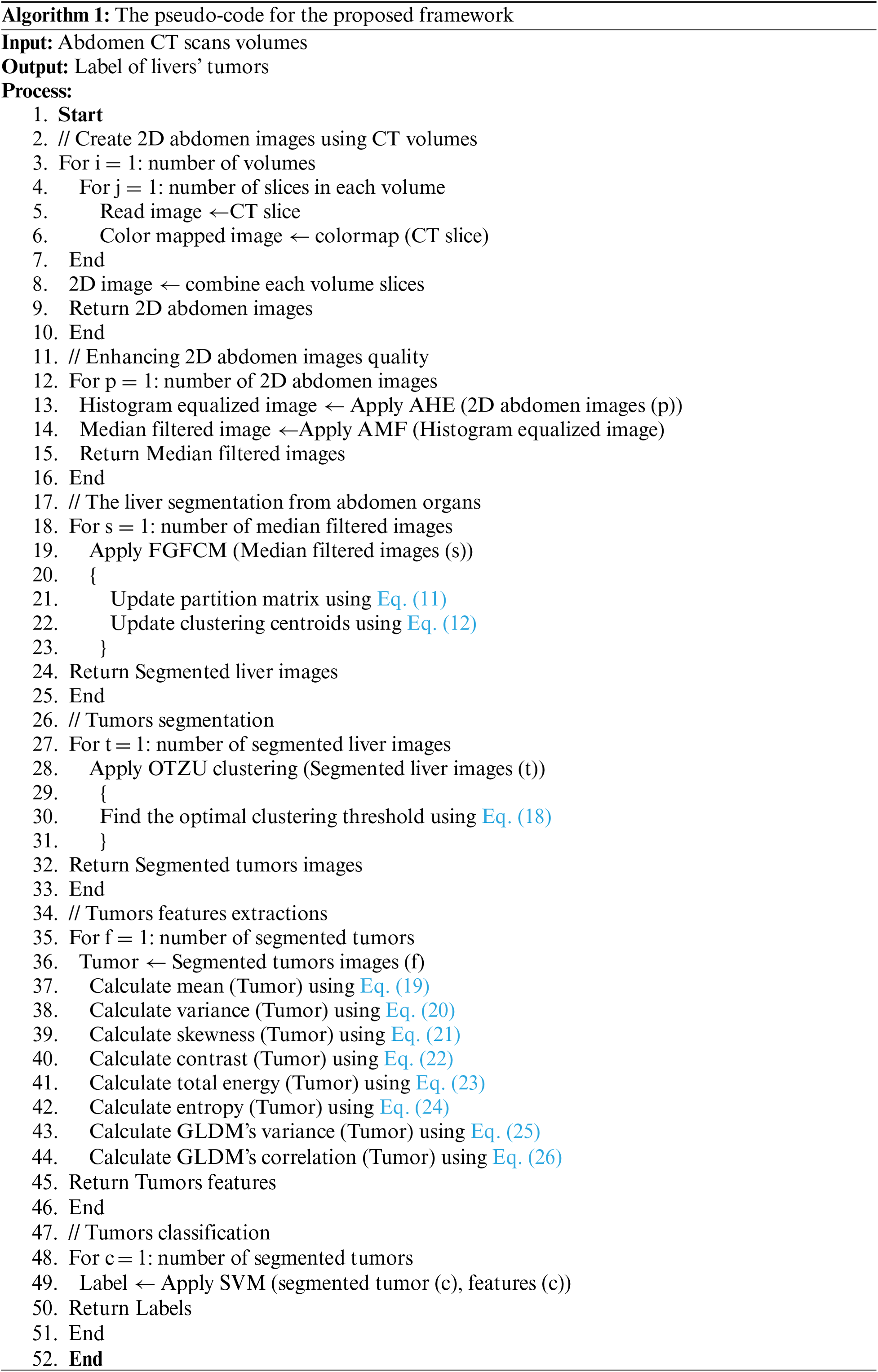
The proposed CAD system aims to assist radiologist decisions by accurately classify hepatic tumors into either malignant or benign tumors. It uses statistical and textural features from extracted tumors to utilize the classification process. The overall performance of the proposed system was evaluated using three benchmark datasets with different characteristics. Fig. 1 illustrates the basic structure of the proposed system, which has three main stages: liver segmentation, tumor segmentation, and tumor classification. Algorithm 1 list the pseudo-code for the proposed framework.

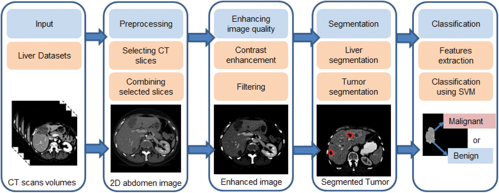
Figure 1: The proposed CAD system for liver tumor segmentation and diagnosis framework

CT scanning is an imaging technique that uses X-ray beams and rotates around the body to generate cross-sectional images (i.e., slices) of the imaged body organ. After acquiring a sufficient number of successive slices, the CT scanner computer creates a 3D representation of the imaged body organs by stacking together the acquired slices. CT scanners, as opposed to X-ray scanners, use detector arrays rather than a single X-ray film. Those arrays are placed in the opposite direction of the beam source. CT imaging is considered the best imaging modality for detecting any potential tumors or abnormalities in soft tissues, such as the brain, heart, liver, and lung. CT scans of internal organs such as the liver have the advantages of providing greater clarity, revealing more details, and minimizing radiation exposure compared to regular X-ray exams. In standard X-rays, a beam of energy is aimed at the body part being studied. A plate behind the body part captures the variations of the energy beam after it passes through the skin, bone, muscle, and other tissue. While much information can be obtained from a standard X-ray, a lot of detail about internal organs and other structures is not available [32].

In this paper, CT scans were acquired from three benchmark datasets; Computer-Assisted Intervention Society (MICCAI) liver segmentation challenge (Sliver ‘07 dataset, 2016) [33], Liver Tumor Segmentation Challenge dataset (LiTS17) provided by IEEE International Symposium on Biomedical Imaging (ISBI-2017) [34] with MICCAI-2017, and 3Dircadb dataset provided by Research Institute against Digestive Cancer [35].

To enhance the accuracy of further processing steps, CT scans were gone under the preprocessing stage. This stage aims to reduce computation complexity and enhance further segmentation processes. In MICCAI-Sliver07 and LiTS17 datasets, computation complexity was reduced by selecting only the most significant slices at which the liver is dominant and discarding the rest of them. After that, the quality of selected images was enhanced by color mapping their intensities to be in the range of [0 255]. For the 3Dircadb dataset, the pixel values range from −1000 to 4000 on the Hounsfield scale [36].

The quality of color-mapped images was enhanced using AHE [37]. AHE achieves a higher contrast version of the input image by spreading out its intensity values and the total range of values within it. This technique is effective when the image is represented by similar intensity values, such as when the background and foreground are both bright at the same time or both are dark at the same time. The histogram of a digital image I with L discrete intensity levels is defined by Eq. (1). AHE enhances I by using the transformation function E which is defined by Eq. (2).

The impulse noise imposed by the CT scanner highly affects the segmentation process, since segmentation methods have high noise sensitivity. The proposed system reduced its effect using AMF method [38]. AMF detects pixels that were affected by impulse noise using spatial processing. AMF uses an adaptive window to label pixels as noisy pixels. It compares each pixel in the input image to its surrounding neighbor pixels in the window. An impulse noise-affected pixel has a different gray-level value than most of its neighbors and is not structurally aligned with the pixels to which it is similar. It replaces noise pixels values with the median value of their similar neighbor pixels and it has the advantage of preserving the edges and detailed information of the image. By the end of this stage, the CT scans are uniform, homogeneous and more suitable for the segmentation process (see Fig. 2).

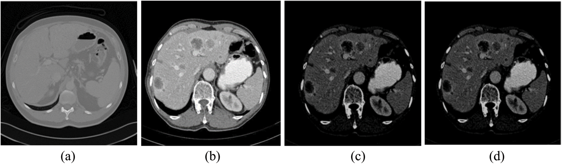
Figure 2: The experimental results of the proposed method for steps 1–4 (a) Original CT scan, (b) Color mapped, (c) Contrast enhanced using AHE and (d) Filtered scan using AMF

The main goal of this step is to segment the liver from the rest of the abdominal organs. FCM [39] is a method by which a single data point can belong to all clusters with various degrees of membership. This method begins by dividing n input metrics into C fuzzy clusters, computing the center of each cluster, and finally maximizing the similarity index value of the objective function. Optimizing the objective function guarantees that all data points at the same cluster have same characteristics. FCM takes fuzzy partitions to make each given input value between 0 and 1 to determine its degree of membership to a class. After normalizing, the combined membership of a dataset is represented as in Eq. (3). Let X be a set of n values of X0, X1…., Xn, and V be a set of c centroids V0, V1……., Vc, the FCM will cluster X points into C cluster by minimizing Eq. (4).

where 1 ≤ m ≤∞ is the fuzzifier, vi is the ith centroid corresponding to cluster βi, uij [0,1] is the fuzzy membership of the pattern xj to cluster βi.

FCM has several main disadvantages. First, it doesn't consider any spatial dependency between pixels in the image and treats each pixel as an individual point. Second, the FCM membership function is based on intensity values similarities between pixels and clusters centers. This means that when segmenting noisy and inhomogeneous CT scans, the sensitivity to noise is increased, resulting in inaccurate segmentation. Last but not least, the original FCM, with its two extensions FCM-S1 and FCM-S2 [40], suffered from being sensitive to noise and outliers when there is no prior- knowledge of the noise. To make a trade-off between noise sensitivity and preserving image details, the new parameter α was added to the equations. The selection of α value was a very complex and time-consuming process. The segmentation process with FCM-S1 and FCM-S2 versions was dependable on image size (i.e., the larger the image, the more time it takes to segment it).

FGFCM [41] was proposed to solve FCM problems and take local spatial information into account during the segmentation process. This was achieved by replacing parameter α with the new parameter Skj. This parameter incorporates two parameters Ss,kj and Sg,kj which indicates local spatial and local grey level relationships, respectively. It is defined by Eq. (5).

where the kth pixel is the center of the local window with a size of n × n, and jth pixels are the neighboring pixels within the window area. The local spatial Ss,kj defined by Eq. (6).

where (pk,qk) represents the spatial coordinates of the kth pixel, λs represents scale spread factor for Ss,kj which indicates its change characteristics, and Ss,kj represents the damping range of the neighboring pixels with spatial distances from the central pixel. The local grey-level Sg,kj is defined by Eq. (7).

where xk represents the central pixel's intensity value within the window, xj represents jth pixel's grey-level value within the same window, λgdenotes the global spread scale factor of Sg,kj.σg,k is a function that represents the local density of the neighboring pixels and is defined by:

where σg,k represents the homogeneity degree of grey-values within the local window. The smaller it gets, the more homogenous the local window is. σg,k reflects the damping in grey-level values by automatically changing with respect to different grey-levels values of all image pixels. FGFCM objective function incorporates both spatial and grey-level values is represented by Eq. (9).

where vi indicates the fuzzy membership of pixel k with respect to class i, γk is the count of the pixel with the same grey-level value as pixel k, where k is 1, 2,……, q. The q value represents the count of all grey-level in the input image and is much smaller than N. The output image is generated by Eq. (10).

where xj represents grey-level values neighboring pixels with respect to the window's central pixel xk. Nk represents a set of all pixels in the range of local window, skj is the similarity score of two-pixel k and j. skj can be used to represent jth weight, and ξk is the weight of kth pixel in the weighted summed output image. The clustering/partition matrix and clusters centroids, respectively. They are iteratively updated using Eqs. (11) and (12).

By incorporating both spatial and grey-level similarity into its objective and membership functions, FGFCM has high noise sensitivity robustness and detail-preserving abilities. It also eliminates the need for the adjustment factor α. Since FGFCM depends on the number of image grey-levels q rather than its size N, it achieves fast segmentation with low time complexity.

Segmentation methods based on the thresholding approach are considered one of the simplest and fastest segmentation methods. Those methods work by the assumption that images are composed of different regions and each region has different pixels intensities. The optimal threshold value is usually selected visually, leading to poor segmentation results (i.e., over or under segmentation results). To solve the problem of optimal threshold selection, some methods were proposed, such as the OTZU method to automate selecting the optimal threshold value [42].

The proposed CAD system uses OTZU thresholding to segment hepatic tumors. OTZU method aims to compute the optimal value global threshold for the whole input image. OTZU method starts by presuming that the input image has two-pixel classes or a bimodal histogram. Then, it computes the optimal threshold that minimizes the intra-class variance (the variance within the class) for the two pixels classes. The intra-class variance could be defined using a weighted equation of each class's variance, as Eq. (13) presents.

where the weights qi can be calculated by Eqs. (14) and (15), and they represent the probability for each class i. Finally, the variances of the two-class are given by Eqs. (16) and (17).

The process can be terminated at this point. The algorithm can continue by calculating inter-class variances for all thresholds t, and selecting t value minimizes variances. OTZU exploits the correspondence between the inter-class and intra-class variances given by Eq. (18) to reduce calculations complexity. Minimizing the intra-class variance is equivalent to maximizing the inter-class variance. The threshold value that maximizes the inter-class variance is the optimal threshold value.

where σbrepresents the inter-class variance and σw represents the intra-class variance.

After completing tumors detection and before tumors classification, the features extraction step must be implemented. Features extraction methods fall into three categories: intensity, textural, or shape features [43]. Tumor intensity features indicates the statistical correlation of pixel's grey-level values within the tumor area such as histogram, mean, variance, skewness, entropy, kurtosis, and tumor area energy. Textural features indicates homogeneity, contrast, energy, and the correlation between tumor pixels such as Gabor-Energy, GLDM. Shape features include tumor area, smoothness, solidity, compactness, and sphericity for the tumor. Generally, features from different categories are combined for sophisticated hepatic tumor classification. For instance, if the tumor is not growing and tending to have sharp boundaries and a homogeneous structure with low-intensity colors, it is classified as a cyst. If the tumor is growing peripherally or nodular, then it could be a hemangioma. Hemangioma is considered the most common liver tumor. If the tumor is not a hemangioma or cyst, it is classified into either hyper-vascular or hypo-vascular tumors [44].

The proposed CAD system classify the segmented tumors into either benign or malignant tumors using a combination of statistical and textural-based features. The used intensity features include the mean, standard deviation, and skewness while the used textural feature is GLDM. For each image tumor, the mean (μ) represents the average of all tumor pixels intensities and is calculated by Eq. (19).

where L(a,b)is pixel (a, b) intensity value within the tumor area. M is the total number of tumor pixels. Standard deviation (σ) refers to intensity dispersion and is calculated by Eq. (20).

where h is the histogram values for tumor intensities. The histogram represents the number of all grey-level values within the tumor area. As the CT scan is a color-mapped 8-bit grey-level image, the number of its grey-level ranges from 0 to 255. The histogram is calculated by first initializing the histogram values to zero. Then, counting the number of pixels with the same intensity value as a particular value. The counts are then returned as the 2D histogram (a vector of the count values). Histogram symmetry degree is referred to as skewness and calculated by Eq. (21).

GLDM [45] is a textural feature extraction method that depends on the occurrence of two pixels with different absolute grey-level intensities, with displacement value δ. GLDM calculates the probability density functions (PDF) for the tumor area. For any displacement vector δ within tumor area, the estimated PDF D(i,δ) is calculated by Eq. (22).

where sδ(x,y)=|s(x,y)−s(x+Δx,y+Δy)|. Five textural features are calculated from D(i,δ), which are contrast, entropy, mean, homogeneity, and correlation. The contrast is calculated by Eq. (23).

where p (x, y) is the GLDM-PDF for pixels x and y. The total energy is also referred to as angular second moment, is defined by Eq. (24). Entropy is calculated by Eq. (25). Variance is used as an indication of image homogeneity and is calculated by Eq. (26).

where μ1, μ2, σ1σ2are the mean and the variance of GLDM, respectively, after the first component and second component. Extracted statistical and textural features are used to input SVM to label detected tumors into either malignant or benign tumors.

In this paper, classification stage aim to predict class labels (i.e., malignant/benign) of unknown data (i.e., segmented tumor) using extracted features. The classification process was implemented based on the radiological charactersitics of different hepatic tumors in [46]. SVM is a binary classifier, and it divides the input points into two classes by constructing an N-dimensional hyper separation plane [47]. The input data points must be transformed from their dimension into a higher dimension since input points may not be linearly separable in their own space. This can be achieved by using Eq. (28).

SVM maintains lower computational complexity by using kernel functions. The most commonly used kernel functions are radial basis function (RBF), linear, sigmoid, and polynomial kernel functions [48]. This paper used the RBF kernel function. RBF kernel of two points f and f~ which denote features vectors in the input space is defined by Eq. (29).

where ∥f−f¯∥2 is the square of the Euclidian distance between feature vectors f and f~. RBF(f,f¯) value is in the range of 0 and 1. It has the value of 0 when two features’ vectors are different (i.e., large distance) and 1 when the two vectors are the same (i.e., f = f~). The RBF feature space has an infinite number of dimensions, and to simplify the equation, σ is set to value 1. The new simplified RBF is represented by Eq. (30).

exp(−12∥f−f¯∥2)=∑j=0∞⁡(fTf′)jj!exp⁡(−12∥f∥2)exp⁡(−12∥f¯∥2)(30)

This section is divided into two sections. The first section discusses the used datasets and the hardware specifications at which we implemented our experiment. The second section discusses the experimental results in detail.

Performance of the proposed CAD system was evaluated using three benchmark datasets, which are MICCAI-Sliver ‘07 [33], LiTS17 [34], and 3Dircadb [35] datasets.

MICCAI-Sliver07 consists of 30 CT volumes with 512 × 512 in-plane resolution, 20 volumes are the MICCAI-Sliver07 training set, the rest volumes are the MICCAI-Sliver07 test dataset. The pixel size ranges from 0.54 to 0.86 mm, slice width from 0.7 to 5 mm, and number of slices per CT scan from 64 to 502 slices. MICCAI-Sliver07 CT scans come in RAW format.

3Dircadb dataset is composed of 20 CT volumes, 10 CT volumes are for women and the other 10 are for men. The hepatic tumors were presented in 75% of all volumes. Each CT slice has an in-plane resolution of 512 × 512. The number of slices per CT volume ranges from 74 to 260 slices. 3Dircadb CT scans are in DICOM format. Labeled images and mask images can be used as ground truth for the segmentation process.

LiTS17 dataset contains 200 CT volumes, 130 CT volumes as training CT volumes and 70 volumes as testing CT volumes. The CT slices have various in-plane resolutions. The pixel size is in the range of 0.56 mm and 1.0 mm in axial-direction and 0.45 mm to 6.0 mm in the z-direction. The number of slices per CT scan are in the range from 42 to 1026.

The experiments were implemented using MATLAB R2017a under the processing environment of Intel Core I7 with 12 Gigabyte RAM under windows 10.

Several performance measures were calculated to verify the applicability and the efficiency of our CAD system [49]. Performance evaluation measures include accuracy (ACC), sensitivity (SEN), specificity (SPE), the area under the curve (AUC), and the Dice similarity coefficient (DSC). ACC is calculated by Eq. (31).

ACC is the rate of true results and it calculates the degree of validity of the proposed system. True positive (TP) and true negative (TN) indicate the system ability to correctly label input image pixels. False positive (FP) and false negative (FN) indicate the system inability to correctly label image pixels. SEN is the ratio of true positive (TP) and it indicates the magnificence of the system at segmenting or classifing the liver and tumors. SPE is the ratio of the true negatives (TN), and it represents system's ability to correctly label abdomen and benign tumors. SEN is identified mathematically using Eq. (32). SPE is identified mathematically using Eq. (33).

In the segmentation stages, DSC measures the similarity score between segmented ROI and GT. It has a value between 0 and 1. The value of 0 indicates poor segmentation or classification with no intersection between the system result and specified labels in the dataset. DSC is defined by Eq. (34). AUC represents the area under the receiver operating characteristics (ROC) curve. AUC is mainly used to evaluate the performance of a given classification. It can be graphically illustrated in terms of the false positive rates (FPR) as the x-axis and sensitivity as the y-axis. The higher the curve in the left upper corner, the higher the classification quality is.

As mentioned in Section 4.1, we implemented our experiment using MICCAI-Sliver07, LiTs17, and 3Dircadb datasets. The MICCAI-Sliver07 dataset has GT for liver segmentation as well as LiTS17 and 3Dircadb datasets. Therefore, we applied FGFCM to segment the liver on all subjects within the used datasets and compared the original FCM. The experimental results of the liver segmntation using FGFCM and FCM are illustrated by Fig. 3 FGFCM achieves higher quality segmentation than FCM. Tab. 1 shows FGFCM based liver segmentation's experimental results, while Tab. 2 shows the segmentation results when original FCM is used.

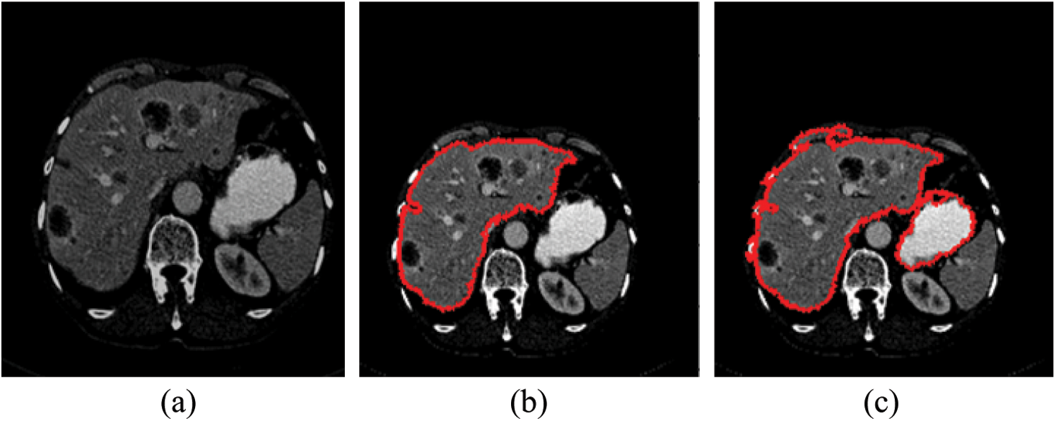
Figure 3: Liver segmentation (a) Enhanced abdomen image, (b) Liver segmentation using FGFCM, (c) Liver segmentation using FCM

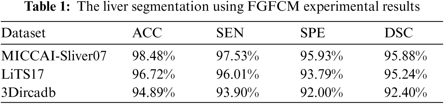
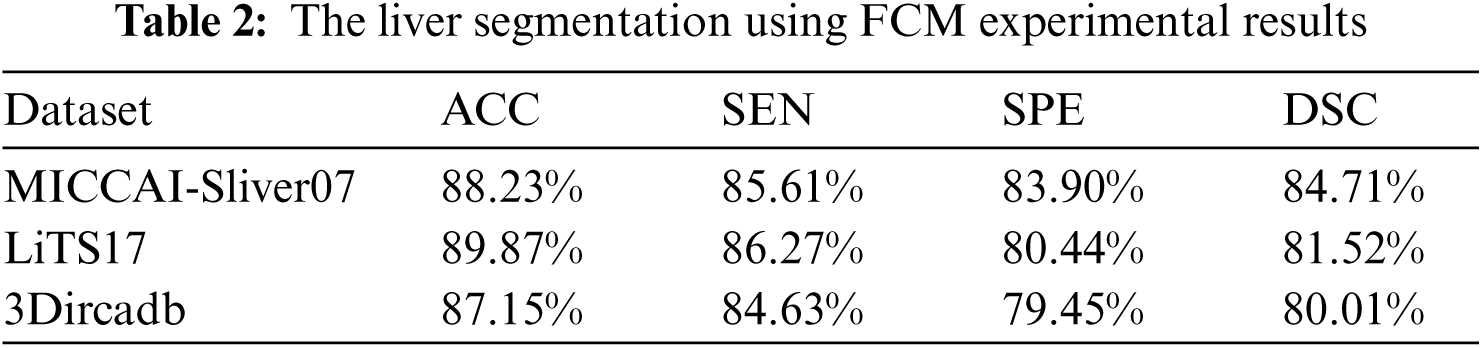
According to Tabs. 1 and 2, FGFCM results in more accurate and reliable segmentation when compared to the original FCM. The mean segmentation accuracy, sensitivity, and specificity were improved by almost 8%, 10%, and 12% respectively when the FGFCM was the segmentation method. This improvement is the consequence of considering pixels’ spatial and grey-level local correlations in the membership function and low noise sensitivity and detail preserving abilities. To reduce the segmentation time, FGFCM reduces the complexity of the segmentation process. This can be achieved by considering the total number of grey levels on the CT scan rather than the size of the scan. The proposed CAD system doesn't require user interaction to identify the trade-off between efficiency and noise suppression. This proves the reliability and automation of the proposed method.

Tumor segmentation experiment was implanted 3Dircadb and LiTS17 datasets only. This because MICCAI-Sliver07 dataset is mainly concerned with the liver segmentation and doesn't include tumors nor their GT. The experimental results for tumor segmentation are demonstrated by Tab. 3. The results in Tab. 3 show that the proposed CAD system achieved high segmentation accuracy for tumor segmentation from CT scans. Fig. 4 illustrates the tumors segmentation from the segmented liver.

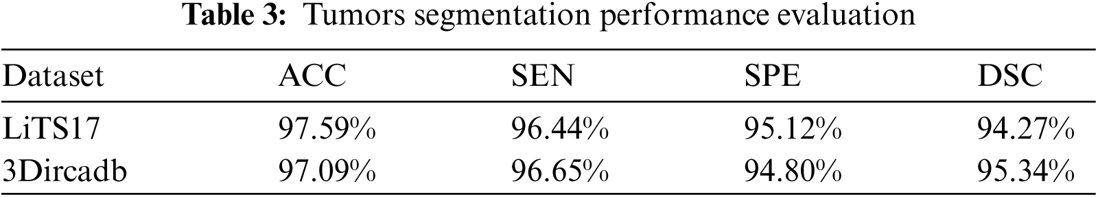
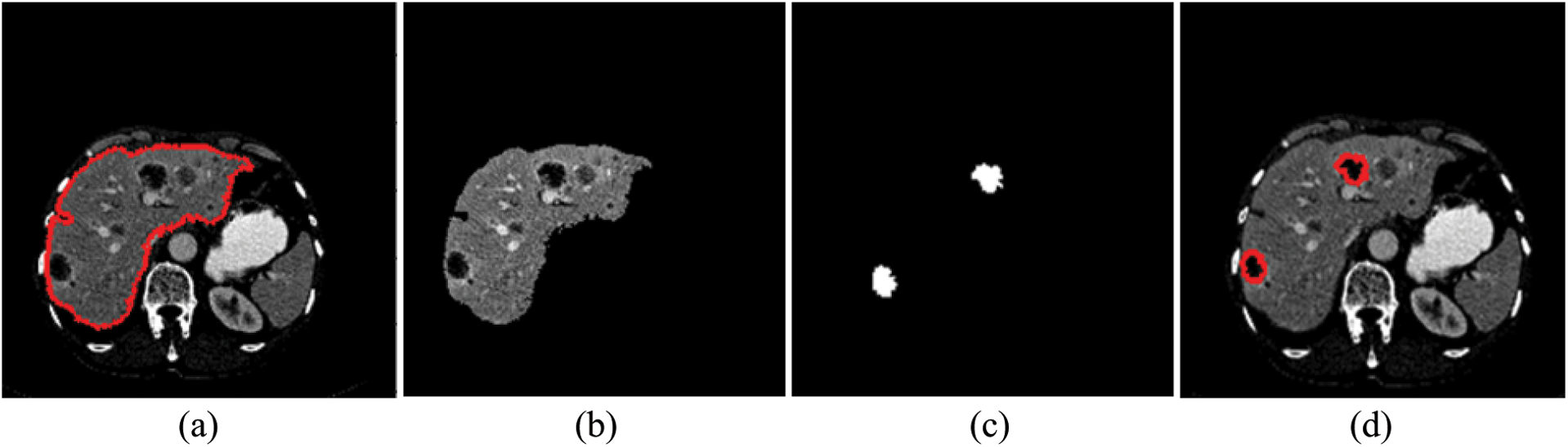
Figure 4: The experimental results of the segmntation processes (a) Outlined liver, (b) Segmented liver using FGFCM, (c) Outlined tumors and (d) Segmented tumors binary masks

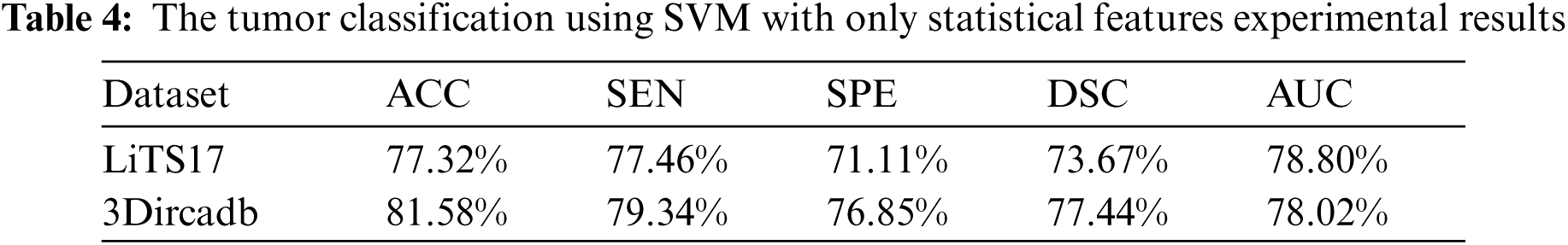
The tumor classification process was implemented in terms of statistical features only. Besides, it was implemented in terms of statistical and textural features using the SVM classifier. As illustrated in Tab. 4, statistical features fail to characterize tumors well. When those features were combined with textural features, they succeeded in characterizing the detected tumors and helped in raising the accuracy for labeling tumors as either malignant or benign.

The proposed system used mean, standard deviation, skewness as statistical features, and GLDM as textural features. Tab. 5 showed the experimental results for tumor classification when statistical and textural features were combined. Fig. 5 shows the ROC curves for classification with statistical features only and with statistical and textural features combined.

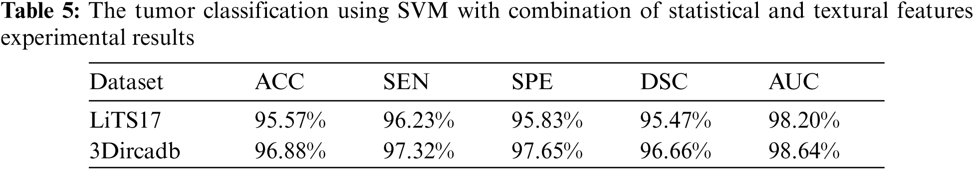
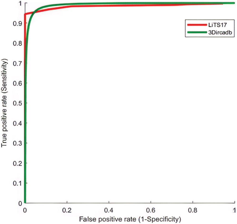
Figure 5: The ROC curve for tumors classification using statistical and textural features

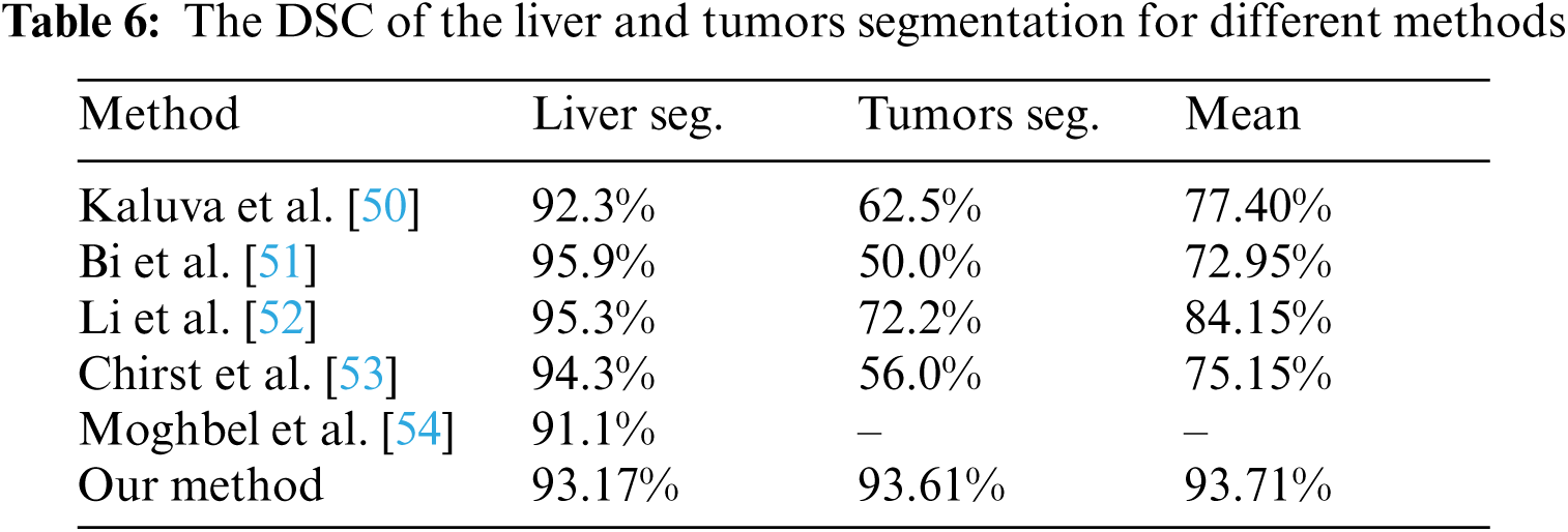
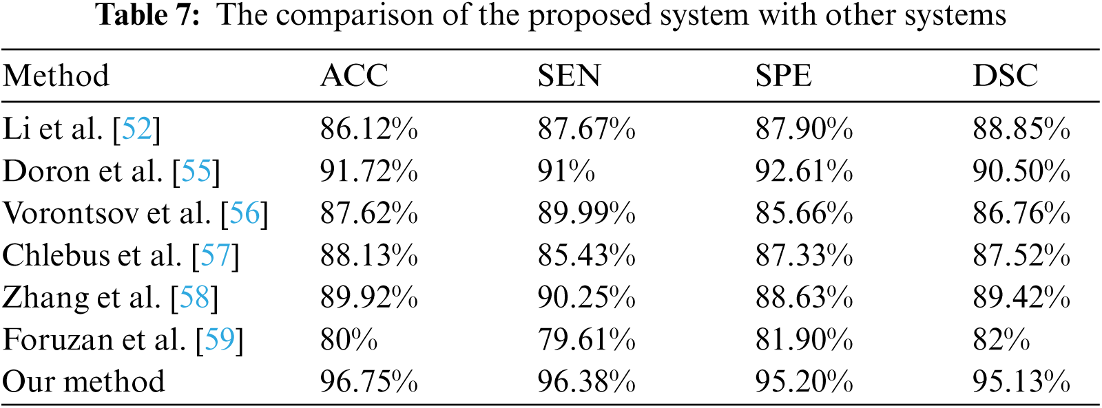
The performance of the proposed method was evaluated in comparison with other related studies which evaluated their work using MICCAI-Sliver07, 3Dircadb, or LiTS17 datasets. The average DSC results of the proposed CAD system in terms of the liver and tumor segmentation are listed in Tab. 6. The overall performance of the CAD system in comparison with other CAD systems is demonstrated in Tab. 7. The experimental results in Tabs. 6 and 7 prove the superiority and applicability of the proposed CAD system.

The liver segmentation task from CT scans is considered a very challenging and complicated task due to various factors. First, the liver has high intensities values overlap with its neighboring organs. Second, CT scans are highly affected by the impulse noises imposed by the CT scanner. Last but not least, the segmentation methods have high noise sensitivity. As a result of all those factors, the segmentation quality decreases resulting in under or over segmentation and the segmentation method will fial to correctly contour the ROI. They may also consume long processing time due to the noise.

The proposed CAD system used AMF with contrast enhancement technique as a pre-segmentation stage to reduce the noise effect. Besides, FGFCM was used as actual liver segmentation since it had high noise robustness, details preserving abilities with low complixty implemmtation. FGFCM resulted in high quality segmentation because of two factors. First, the FGFCM algorithm consider the spatial relationship between CT scans pixels. Second, the usage of color mapping, AHE and AMF to enhance the quality of the scans. The processing complexity was much reduced by selecting CT scans where the liver can be differentiated and using them for further processing.

Luo et al. [60] segmented liver using discrete wavelet transform (DWT) with a sensitivity of 94.1%, but their method suffered from being relatively complex due to DWT coefficients computations. Hameed et al. [61] proposed a CAD system to classify CT scans liver tumors into either malignant or benign. This method was unable to deal with high-order features and resulted in a sensitivity of 84%. Chen et al. [62] proposed a CAD system to diagnose hepatic cirrhosis tumors. This method achieved abnormal tumors diagnosis accuracy of 90% but failed to deal with large datasets. Edwin et al. [63] proposed an enhanced tumor segmentation method based on the thresholding approach. Their method achieved 93% sensitivity but suffered from over/under segmentation with complexity in threshold value selection. Das et al. [64] proposed an automatic CAD system to diagnose tumors using adaptive thresholding and achieved 89.15% accuracy. The proposed CAD system achieved an average ACC of 96.75%, SEN of 96.38%, SPE of 95.20% and DSC of 95.13%. It had the advantage of being fully automatic and robust to noise. It was also able to achive low complexity implementation by being implemented using CT scans at which liver can be differentiated and discarding those slices with heart or other abdomen organs. Our CAD system could deal with large datasets and was verified using three benchmark datasets, 3Dircadb, LiTS17, and MICCAI-Sliver07, with total cases of 250 subjects.

We developed a new CAD system that can be applied to different datasets to diagnose malignant and benign liver tumors from CT scans. We used three different public datasets, MICCAI-Sliver07, LiTS17, and 3Dircad. The proposed system starts by selecting CT slices based on liver clarity. Then, it enhances the quality of CT scans using filtering and contrast enhancement techniques. Next, the preprocessed CT scans are segmented into liver and abdomen regions using the FGFCM algorithm. Then, the segmented liver is passed as input to the OTZU thresholding method to segment tumor regions. After that, the system extracts four features which are the combination of textural and statistical features. Finally, the extracted features are passed to SVM to label tumors as either malignant or benign. To validate the proposed system, different performance metrics were calculated. The proposed CAD system achieved an average ACC of 96.75%, SEN of 96.38%, SPE of 95.20% and DSC of 95.13%. In the future, we are focusing on incorporating artificial intelligence techniques into our method, providing classification method that can label detected tumors into more sophisticated classes such as HCC and Cyst, enhancing the tumor classification process by using more features that can best characterize each type of liver tumors while maintaining low computational time. In future, we are focusing on incorporating artificial intelligence techniques into our method, providing classification method that can label detected tumors into more sophisticated classes such as HCC and Cyst, enhancing tumor classification process by using more features that can best characterize liver tumors with lower computational time, providing segmentation methods that can handle features with high order and building our own dataset and using it for our implementations.

Conflicts of Interest: The authors declare that they have no conflicts of interest to report regarding the present study.

References

J. Seco, B. Clasie and M. Partridge, “Review on the characteristics of radiation detectors for dosimetry and imaging,” Physics in Medicine and Biology, vol. 59, no. 20, pp. R303–R347, 2014.
R. Sharma, “Descriptive epidemiology of incidence and mortality of primary liver cancer in 185 countries: Evidence from GLOBOCAN 2018,” Japanese Journal of Clinical Oncology, vol. 50, no. 12, pp. 1370–1379, 2020.
T. Kogiso and K. Tokushige, “The current view of nonalcoholic fatty liver disease-related hepatocellular carcinoma,” Cancers, vol. 13, no. 3, pp. 516, 2021.
Y. N. Zhang, K. J. Fowler, G. Hamilton, J. Y. Cui, E. Z. Sy et al., “Liver fat imaging—a clinical overview of ultrasound, CT, and MR imaging,” The British Journal of Radiology, vol. 91, pp. 20170959, 2018.
S. S. Gunasundari and M. S. Ananthi, “Comparison and evaluation of methods for liver tumor classification from CT datasets,” International Journal of Computer Applications, vol. 39, no. 18, pp. 46–51, 2012.
G. Li, X. Chen, F. Shi, W. Zhu, J. Tian et al., “Automatic liver segmentation based on shape constraints and deformable graph cut in CT images,” IEEE Transactions on Image Processing, vol. 24, no. 12, pp. 5315–5329, 2015.
E. -L. Chen, P. -C. Chung, C. -L. Chen, H. -M. Tsai and C. -I. Chang, “An automatic diagnostic system for CT liver image classification,” IEEE Transactions on Biomedical Engineering, vol. 45, no. 6, pp. 783–794, 1998.
C. -L. Ho, S. Chen, D. W. Yeung and T. K. Cheng, “Dual tracer PET/CT imaging in evaluation of metastatic hepatocellular carcinoma,” Journal of Nuclear Medicine, vol. 48, no. 6, pp. 902–909, 2007.
R. L. Schapiro and L. C. Chiu, “Computed tomography of the liver: A review,” Journal of Computed Tomography, vol. 2, no. 4, pp. 331–341, 1978.
L. Xie, Y. Guang, H. Ding, A. Cai and Y. Huang, “Diagnostic value of contrast enhanced ultrasound, computed tomography and magnetic resonance imaging for focal liver lesions: A meta-analysis,” Ultrasound in Medicine & Biology, vol. 37, no. 6, pp. 854–861, 2011.
B. Blechacz and G. J. Gores, “Positron emission tomography scan for a hepatic mass,” Hepatology, vol. 52, no. 6, pp. 2186–2191, 2010.
A. Ciurte and S. Nedevschi, “Texture analysis within contrast enhanced abdominal CT images,” in IEEE 5th Int. Conf. on Intelligent Computer Communication and Processing, Cluj-Napoca, Romania, pp. 73–78, 2009.
M. K. Santos, J. R. F. Júnior, D. T. Wada, A. P. M. Tenório, M. H. N. Barbosa et al., “Artificial intelligence, machine learning, computer-aided diagnosis, and radiomics: Advances in imaging towards to precision medicine,” Radiologia Brasileira, vol. 52, no. 6, pp. 387–396, 2019.
J. H. Moltz, L. Bornemann, V. Dicken and H. Peitgen, “Segmentation of liver metastases in ct scans by adaptive thresholding and morphological processing,” in Proc. of MICCAI Workshop, Berlin, Germany, pp. 1–8, 2008.
C. Huang, F. Jia, Y. Li, X. Zhang, H. Luo et al., “Fully automatic liver segmentation using probability atlas registration,” in Int. Conf. on Electronics, Communications and Control, Zhoushan, Zhejiang, China, pp. 126–129, 2012.
D. Wong, J. Liu, Y. Fengshou, Q. Tian, W. Xiong et al., “A semi-automated method for liver tumor segmentation based on 2d region growing with knowledge-based constraints,” in Proc. of MICCAI Workshop, Berlin, Germany, pp. 1–10, 2008.
R. Pohle and K. D. Toennies, “Segmentation of medical images using adaptive region growing,” in Proc. of SPIE Medical Imaging, San Diego, California, USA, pp. 1337–1346, 2001.
B. N. Li, C. K. Chui, S. H. Ong and S. Chang, “Integrating FCM and level sets for liver tumor segmentation,” in Proc. 13th Int. Conf. on Biomedical Engineering, Berlin, Germany, pp. 202–205, 2008.
J. -Y. Zhou, D. W. K. Wong, F. Ding, S. K. Venkatesh, Q. Tian et al., “Liver tumour segmentation using contrast-enhanced multi-detector CT data: Performance benchmarking of three semiautomated methods,” European Radiology, vol. 20, no. 7, pp. 1738–1748, 2010.
N. H. Abdel-Massieh, M. M. Hadhoud and K. M. Amin, “Automatic liver tumor segmentation from CT scans with knowledge-based constraints,” in Cairo Int. Biomedical Engineering Conf., Cairo, Egypt, pp. 215–218, 2010.
S. S. Kumar, R. S. Moni and J. Rajeesh, “Automatic liver and lesion segmentation: A primary step in diagnosis of liver diseases,” Signal, Image and Video Processing, vol. 7, no. 1, pp. 163–172, 2011.
Y. Zhao, Y. Zan, X. Wang and G. Li, “Fuzzy C-means clustering-based multilayer perceptron neural network for liver CT images automatic segmentation,” in 2010 Chinese Control and Decision Conf., Xuzhou, China, pp. 3423–3427, 2010.
M. Danciu, M. Gordan, C. Florea and A. Vlaicu, “3D DCT supervised segmentation applied on liver volumes,” in 5th Int. Conf. on Telecommunications and Signal Processing, Roma, Italy, pp. 779–783, 2012.
H. Ji, J. He, X. Yang, R. Deklerck and J. Cornelis, “ACM-Based automatic liver segmentation from 3D CT images by combining multiple atlases and improved mean-shift techniques,” IEEE Journal of Biomedical and Health Informatics, vol. 17, no. 3, pp. 690–698, 2013.
D. Smeets, D. Loeckx, B. Stijnen, B. D. Dobbelaer, D. Vandermeulen et al., “Semi-automatic level set segmentation of liver tumors combining a spiral-scanning technique with supervised fuzzy pixel classification,” Medical Image Analysis, vol. 14, no. 1, pp. 13–20, 2010.
A. Moghe, D. J. Singhai and D. S. Shrivastava, “Automatic threshold-based liver lesion segmentation in abdominal 2d ct images,” International Journal of Image Processing, vol. 5, no. 2, pp. 166–176, 2011.
W. N. Yussof and H. Burkhardt, “3D volumetric CT liver segmentation using hybrid segmentation techniques,” in Int. Conf. of Soft Computing and Pattern Recognition, Malacca, Malaysia, pp. 85, 2009.
Y. Hame, “Liver segmentation using implicit surface evaluation,” in Medical Image Computing and Computer-Assisted Intervention-MICCAI 2008, vol. 2, New York, USA, pp. 1–10, 2008.
A. Adcock, D. Rubin and G. Carlsson, “Classification of hepatic lesions using the matching metric,” Computer Vision and Image Understanding, vol. 121, pp. 36–42, 2014.
W. Huang, N. Li, Z. Lin, G. B. Huang, W. Zong et al., “Liver tumor detection and segmentation using kernel-based extreme learning machine,” in Annual Int. Conf. of the IEEE Engineering in Medicine and Biology Society (EMBC), Osaka, Japan, pp. 3662–3665, 2013.
B. N. Li, C. K. Chui, S. Chang and S. H. Ong, “A new unified level set method for semi-automatic liver tumor segmentation on contrast-enhanced CT images,” Expert Systems with Applications, vol. 39, no. 10, pp. 9661–9668, 2012.
G. Mariani, L. Bruselli, T. Kuwert, E. E. Kim, A. Flotats et al., “A review on the clinical uses of SPECT/CT,” European Journal of Nuclear Medicine and Molecular Imaging, vol. 37, no. 10, pp. 1959–1985, 2010.
B. Van Ginneken, T. Heimann and M. Styner, “3D segmentation in the clinic: A grand challenge,” in MICCAI Workshop on 3D Segmentation in the Clinic: A Grand Challenge, Brisbane, Australia, pp. 7–15, 2007.
L. Soler, A. Hostettler, V. Agnus, A. Charnoz, J. Fasquel et al., “3D image reconstruction for comparison of algorithm database: A patient specific anatomical and medical image database,” IRCAD, Strasbourg, France, Tech. Rep,, 2010.
P. Bilic, P. F. Christ, E. Vorontsov, G. Chlebus, H. Chen et al., “The liver tumor segmentation benchmark (lits),” Computer Vision and Pattern Recognition, vol. 1901, pp. 40–83, 2019.
T. Razi, P. Emamverdizadeh, N. Nilavar and S. Razi, “Comparison of the hounsfield unit in CT scan with the gray level in cone-beam CT,” Journal of Dental Research, Dental Clinics, Dental Prospects, vol. 13, no. 3, pp. 177–182, 2019.
M. Kumar and A. Rana, “Image enhancement using contrast limited adaptive histogram equalization and wiener filter,” International Journal of Engineering and Computer Science, vol. 5, no. 6, pp. 2225–2231, 2016.
C. Y. Ning, S. F. Liu and M. Qu, “Research on removing noise in medical image based on median filter method,” in IEEE Int. Symposium on IT in Medicine & Education, Jinan, Shandong, China, pp. 384–388, 2009.
J. C. Bezdek, R. Ehrlich and W. Full, “FCM: The fuzzy c-means clustering algorithm,” Computers & Geosciences, vol. 10, no. 2–3, pp. 191–203, 1984.
S. Chen and D. Zhang, “Robust image segmentation using FCM with spatial constraints based on new kernel-induced distance measure,” IEEE Transactions on Systems, Man and Cybernetics, Part B (Cybernetics), vol. 34, no. 4, pp. 1907–1916, 2004.
W. Cai, S. Chen and D. Zhang, “Fast and robust fuzzy c-means clustering algorithms incorporating local information for image segmentation,” Pattern Recognition, vol. 40, no. 3, pp. 825–838, 2007.
N. Otsu, “A threshold selection method from gray-level histograms,” IEEE Transactions on Systems, Man, and Cybernetics, vol. 9, no. 1, pp. 62–66, 1979.
T. Moser and T. S. Nogueira, “Localized fibrous tumor of the liver: Imaging features,” Liver Cancer, vol. 5, pp. 17–19, 2009.
D. Giosa, F. C. D. Tocco, G. Raffa, C. Musolino, D. Lombardo et al., “Comprehensive characterization of HBV in tumor and non-tumor liver tissues from patients with HBV related-HCC,” Digestive and Liver Disease, vol. 52, pp. e3–e4, 2020.
A. H. AB, S. A. Ahmed, M. E. M. Gar-elnabi, M. A. Omer and A. I. Ahmed, “Characterization of hepatocellular carcinoma (HCC) in CT images using texture analysis technique,” International Journal of Science and Research (IJSR), vol. 5, no. 1, pp. 917–921, 2016.
W. Schima, D. M. Koh. and R. Baron, “Focal liver lesions,” in Diseases of the Abdomen and Pelvis 2018–2021, Milano, Italy, Springer, 17, pp. 95–110, 2018.
T. S. Furey, N. Cristianini, N. Duffy, D. W. Bednarski, M. Schummeret et al., “Support vector machine classification and validation of cancer tissue samples using microarray expression data,” Bioinformatics, vol. 16, no. 10, pp. 906–914, 2000.
M. A. Nanda, K. B. Seminar, D. Nandikaand A. Maddu, “A comparison study of kernel functions in the support vector machine and its application for termite detection,” Information, vol. 9, no. 1, pp. 5, 2018.
A. U. Haq, J. P. Li, A. Saboor, J. Khan, S. Wali et al., “Detection of breast cancer through clinical data using supervised and unsupervised feature selection techniques,” IEEE Access, vol. 9, pp. 22090–22105, 2021.
K. C. Kaluva, M. Khened, A. Kori and G. Krishnamurthi, “2D-densely connected convolution neural networks for automatic liver and tumor segmentation,” Computer Vision and Pattern Recognition, vol. 1802, pp. 18–21, 2018.
L. Bi, J. Kim, A. Kumar and D. Feng, “Automatic liver lesion detection using cascaded deep residual networks,” Computer Vision and Pattern Recognition, vol. 1704, pp. 21–27, 2017.
X. Li, H. Chen, X. Qi, Q. Dou, C. -W. Fu et al., “H-DenseUNet: Hybrid densely connected UNet for liver and tumor segmentation from CT volumes,” IEEE Transactions on Medical Imaging, vol. 37, no. 12, pp. 2663–2674, 2018.
P. F. Christ, F. Ettlinger, F. Grün, M. E. A. Elshaera, J. Lipkova et al., “Automatic liver and tumor segmentation of CT and MRI volumes using cascaded fully convolutional neural networks,” Computer Vision and Pattern Recognition, vol. 1702, pp. 59–70, 2017.
M. Moghbel, S. Mashohor, R. Mahmud and M. I. B. Saripan, “Automatic liver tumor segmentation on computed tomography for patient treatment planning and monitoring,” EXCLI Journal, vol. 15, pp. 406–423, 2016.
Y. Doron, N. Mayer-Wolf, I. Diamant and H. Greenspan, “Texture feature based liver lesion classification,” Medical Imaging 2014: Computer-Aided Diagnosis, vol. 9035, pp. 90353K, 2014.
E. Vorontsov, N. Abi-Jaoudeh and S. Kadoury, “Metastatic liver tumor segmentation using texture-based omni-directional deformable surface models,” in Int. MICCAI Workshop on Computational and Clinical Challenges in Abdominal Imaging, Cambridge, Massachusetts, USA, pp. 74–83, 2014.
G. Chlebus, A. Schenk, J. H. Moltz, B. V. Ginneken, H. K. Hahn et al., “Automatic liver tumor segmentation in CT with fully convolutional neural networks and object-based postprocessing,” Scientific Reports, vol. 8, no. 1, Computer Vision and Pattern Recognition, vol. 1901, pp. 1–7, 2018.
J. Zhang, Y. Xie, P. Zhang, H. Chen, Y. Xia et al., “Light-weight hybrid convolutional network for liver tumor segmentation,” in Proc. of the Twenty-Eighth Int. Joint Conf. on Artificial Intelligence, Macao, China, vol. 19, pp. 4271–4277, 2019.
A. H. Foruzan and Y. W. Chen, “Improved segmentation of low-contrast lesions using sigmoid edge model,” International Journal of Computer Assisted Radiology and Surgery, vol. 11, no. 7, pp. 1267–1283, 2015.
S. Luo, Q. Hu, X. He, J. Li, J. S. Jin et al., “Automatic liver parenchyma segmentation from abdominal CT images using support vector machines,” in 2009 ICME Int. Conf. on Complex Medical Engineering, Tempe, Arizona, USA, pp. 1–5, 2009.
R. Hameed and S. Kumar, “Assessment of neural network based classifiers to diagnose focal liver lesions using CT images,” Procedia Engineering, vol. 38, pp. 4048–4056, 2012.
Y. W. Chen, J. Luo, C. Dong, X. Han, T. Tateyama et al., “Computer-aided diagnosis and quantification of cirrhotic livers based on morphological analysis and machine learning,” Computational and Mathematical Methods in Medicine, vol. 2013, pp. 1–8, 2013.
D. Edwin and S. Hariharan, “Liver and tumour segmentation from abdominal CT images using adaptive threshold method,” International Journal of Biomedical Engineering and Technology, vol. 21, no. 2, pp. 190–204, 2016.
A. Das, P. Das, S. S. Panda and S. Sabut, “Detection of liver cancer using modified fuzzy clustering and decision tree classifier in CT images,” Pattern Recognition and Image Analysis, vol. 29, no. 2, pp. 201–211, 2019.

Computers, Materials & Continua DOI:10.32604/cmc.2022.023638
Article