DOI:10.32604/cmc.2022.023557
| Computers, Materials & Continua DOI:10.32604/cmc.2022.023557 | |
| Article |
Emotion Based Signal Enhancement Through Multisensory Integration Using Machine Learning
1Pattern Recognition and Machine Learning Lab, Department of Software, Gachon University, Seongnam, Gyeonggido, 13120, Korea
2Riphah School of Computing & Innovation, Faculty of Computing, Riphah International University Lahore Campus, Lahore, 54000, Pakistan
3School of Computer Science, National College of Business Administration and Economics, Lahore, 54000, Pakistan
4Department of Computer Engineering, Gachon University, Seongnam, 13557, Korea
*Corresponding Author: T. Whangbo. Email: tkwhangbo@gachon.ac.kr
Received: 12 September 2021; Accepted: 13 October 2021
Abstract: Progress in understanding multisensory integration in human have suggested researchers that the integration may result into the enhancement or depression of incoming signals. It is evident based on different psychological and behavioral experiments that stimuli coming from different perceptual modalities at the same time or from the same place, the signal having more strength under the influence of emotions effects the response accordingly. Current research in multisensory integration has not studied the effect of emotions despite its significance and natural influence in multisensory enhancement or depression. Therefore, there is a need to integrate the emotional state of the agent with incoming stimuli for signal enhancement or depression. In this study, two different neural network-based learning algorithms have been employed to learn the impact of emotions on signal enhancement or depression. It was observed that the performance of a proposed system for multisensory integration increases when emotion features were present during enhancement or depression of multisensory signals.
Keywords: Multisensory integration; sensory enhancement; depression; emotions
The brain is the most complex part of the human body. The nervous system inside the human brain is composed of different types of cells. The primary functional unit of the nervous system is called the neuron. Every neuron passes signals which cause thoughts, actions, feelings, and memories [1]. The brain has a specific area to deal with sensory input and the most significant capabilities of the brain include an appropriate response to sensory input and information processing [2]. The human brain has the great capability to perceive the information of the outer world through various sensors, process this information, and generate a response accordingly [3]. Recently several attempts have been made to simulate these functions of the brain into cognitive agents [2,4,5].
The cognitive agents are the systems that sense the environment from time to time and generate appropriate actions, in pursuit of their agenda [4,5]. Most of the cognitive agents are not able to perform multisensory integration or either they do not deal with the sensory data efficiently received from multiple sensors. The integration of multiple sensory data may result in the enhancement or depression of incoming signals [6,7]. Enhancement and depression of different sensory stimuli is a very significant characteristic of multisensory integration [8]. Interactions in the multisensory environment are normally restrained by the primary unimodal stimuli therefore the role of secondary auditory input is to enhance the response of multisensory integration to non-perceived visual inputs [8].
When different sensors observe the same event, multiple questions arise that upon receiving multiple measurements of a single event, how consistent perception is generated by the system with higher accuracy [9–11]. Another important question that may arise is, that, how optimal decisions are made by the systems when various perceptions are measured through different sensors [12,13]. Although every sensor has its congenital deficiencies and margins, yet the redundant data sensed through different sensors is fused to provide precise and accurate perception due to the sensory enhancement and depression phenomenon [1,7]. The system may produce a more accurate and reliable decision by diminishing the perceptual uncertainty through this phenomenon [11,14]. All cognitive agents are considered to perform optimally in integration tasks particularly in enhancement and depression in a way that they take uncertainty into account to integrate information coming from different sources [15]. It is important to elucidate that how neurons can produce such optimal probabilistic inference based on sensory representation considering the structure of the brain [16]. It is also significant to study how neural networks can acquire the knowledge about their environment that is the base of such computations [8,13].
Studies on human emotion recognition typically use facial expressions and emotional voice expressions which appear to be the most complex visual and auditory stimuli [14,15]. The vocal stimuli of emotions may affect the perception of facial expression in a way that people may visualize the felt textures or may feel touched by visualizing textures [15,16]. Although data are not directly useful to understand how and when both the face and the voice are present, yet the two information streams are integrated [17,18]. Multisensory integration contributes to a sense of self and an intensified presence of the perceiver in his or her world [19]. This aspect of multisensory integration is particularly relevant for the multisensory perception of emotion [20]. A comprehensive computational methodology is being proposed in this research paper, with the intent of understanding the functional features and advantages of emotions for multisensory enhancement and depression phenomenon. The prime focus of this research is to observe the orientation of integrated incoming stimuli for enhancement and depression criteria with the assumption that both the stimuli appear concurrently in Superior colliculus (SC) along with emotions. This research paper provides the basics to understand the impact of emotions in multisensory enhancement and depression to design a model for cognitive agents which may generate more appropriate responses while interacting in dynamic environments. In forthcoming sections, a brief review of literature is presented to outline the work done so far, then the proposed methodology is described with results and outcomes.
Research in neuroscience and cognitive sciences have studied sensory enhancement and depression phenomenon in humans and animals in great detail. Stein [8,21] demonstrated visual enhancement based on the neurophysiological phenomenon first time through integrative processing of multisensory stimuli in nonhuman species. A very significant characteristic of multisensory integration is the foundation of enhancement of visual stimuli. Interactions in the multisensory environment are normally restrained by the primary unimodal stimuli so the role of secondary auditory input is to enhance the response of multisensory integration to non-perceived visual inputs [8].
In recent years, the advantages of multisensory integration have also inspired research in different applications areas [14]. Expendable and complementary sensory data that come from different sensory systems can be integrated using different multisensory integration methods to increase the capability of the agent [22–24]. To use sensory data in the integration process, it needs to be effectively modeled. The sensors model epitomizes the errors and uncertainty in the sensory data and measures the quality of sensory data that can be used in subsequent integration functions [20]. After modeling this sensory data, the processing may result into following three different types of processing stages: fusion, separate operation, and guiding or cueing [25–27]. It is also a possible research area to understand when and how the human brain decides to opt between fusion, separation, and cueing [28].
Events that happen in the external environment are more simply perceived and localized when cross-modal stimuli being initiated from a similar location. The neuronal responses generated by SC are enhanced at the physiological level when stimuli coming from different modalities descent into the relevant receiving fields of overlapping unisensory neurons [9,29]. Similarly, the responses of SC and accuracy of localization should be depressed when the same stimuli are originated from different places or descent into receptive fields of neurons surrounding inhibitory regions [30,31]. Another significant point to note is that the localization of visual stimulus does not depress when a blurred or vague visual target is collectively analyzed with auditory stimuli placed in exterior space [27]. It has also been observed during various psychological and behavioral studies of humans and animals that upon receiving diverse strengths of dissimilar stimuli coming from different perceptual modalities at the same time or from the same place, the signal having more strength effects the response accordingly [6,32,33].
Multisensory enhancement and depression are primarily based on the space between different perceptual stimuli and the strength of incoming stimuli [34,35]. It is believed by many researchers that SC takes into account the significance of primary visual stimuli because of its straight interaction with visual sensors through vision sensors. This phenomenon occurs only when stimuli are observed having different strengths at varied time intervals [1,36–38]. For example, if any human agent is sitting on a revolving chair and the chair is rotated several times, finally when that chair will stop, the received visual stimulus will be superseded by an acoustic stimulus received through the ear [37,38]. It can be noticed that initially the optical stimulus is superseded by the acoustic stimulus, but at further stages, the acoustic stimulus will also lose effectively when it tries to integrate visual and audio stimuli. It happens because of the ever-changing state of sensors (in this case eyes and ears) [39]. This scenario implies the fact that both the stimuli (eyes and ears) are equally prioritized during the integration process yet for signal enhancement and depression, both stimuli may be treated differently [37].
In multisensory enhancement when strong and weak perceptual stimuli are received then the stronger perceptual stimuli can be enhanced [40]. When some strong and reasonably similar perceptual stimuli are received, it will more likely have resulted in enhancement of unified or integrated signal instead of enhancement of individual stimulus. Likewise, when two weak and relatively closer perceptual stimuli are received the enhancement may occur in the integrated output of either or both of the received stimuli [37,41]. Depression is the phenomenon in which the current state of the agent is reported as misperception [42]. This misperception arises while determining the angle for localization [43] particularly in cases when some strong perceptual stimuli are perceptually dissimilar from each other, in such a scenario the output will be more depressed. Similarly, if the two weak perceptual stimuli that are far away from one another being received then the output will again be strongly depressed, resulting in that no output will be generated [44]. Multisensory enhancement, on the other hand, may improve the ability of an organism to detect the targets in the environment. Deep & Machine learning arose over the last two decades from the increasing capacity of computers to process large amounts of data. Machine learning approaches like Swarm Intelligence [45], Evolutionary Computing [46] like Genetic Algorithm [47], Neural Network [48], Deep Extreme Machine learning [49] and Fuzzy system [50–56] are strong candidate solution in the field of smart city [57–59], smart health [60,61], and wireless communication [62,63], etc.
This research paper is focused to develop a framework to study the impact of emotion on the enhancement and depression phenomenon of integrated signals in machines. This study allows the functionally cognitive agents to integrate multisensory stimuli on the most salient features of the sensed audio-visual information by considering internal and external psychophysical states for sensory enhancement or depression. The system model is illustrated in Fig. 1 as a solution to achieve multisensory integration for functional cognitive agents however the scope of this paper is limited to the multisensory enhancement and depression module of a proposed system model. Various components of the proposed model are capsulated and operate within the scope of a different interconnected cognitive subsystem. The model is given in Fig. 1 consist of four different modules, i.e., Sensory system (SS) to sense different stimuli from the environment, Perceptual associative memory (PAM) to perceive important information from sensory input, Working memory (WM) is a preconscious buffer and Emotion System (ES) to analyze and generate an emotional state of the system, given the sensory input. The focus of this research paper is limited to sensory enhancement or depression, other parts of SC such as the sensory integration module, event history module, and WM have been described in this paper very briefly to outline the scope of the generic system proposed for multisensory integration but they have no significance in this paper.
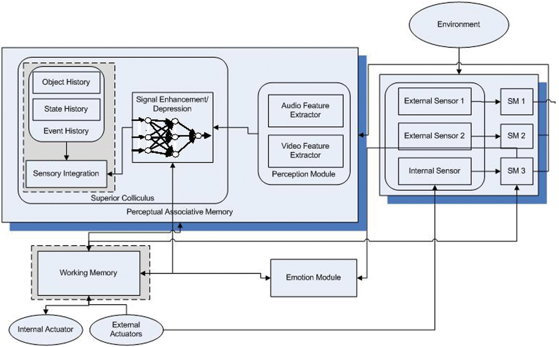
Figure 1: System model for emotion-based sensory enhancement and depression during multisensory integration using artificial neural networks
The sensory system is subdivided into internal and external sensors. The internal sensor senses the emotional states of conscious agents while the two external sensors sense audio and visual stimuli. These sensors transfer data to the sensory buffer temporarily for further processing. This buffered information shifts towards perceptual associative memory, which is further divided into two sub-modules like perceptual module and superior colliculus. The superior colliculus module is responsible for signal enhancement and depression phenomenon to integrate multisensory stimuli.
The prime purpose of this research is to study the influence of emotions to enhance or depress multisensory inputs. These sensory inputs are being sensed through SS which is built with internal and external sensors. This module can receive information from different sensors and save it into sensory memory. Only auditory and visual sensors have been used in the proposed system to reduce the computational complexity of SS. These sensors receive the audio and visual stimuli and forward them to PAM for further processing. The role of the internal sensor is to sense the emotional state of the agent and this state is sent to the emotional module.
3.2 Perceptual Associative Memory (PAM)
The sensed input is transferred to PAM from sensory memory for further processing. PAM consists of two sub-modules, Perception module (PM) and Superior colliculus (SC).
PM perceives low-level features from input stimuli after receiving the input from sensory memories. Enhancement and depression of sensory stimuli primarily depend on the perception of these features. For instance, if the pitch and frequency of any audio stimuli are very high, the agent should depress these auditory features so that visual and other sensory modalities may be integrated with auditory signals. PM contains two sub-modules, which are the audio feature extractor and video feature extractor. The perceived information is transferred to the SC, where signals are enhanced or depressed if deemed necessary and finally integrated.
Feature extraction has a very important role in this study and its intent is to analyze raw sensory data to analyze important features from incoming stimuli. Audio feature extractor separates important and useful audio data including features like Frequency, Formant Value, Pitch, and Timbre value.
Frequency is the oscillations of sound waves, as measured in hertz (cycles per second). Frequency is not concerned with the vibrating object used to create the sound wave, rather the speed of the particles vibrating in a back and forth motion at a given rate is known as frequency. Fewer vibrations in any certain amount of time are normally difficult to be noticed by the human ear and hence require more effort to generate more attention. The frequency may be expressed in Eq. (1), as follows.
Here the symbol F represents frequency and the symbol p represents period which is the number of vibrations per second. It is important to relate that higher frequencies are inclined to be directional and generally dissipate the energy quickly. However, lower frequencies are likely to be multi-directional and it becomes hard to localize lower frequencies as compared to the higher frequencies.
The pitch depicts the subjective psycho-acoustical sensation of high and low tones. Pitch is normally defined as the perceptual property of acoustic reverberations that agrees to the organization of multiple sounds on a frequency-related scale. It is significant to note that pitch can only be measured in sounds having a clear and stable frequency to be differentiated from noise. The higher the frequency the higher will be pitch as shown below in Eq. (2).
Timbre is another perceptual quality of sound that differentiates between various acoustic constructions. Generally, timbre differentiates any particular acoustic impression from others even if the pitch or loudness of both sounds are similar. The intensity of sounds and their frequencies are considered important in any waveform of which the timbre is computed. For instance, if sounds having different frequencies 100, 300, and 500 hertz are taken into account and relative amplitudes of 10, 5, and 2.5 are fused to form a complex sound then the amplitude “a” of the waveform at any time t would be represented by following Eq. (3).
It will be easy to recognize this timbre and it will be well differentiable from other sounds having diverse amplitude and a basic frequency of 100 hertz.
A formant is a grouping of acoustic strength around a specific frequency in the sound wave. There could be multiple formants having different frequencies about one in each 1000 hertz. Every formant relates to a sound in the vocal tract. The strength of formants means more energy in the vocal stimuli. The vocal tract producing different sounds can be roughly considered as a pipe barred from one side. Because the vocal tract evolves in time to produce different sounds, spectral characterization of the voice signal will be also variant in time. This temporal evolution may be represented with a voice signal spectrogram as shown in Eq. (4).
It is clear from above Eq. (4) that there can be several formants calculated at each value of n where n represents the sequence number of the formant as represented as Tn, i.e., the second formant would be written as T2. In Eq. (4) v is the speed of sound which is 34000 cm/sec and L is the length of the vocal tube.
The visual feature extractor receives the visual signal as input in the form of frames from the visual sensory memory. After preprocessing of data to remove irrelevant features ready to process data is extracted and transmitted for further processing. Every image contains a lot of information, yet the scope of this research is limited with entropy, mean color, RMS, and correlation features.
Entropy in the analysis of visual stimuli is considered as a quantity describing the amount of information in any image that needs to be coded for compression of the image. This quantity can be low or high where Low entropy means that the concerned image contains a considerable amount of background of the same color. Subsequently, images having high entropy, are those which have highly cratered areas, having a considerable amount of contrast from one pixel to another.
Eq. (5) returns a scalar value which gives the entropy of any image
Mean color is the measurement of the color temperature of any object that radiates light of comparable color. Mean color is normally expressed in kelvins, using the symbol K, which is a unit of measure for absolute temperature. Eq. (7) illustrates the formula to calculate mean color where i and j represent current pixel and ck represents color while k ranges from 1 to 3 showing red, green, and blue color.
RMS is used for transforming images into numbers and get the results for analysis. The use of RMS is helpful to refine the images and to explore error detection. For instance, if two images are required to be compared to evaluate if they belong to the same event or not a de-noised image
Correlation is represented by the “correlation coefficient”, which ranges between −1 and + 1. A correlation coefficient is computed as
where,
Emotions are representations of feelings and can be sensed through the internal sensors of the agent. It is believed by many researchers [10,19,21] that internal emotions can play a vital role in multisensory enhancement and depression. Progress of research in the field of cognitive agents has led toward employing agents to perform various tasks in daily life. For this purpose, the agents need to interact with other agents/humans and so they need to keep track of their psychological and physical states. The role of emotions in action selection is very important and it may influence the perception of the outside environment. In this model, the role of the emotion module is to understand emotional cues from audio and visual data. Humans can express several primary and secondary emotions, but the scope of this study is concerned with only six basic emotions. Once the agent perceives emotion from incoming stimuli, it can generate its sentiments.
The expression of emotions is an important and dynamically changing phenomenon, particularly for human beings. The strategy used in this research for classification and analysis of facial emotion comprises three significant steps. First of all important region features and skin color is detected from incoming stimuli using the spatial filtering approach. The next step is to locate the position of facial features to be represented as a region of interest and the Bezier curve is created by using a feature map from the region of interest. Furthermore, the calibration of illumination is done in this step as an essential preprocessing criterion for precise recognition of facial expressions as mentioned in Eq. (10).
where
In Eqs. (11) and (12), the region and position of eyes and lips are extracted from the visual incoming stimuli. Eyes have multiple basic properties like symmetry so can easily be detected and transformed into an eye map as mentioned in Eq. (12).
Here α = 1.2 and β = 0.8 are the experimental values and are predefined while the range of
To analyze resemblance in the incoming stimuli for similarity comparison, the normalization of curve displacements is done. This normalization step regenerates each width of curves with a threshold value of 100 to maintain the aspect ratio. Distance
It is apparent from Eq. (13) that other feature points may also be used for distance calculation. The emotion on the face depends upon the distance between different focus points.
Extracting features from audio signals was a bit difficult task for selected videos containing music along with speech signals. Humans are capable of focusing on the person who is speaking to us, by ignoring the noise of the environment. Therefore the first step of extracting emotions from auditory input was to remove noise from incoming stimuli which require separate discussion and are not part of this paper. Once noise was removed and audio features were extracted from auditory stimuli, the Levenberg marquardt (LM) algorithm was used to train an artificial neural network for which the Berlin Database of Emotional Speech was used as a training dataset. This database consists of 500 utterances spoken by the different actors in happy, angry, sad, disgust, boredom, fear, and normal ways. These utterances are from 10 different actors and ten different texts in the German language. Around 50, 50 samples of each emotion were taken to create the dataset for training. After training and validation, 96% accuracy was obtained and this trained network was later used to extract emotions from our dataset.
The superior colliculus is the region in the mid-brain, where multimodal stimulus processing and integration of audio-visual stimuli takes place. SC consists of signal enhancement and depression module, history manager, and sensory integration module. The scope of this research paper is limited to signal enhancement and depression module, other modules have also been described very briefly to outline the scope of the proposed system model.
3.7 Enhancement and Depression Module
This module is responsible for enhancement and depression of incoming stimuli before integration of different sensory cues. Before actually integrating different sensory inputs they are synchronized so that all sensory stimuli may get similar attention and so appropriate responses may be generated. In case the enhancement or depression phenomenon is not employed in the system, then the situation becomes more like of winner take all and so the sensor having more intense features in incoming stimuli will get whole attention and other sensors may not get proper attention resulting in inappropriate actions and responses. In this module, we are using artificial neural networks to train the system as to how and when to enhance or depress incoming stimuli. Two different learning methods have been used to train the system which are LM and Scaled Conjugate Gradient.
The LM algorithm is developed to work with loss functions that are formulated as the sum of squared errors. LM algorithm utilizes gradient vector and Jacobian matrix which maximizes the speed of training neural networks. Though this algorithm has limitations that for very big data sets the size of the jacobian matrix becomes large, and requires a lot of memory but for medium-size datasets it can work well. The main notion behind the LM algorithm is that the training process consists of two steps. The first step of the LM algorithm is that it changes to the steepest descent algorithm around an intricate curve until the local curve is appropriate to generate a quadratic approximation. The second step is to significantly speed up the convergence which makes it quite similar to the Gauss-Newton algorithm.
For the derivation of the LM algorithm in the aforementioned computation, the variables j and k are being used as the indices of neurons which range from 1 to any number nn, where nn is the number of neurons used in any neural network topology. The value of i which represents the index of input neurons ranges from 1 to j, the number of input neurons may always vary depending on the feature set provided in the data. For training of the neural network suppose there is input neuron j with ni inputs. As neuron j represents the input neuron, it will always exist in the first layer of network topology and all inputs of neuron j will be linked to the inputs of the network. Node
where
And slope
There is a complex non-linear relationship between the output of the network
The complexity of this nonlinear function
where the derived non-linear function
where,
The δ parameter in the LM algorithm is computed separately for every neuron j and every output m, and the computed error is replaced by a unit value during the backpropagation process as shown in Eq. (22).
The elements of the jacobian matrix can finally be computed by Eq. (23).
In case, the incoming stimuli match with stored signals, the history manager will generate a strong signal to integrate incoming stimuli according to already stored experiences. The history manager not only recognizes the individual objects rather it also manages the state of the objects with relevant details of the event.
Once processing is completed, all audiovisual signals are combined in the integration module. The input to this module has information regarding the direction of a person, its’ identity, and emotional state. The purpose of this module is to associate these heterogeneous signals coherently. The resultant output contains a unified, maneuvering, and affective signal carrying all relevant information about the objects.
After integration, input stimuli being integrated and transferred to working memory. WM provides temporary storage while manipulating information needed for understanding, learning, and reasoning for the current environment. Information comes into the working memory from two different sources. One source is the perceptual associative memory were initially integrated information is passed to working memory and the other source is the internal sensory memory from where the emotional state of the agent is transferred to WM. The signal from WM is further transferred to actuators to perform an action and the same signal is transferred to internal sensors through internal actuators.
In this paper, it is hypothesized based on the literature survey (as discussed in Section 2 of this paper) that emotions play a significant role in multisensory enhancement or depression during the sensory integration process in the superior colliculus. This behavior of the machine is able not only to integrate multi-sensory input but also mimics biology both at neuron level and behavioral level. It becomes very crucial almost every time to have a sufficient amount of training data to train the neural network and to cover the full range of the network and secure the applicability of the network with sufficient statistical significance. For dataset preparation, Twenty (20) different videos collected from various movies and documentaries on diverse topics were used in the experiment. There were no particular selection criteria for these videos. Persons participating in these videos were of different age groups, including both males and females. Although persons performing different actions belonged to different ethnic backgrounds, yet all of them were communicating in the English language. All of the video clips were processed and regenerated to have an identical format with the standard duration of 30 s. All sorts of introductory titles and subtitles were removed during preprocessing. In the video dataset, we first separated audio from visual data, and then each video segment was converted into images. For each video, visual features were extracted. Similarly, the audio features were also extracted to prepare the dataset containing more than 10000 records. The data that is used for training, testing, and validation of the ANN is shown in Fig. 2.
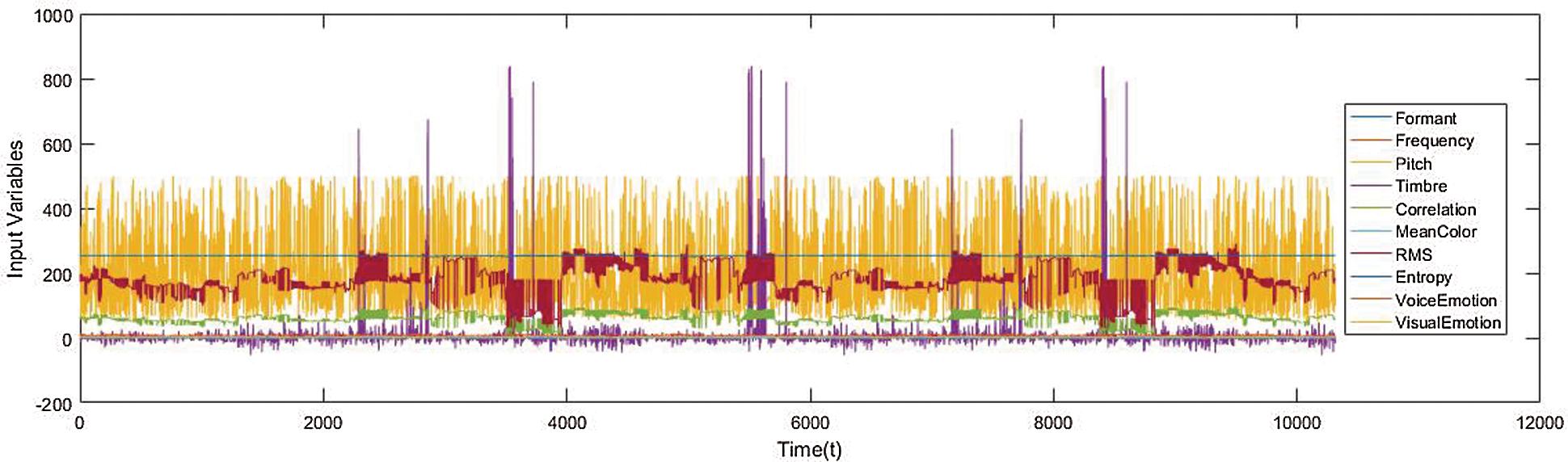
Figure 2: Features of the pre-generated dataset used for training, testing, and validation of ANN
In the design of the ANN architecture presented in Section 3.7, the results are obtained for an ANN trained with the MSE as an objective function or error measure. Thus, the various settings of the neural network are compared for the ANN with 10, 15, 20, and 25 neurons in the hidden layer in a different set of experiments, ten input variables representing different sensory features. The training length of the neural network was fixed at 1000 iterations but in most of the experiments, the network converged very early with good accuracy.
In every experiment, some of the pre-generated data were randomly selected for performance validation and testing of the trained neural network, and performance and regression graphs were saved for comparison. These data are used to calculate a validation error which is the measure for the accuracy of the trained network. Fig. 3 shows the development in the validation error during the network training with different settings of the hidden layer using pre-generated data set with emotion features. It is apparent from Fig. 3 that as the number of neurons in hidden layers are increases the performance of the system is also increased. Initially, the network was trained with 10 neurons in the hidden layer and the system converged in the 90th iteration while with 15 neurons in the hidden layer and the system converged earlier approximately in iteration 48 with a significant decrease in error. When the number of neurons in the hidden layer increased to a certain number it was observed that though the system converged in the 70th iteration the mean error decreased to approximately
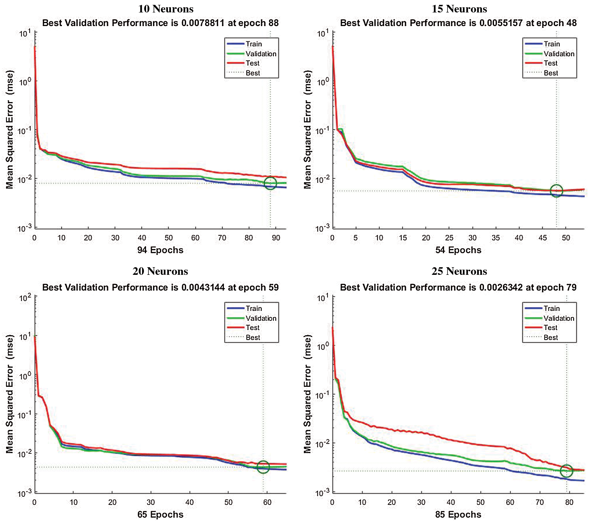
Figure 3: Performance of proposed system using LM algorithm with different number of neurons at hidden layer having emotion features
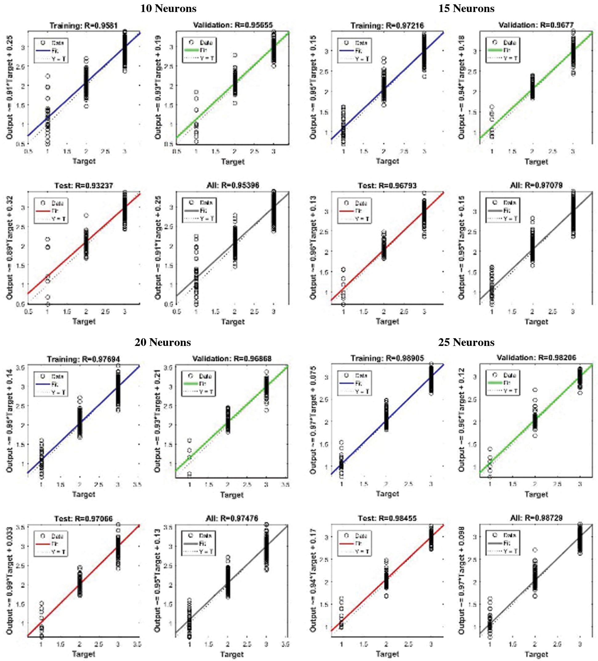
Figure 4: Regression comparison of proposed system using LM algorithm with different number of neurons at hidden layer having emotion features
In another set of experiments, the same pre-generated dataset was trained with other ANN algorithms but a significant decrease in performance was observed. Fig. 5 summarizes the development of the performance using scaled conjugate gradient backpropagation ANN, with a similar network setting and the number of neurons in the hidden layer using the same MSE error measure to give a consistent basis for comparison. It was observed that when 10 neurons were used in the hidden layer for training the network converged in approximately 200 iterations as shown in Fig. 5a but the performance remained low as compared to the same number of neurons used in the hidden layer with LM algorithm (see Fig. 4a).
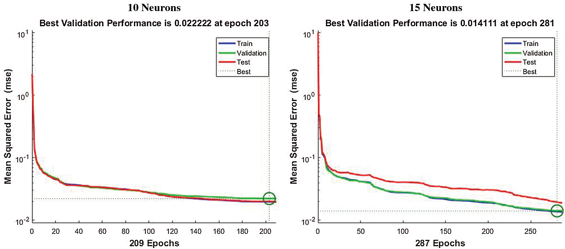
Figure 5: Performance of proposed system using scaled conjugate gradient algorithm with different number of neurons at hidden layer having emotion features
In other experiments, 15, 20, and 25 neurons were used in the hidden layer but no significant change in performance was observed after increasing the number of neurons from 15 at the hidden layer as shown in Fig. 5b. Fig. 6 gives the plot of regression using a similar network setting and the results were observed. It is observed that with 10 neurons at hidden layer though the network converged early the overall validation and testing accuracy remained at 89% (see Fig. 6a) and increasing the number of neurons after 15 the performance of the trained network with emotion features of the proposed system increased to approximately 91% (see Fig. 6b) but it is still low as compared to the training of LM algorithm. This indicates that changing the training algorithm implies no improvement of the performance and accuracy of the neural network and it may therefore be concluded that the LM algorithm for training neural network can give the best result for the training of the proposed system using 25 neurons at hidden layer.
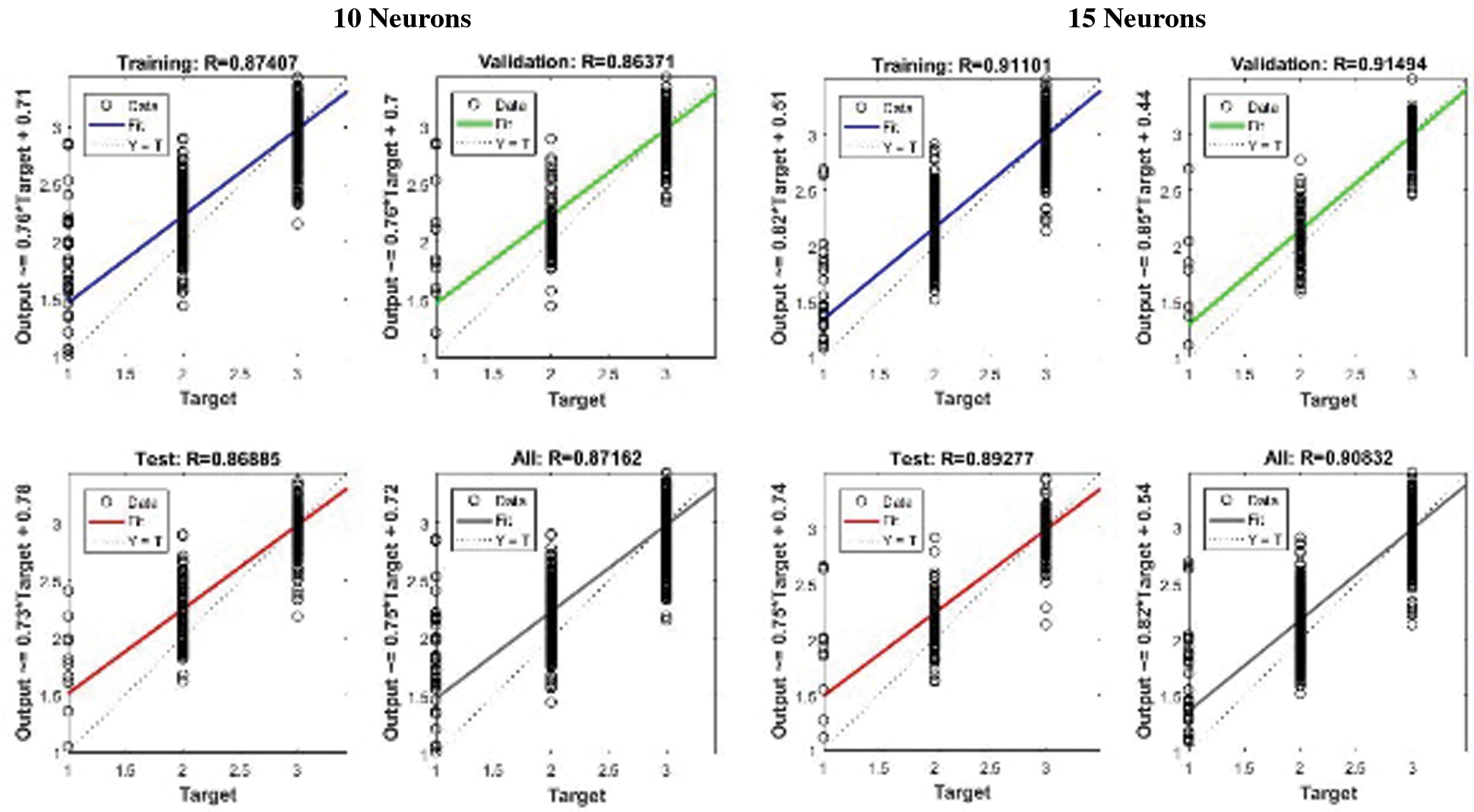
Figure 6: Comparison of regression for the proposed system using scaled conjugate gradient algorithm with different number of neurons at hidden layer having emotion features
It is hypothesized in this research in accordance with different theories of human psychology (see Section 2) that emotions play a significant role in the enhancement and depression of sensory stimuli. Therefore, it was necessary to conduct another set of experiments to test whether the behavior of the trained network is consistent with this hypothesis. Consequently, another set of experiments were conducted by training the LM algorithm with the same audio and visual stimuli without presenting the features extracted as emotions from visual and auditory stimuli.
The computational complexity of the proposed system is given in Fig. 7 which clearly shows that the computational complexity of the system increases with the increase in the number of neurons at the hidden layer but it is also observed that the increase in the number of neurons at hidden layer also increases the accuracy of neural network.
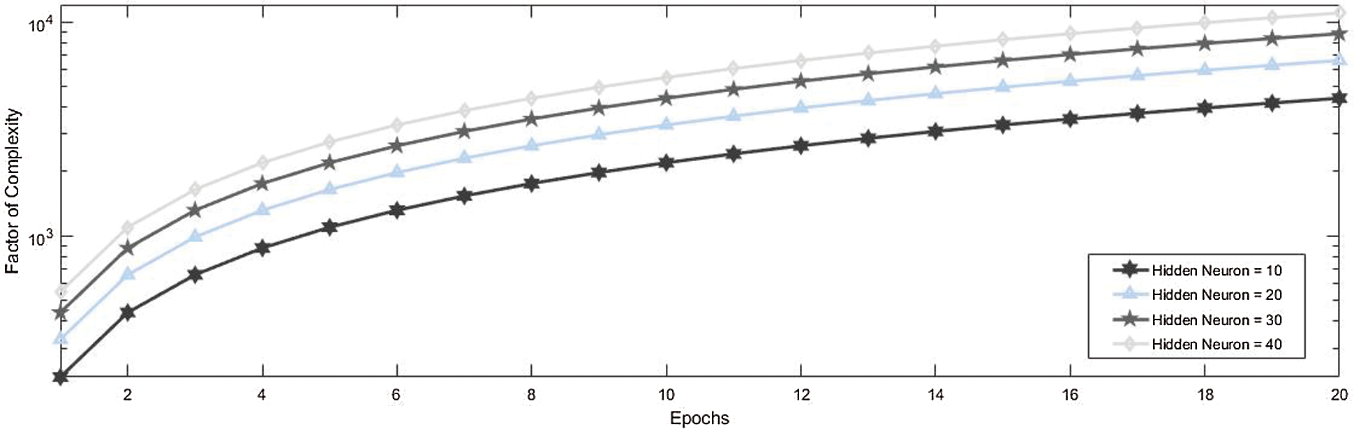
Figure 7: Factor of the complexity of neural network used in the proposed system with different numbers of neurons in a hidden layer
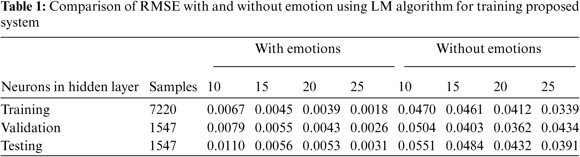
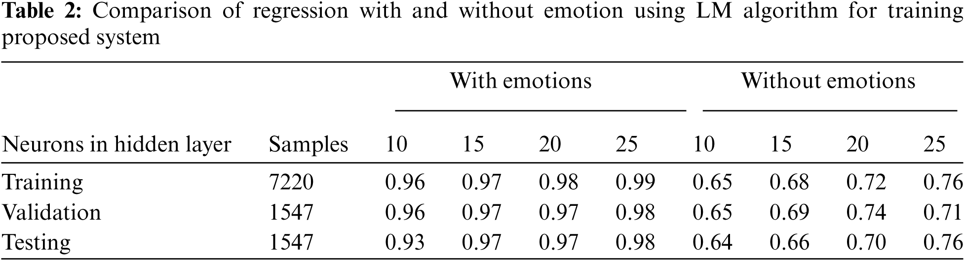
The comparison of Root means square error (RMSE) is given in Tab. 1 and the comparison of regression with or without the presence of emotion features. It is apparent from Tab. 1 and Tab. 2 that when emotion features are present in the dataset the RMSE decreases significantly as the number of neurons is increased up to a limit of 25 neurons in the hidden layer. Similarly, Tab. 2 shows that the accuracy of the system increases if emotion features are present during the training of the proposed system for signal enhancement and depression.
In this paper, various significant features of audio and visual signals and their impact on signal enhancement and depression are demonstrated. This paper proposes ANN-based system for signal enhancement and depression during the integration process of senses i.e., audio and visual. This paper presents a deeper insight into the modules of which this architecture is consisted of. This architecture provides the agent ability to localize the object based on enhancement and depression signals and find the effect of emotions on enhancement or depressed data employing audio and visual senses. It was observed that the enhancement and depression phenomena may take place in a large number of combinations of weak and strong stimuli. It is also observed that emotion plays a significant role in the enhancement and depression phenomenon and without the presence of emotions the accuracy of signal enhancement and depression decreases significantly.
Acknowledgement: Thanks to our families & colleagues who supported us morally.
Funding Statement: This work was supported by the GRRC program of Gyeonggi province. [GRRCGachon2020(B04), Development of AI-based Healthcare Devices].
Conflicts of Interest: The authors declare that they have no conflicts of interest to report regarding the present study.
1. R. Kiran, K. Michael, L. Jindong and W. Stefan, “Towards computational modelling of neural multimodal integration based on superior colliculus concept,” SN Applied Science, vol. 1, no. 1, pp. 269–291, 2013. [Google Scholar]
2. C. Laurent, L. Gerhard and W. Hermann, “Azimuthal sound localization using coincidence of timing across frequency on a robotic platform,” The Journal of the Acoustical Society of America, vol. 121, no. 4, pp. 2034–2048, 2007. [Google Scholar]
3. C. Cristiano, E. S. Barry and A. R. Benjamin, “Development of the mechanisms governing midbrain multisensory integration,” Journal of Neuroscience, vol. 38, no. 14, pp. 3453–3465, 2018. [Google Scholar]
4. F. Stan, M. Tamas, D. Sidney and S. Javier, “Lida: A systems-level architecture for cognition, emotion, and learning,” IEEE Transactions on Autonomous Mental Development, vol. 6, no. 1, pp. 19–41, 2014. [Google Scholar]
5. R. Sun, “The clarion cognitive architecture: Extending cognitive modeling to social simulation,” Cognition and Multi-Agent Interaction, vol. 10, no. 2, pp. 79–99, 2006. [Google Scholar]
6. D. Adele and C. Hans, “Bimodal and trimodal multisensory enhancement: Effects of stimulus onset and intensity on reaction time,” Perception & Psychophysics, vol. 66, no. 8, pp. 1388–1404, 2004. [Google Scholar]
7. A. Peiffer, J. Mozolic, C. Hugenschmidt and P. Laurienti, “Age-related multisensory enhancement in a simple audiovisual detection task,” Neuro Report, vol. 18, no. 10, pp. 1077–1081, 2007. [Google Scholar]
8. L. Lu, L. Fei, T. Feng, C. Yineng, D. Guozhong et al., “An exploratory study of multimodal interaction modeling based on neural computation,” Science China Information Sciences, vol. 59, no. 9, pp. 1–16, 2016. [Google Scholar]
9. Z. Zhang, G. Wen and S. Chen, “Multisensory data fusion technique and its application to welding process monitoring,” in IEEE Workshop on Advanced Robotics and its Social Impacts, IEEE Computer Society, Shanghai, China, pp. 20–24, 2016. [Google Scholar]
10. A. Balkenius and C. Balkenius, “Multimodal interaction in the insect brain,” BMC Neuroscience, vol. 17, no. 1, pp. 17–29, 2016. [Google Scholar]
11. H. H. Tseng, “Multisensory Emotional Recognition and Integration in the Ultra-High Risk State and Early Phase of Psychosis: An Fmri Study,” Kings College, London, pp. 1–55, 2013. [Google Scholar]
12. J. J. De, P. Hodiamont and G. B. De, “Modality-specific attention and multisensory integration of emotions in schizophrenia: Reduced regulatory effects,” Schizophrenia Research, vol. 122, no. 3, pp. 136–143, 2010. [Google Scholar]
13. B. Alicea, “Emergence and Complex Integration Processes: a neurophysiologically-inspired approach to information fusion in situation awareness,” in Department of Telecommunication, Information Studies, and Media and Cognitive Science Program, Michigan State University, Michigan, 2005. [Google Scholar]
14. Z. Mikhail, P. Carmen, C. Natalia, R. N. Andrey and M. Klaus, “Attention and multisensory integration of emotions in schizophrenia,” Front Hum Neuroscience, vol. 7, no. 1, pp. 674, 2013. [Google Scholar]
15. E. Thomas, P. Gilles and W. Dirk, “Investigating audiovisual integration of emotional signals in the human brain,” Progress in Brain Research, vol. 156, no. 1, pp. 345–361, 2006. [Google Scholar]
16. D. G. Beatrice, B. B. Koen, T. Jyrki, H. Menno and V. Jean, “The combined perception of emotion from voice and face: Early interaction revealed by human electric brain responses,” Neuroscience Letters, vol. 260, no. 1, pp. 133–136, 1999. [Google Scholar]
17. H. B. Andrew, M. Alex, V. O. John and P. M. Douglas, “Crossmodal integration in the primate superior colliculus underlying the preparation and initiation of saccadic eye movements,” Journal of Neurophysiology, vol. 93, no. 6, pp. 3659–3673, 2005. [Google Scholar]
18. U. Kniepert and P. R. Josef, “Auditory localization behaviour in visually deprived cats,” European Journal of Neuroscience, vol. 6, no. 1, pp. 149–160, 1994. [Google Scholar]
19. Y. Liping, C. Cristiano, X. Jinghong, A. R. Benjamin and E. S. Barry, “Cross-modal competition: The default computation for multisensory processing,” Journal of Neuroscience, vol. 39, no. 8, pp. 1374–1385, 2019. [Google Scholar]
20. M. Frens, O. A. Van and d. W. Van, “Spatial and temporal factors determine auditory-visual interactions in human saccadic eye movements,” Percept Psychophysics, vol. 57, no. 6, pp. 802–816, 2012. [Google Scholar]
21. U. Mauro, C. Cristiano and M. Elisa, “Sensory fusion: A neuro computational approach,” in Research and Technologies for Society and Industry Leveraging a Better Tomorrow, IEEE Computer Society, Bologna, Italy, pp. 1–5, 2016. [Google Scholar]
22. J. Middlebrooks and E. Knudsen, “A neural code for auditory space in the cat's superior colliculus,” The Journal of Neuroscience, vol. 4, no. 10, pp. 2621–2634, 2013. [Google Scholar]
23. P. Francesco, L. Elisabetta and D. Jon, “Auditory and multisensory aspects of visuospatial neglect,” TRENDS in Cognitive Sciences, vol. 7, no. 9, pp. 407–414, 2013. [Google Scholar]
24. K. H. Niclas, F. Elia and V. Jean, “Multisensory integration in speech processing: Neural mechanisms of cross-modal aftereffects,” Neural Mechanisms of Language, vol. 1, no. 3, pp. 105–127, 2017. [Google Scholar]
25. P. Neil, C. Chee-Ruiter, C. Scheier, D. Lewkowicz and S. Shimojo, “Development of multisensory spatial integration and perception in humans,” Development of Science, vol. 9, no. 5, pp. 454–464, 2016. [Google Scholar]
26. A. R, “Neural systems for recognizing emotion,” Current Opinion in Neurobiology, vol. 12, no. 2, pp. 169–177, 2012. [Google Scholar]
27. M. María and A. S. Miguel, “A new architecture for autonomous robots based on emotions,” International Journal of Social Robotics, vol. 3, no. 3, pp. 273–290, 2012. [Google Scholar]
28. F. R. Luis, R. Félix and W. Yingxu, “Cognitive computational models of emotions,” in 10th IEEE Int. Conf. on Cognitive Informatics and Cognitive Computing, USA, pp. 1–6, 2013. [Google Scholar]
29. E. S. Barry and R. S. Terrence, “Multisensory integration: current issues from the perspective of the single neuron,” Nature Reviews Neuroscience, vol. 9, no. 5, pp. 255–266, 2014. [Google Scholar]
30. H. M. Gurk and J. M. Donald, “Hearing lips and seeing voices,” Nature, vol. 264, no. 5588, pp. 746–748, 2014. [Google Scholar]
31. J. Wan, J. Huai and E. S. Barry, “Two corticotectal areas facilitate multisensory orientation behavior,” Journal of Cognitive Neuroscience, vol. 14, no. 8, pp. 1240–1255, 2012. [Google Scholar]
32. T. Brosch, K. Scherer, D. Grandjean and D. Sander, “The impact of emotion on perception, attention, memory, and decision-making,” Swiss Medical Weekly, vol. 5, no. 2, pp. 1–10, 2013. [Google Scholar]
33. M. White, “Representation of facial expressions of emotion,” the American Journal of Psychology, vol. 112, no. 3, pp. 371–381, 2012. [Google Scholar]
34. J. Wan and E. S. Barry, “Cortex controls multisensory depression in superior colliculus,” Journal of Neurophysiology, vol. 90, no. 4, pp. 2123–35, 2013. [Google Scholar]
35. C. Laurence, L. B. M. C. Viviane and P. Monique, “Compensating for age limits through emotional crossmodal integration,” Frontiers in Psychology, vol. 6, no. 1, pp. 691–704, 2015. [Google Scholar]
36. J. D. Raymond, D. G. Beatrice and J. Morris, “Crossmodal binding of fear in voice and face,” Proceedings of the National Academy of Sciences, vol. 98, no. 17, pp. 10006–10010, 2013. [Google Scholar]
37. K. R. Kiran, L. Jindong and B. Kevin, “Stimuli localization: An integration methodology inspired by the superior colliculus for audio and visual attention,” Procedia Computer Science, vol. 13, no. 1, pp. 31–42, 2012. [Google Scholar]
38. K. R. Kiran and B. Kevin, “A novel methodology for exploring enhancement and depression phenomena in multisensory localization: a biologically inspired solution from superior colliculus,” in Intelligent Systems and Signal Processing, Springer, Gujarat, India, vol. 1, no. 4, pp. 7–12, 2013. [Google Scholar]
39. E. S. Barry, R. S. Terrence and R. Benjamin, “Development of multisensory integration from the perspective of the individual neuron,” Nature Reviews Neuroscience, vol. 15, no. 1, pp. 520–535, 2014. [Google Scholar]
40. B. Johannes, D. C. Jorge and W. Stefan, “Modeling development of natural multi-sensory integration using neural self-organisation and probabilistic population codes,” Connection Science, vol. 27, no. 4, pp. 358–376, 2015. [Google Scholar]
41. J. M. Wei and P. Alexandre, “Linking neurons to behavior in multisensory perception: A computational review,” Brain Research, vol. 1242, no. 1, pp. 4–12, 2014. [Google Scholar]
42. L. S. Ashley, T. Marei and L. A. Brian, “Crossmodal plasticity in auditory, visual and multisensory cortical areas following noise-induced hearing loss in adulthood,” Hearing Research, vol. 343, no. 1, pp. 92–107, 2017. [Google Scholar]
43. S. Franklin, “Conscious software: A computational view of mind,” Soft Computing Agents: New Trends for Designing Autonomous Systems, vol. 75, no. 1, pp. 1–45, 2013. [Google Scholar]
44. L. Yuanqing, L. Jinyi, H. Biao, Y. Tianyou and S. Pei, “Crossmodal integration enhances neural representation of task-relevant features in audiovisual face perception,” Cerebral Cortex, vol. 25, no. 2, pp. 384–395, 2015. [Google Scholar]
45. M. A. Khan, S. Abbas, K. M. Khan, M. A. Ghamdi and A. Rehman, “Intelligent forecasting model of covid-19 novel coronavirus outbreak empowered with deep extreme learning machine,” Computers, Materials & Continua, vol. 64, no. 3, pp. 1329–1342, 2020. [Google Scholar]
46. A. H. Khan, M. A. Khan, S. Abbas, S. Y. Siddiqui, M. A. Saeed et al., “Simulation, modeling, and optimization of intelligent kidney disease predication empowered with computational intelligence approaches,” Computers, Materials & Continua, vol. 67, no. 2, pp. 1399–1412, 2021. [Google Scholar]
47. G. Ahmad, S. Alanazi, M. Alruwaili, F. Ahmad, M. A. Khan et al., “Intelligent ammunition detection and classification system using convolutional neural network,” Computers, Materials & Continua, vol. 67, no. 2, pp. 2585–2600, 2021. [Google Scholar]
48. B. Shoaib, Y. Javed, M. A. Khan, F. Ahmad, M. Majeed et al., “Prediction of time series empowered with a novel srekrls algorithm,” Computers, Materials & Continua, vol. 67, no. 2, pp. 1413–1427, 2021. [Google Scholar]
49. S. Aftab, S. Alanazi, M. Ahmad, M. A. Khan, A. Fatima et al., “Cloud-based diabetes decision support system using machine learning fusion,” Computers, Materials & Continua, vol. 68, no. 1, pp. 1341–1357, 2021. [Google Scholar]
50. Q. T. A. Khan, S. Abbas, M. A. Khan, A. Fatima, S. Alanazi et al., “Modelling intelligent driving behaviour using machine learning,” Computers, Materials & Continua, vol. 68, no. 3, pp. 3061–3077, 2021. [Google Scholar]
51. S. Hussain, R. A. Naqvi, S. Abbas, M. A. Khan, T. Sohail et al., “Trait based trustworthiness assessment in human-agent collaboration using multi-layer fuzzy inference approach,” IEEE Access, vol. 9, no. 4, pp. 73561–73574, 2021. [Google Scholar]
52. N. Tabassum, A. Ditta, T. Alyas, S. Abbas, H. Alquhayz et al., “Prediction of cloud ranking in a hyperconverged cloud ecosystem using machine learning,” Computers, Materials & Continua, vol. 67, no. 1, pp. 3129–3141, 2021. [Google Scholar]
53. M. W. Nadeem, H. G. Goh, M. A. Khan, M. Hussain, M. F. Mushtaq et al., “Fusion-based machine learning architecture for heart disease prediction,” Computers, Materials & Continua, vol. 67, no. 2, pp. 2481–2496, 2021. [Google Scholar]
54. A. I. Khan, S. A. R. Kazmi, A. Atta, M. F. Mushtaq, M. Idrees et al., “Intelligent cloud-based load balancing system empowered with fuzzy logic,” Computers, Materials and Continua, vol. 67, no. 1, pp. 519–528, 2021. [Google Scholar]
55. S. Y. Siddiqui, I. Naseer, M. A. Khan, M. F. Mushtaq, R. A. Naqvi et al., “Intelligent breast cancer prediction empowered with fusion and deep learning,” Computers, Materials and Continua, vol. 67, no. 1, pp. 1033–1049, 2021. [Google Scholar]
56. R. A. Naqvi, M. F. Mushtaq, N. A. Mian, M. A. Khan, M. A. Yousaf et al., “Coronavirus: A mild virus turned deadly infection,” Computers, Materials and Continua, vol. 67, no. 2, pp. 2631–2646, 2021. [Google Scholar]
57. A. Fatima, M. A. Khan, S. Abbas, M. Waqas, L. Anum et al., “Evaluation of planet factors of smart city through multi-layer fuzzy logic,” the Isc International Journal of Information Security, vol. 11, no. 3, pp. 51–58, 2019. [Google Scholar]
58. F. Alhaidari, S. H. Almotiri, M. A. A. Ghamdi, M. A. Khan, A. Rehman et al., “Intelligent software-defined network for cognitive routing optimization using deep extreme learning machine approach,” Computers, Materials and Continua, vol. 67, no. 1, pp. 1269–1285, 2021. [Google Scholar]
59. M. W. Nadeem, M. A. A. Ghamdi, M. Hussain, M. A. Khan, K. M. Khan et al., “Brain tumor analysis empowered with deep learning: A review, taxonomy, and future challenges,” Brain Sciences, vol. 10, no. 2, pp. 118–139, 2020. [Google Scholar]
60. A. Atta, S. Abbas, M. A. Khan, G. Ahmed and U. Farooq, “An adaptive approach: Smart traffic congestion control system,” Journal of King Saud University—Computer and Information Sciences, vol. 32, no. 9, pp. 1012–1019, 2020. [Google Scholar]
61. M. A. Khan, S. Abbas, A. Rehman, Y. Saeed, A. Zeb et al., “A machine learning approach for blockchain-based smart home networks security,” IEEE Network, vol. 35, no. 3, pp. 223–229, 2020. [Google Scholar]
62. M. A. Khan, M. Umair, M. A. Saleem, M. N. Ali and S. Abbas, “Cde using improved opposite-based swarm optimization for mimo systems,” Journal of Intelligent & Fuzzy Systems, vol. 37, no. 1, pp. 687–692, 2019. [Google Scholar]
63. M. A. Khan, M. Umair and M. A. Saleem, “Ga based adaptive receiver for mc-cdma system,” Turkish Journal of Electrical Engineering & Computer Sciences, vol. 23, no. 1, pp. 2267–2277, 2015. [Google Scholar]
 | This work is licensed under a Creative Commons Attribution 4.0 International License, which permits unrestricted use, distribution, and reproduction in any medium, provided the original work is properly cited. |