DOI:10.32604/cmc.2022.023254
| Computers, Materials & Continua DOI:10.32604/cmc.2022.023254 | |
| Article |
Rainfall Forecasting Using Machine Learning Algorithms for Localized Events
1Centre for Disaster Mitigation and Management, Vellore Institute of Technology, Vellore, 632014, India
2School of Computer Science and Engineering, Vellore Institute of Technology, Vellore, 632014, India
3Department of Computer Science and Information Engineering, National Yunlin University of Science and Technology, Yunlin, 64002, Taiwan
4Service Systems Technology Center, Industrial Technology Research Institute, Hsinchu, Taiwan
5School of Information Technology and Engineering, Vellore Institute of Technology, Vellore, 632014, India
6Geophysical Institute of Vladikavkaz Scientific Centre, Russian Academy of Sciences (RAS), Vladikavkaz, Russian Federation
*Corresponding Author: Chuan-Yu Chang. Email: chuanyu@yuntech.edu.tw
Received: 01 September 2021; Accepted: 16 December 2021
Abstract: A substantial amount of the Indian economy depends solely on agriculture. Rainfall, on the other hand, plays a significant role in agriculture–while an adequate amount of rainfall can be considered as a blessing, if the amount is inordinate or scant, it can ruin the entire hard work of the farmers. In this work, the rainfall dataset of the Vellore region, of Tamil Nadu, India, in the years 2021 and 2022 is forecasted using several machine learning algorithms. Feature engineering has been performed in this work in order to generate new features that remove all sorts of autocorrelation present in the data. On removal of autocorrelation, the data could be used for performing operations on the time-series data, which otherwise could only be performed on any other regular regression data. The work uses forecasting techniques like the AutoRegessive Integrated Moving Average (ARIMA) and exponential smoothening, and then the time-series data is further worked on using Long Short Term Memory (LSTM). Later, regression techniques are used by manipulating the dataset. The work is benchmarked with several evaluation metrics on a test dataset, where XGBoost Regression technique outperformed the test. The uniqueness of this work is that it forecasts the daily rainfall for the year 2021 and 2022 in Vellore region. This work can be extended in the future to predict rainfall over a bigger region based on previously recorded time-series data, which can help the farmers and common people to plan accordingly and take precautionary measures.
Keywords: Time-series; ARIMA; LSTM; regression; rainfall
Agriculture is one of the major pillars of the Indian economy, which stumps up $400 billion to the economy and involves a total of 58% of the Indian population [1]. Even during the global pandemic of COVID-19, the agricultural sector of India had played an extensive role in the Indian economy despite the humongous disorganization [2,3]. Several successful studies have proven the importance of rainfall behind agriculture. Numerous case studies highlight the impacts of rainfall in agriculture and the effects of climatic changes on rainfall that could affect agriculture in the future [4,5]. Similarly, crops also play an important role in affecting rainfall. The researchers have come up with several mathematical models drawing the parallelism between transpiration from the crops and rainfall [6–8]. The importance of rainfall is way beyond its contribution to agriculture–it helps in maintaining the ecological balance, and directly or indirectly benefits the entire ecosystem [9–11]. Investigative studies have shown that rainfall impacts the carbon exchange [12–14] of the ecosystem; it also has imputation for the community of animals and the overall dynamics [15,16] of the biodiversity.
In this work, analysis of time-series data has been carried out, using multiple machine learning approaches, for the rainfall dataset of the Vellore region of Tamil Nadu, India. The dataset comprises the complete rainfall data over a decade–a period of ten years, from 2010 to 2019–in the region. Furthermore, the work stars feature engineering, which has been carried out for improving the overall performance of the predictive modeling [17]. The outcome of feature engineering incorporates new features that further remove all sorts of autocorrelation present in the data. It concerns the overall transmutation of the assigned feature space with the purpose to diminish the error during modeling for the assigned objective. On dismissal of consolidated autocorrelation, the data could be used for executing procedures on the time-series data, which contrarily could only be achieved on any other conventional regression data. It is always challenging to pick the most appropriate methodology for dealing with the time-series data [18], as they may occupy precise attributes like a trend or a break.
The major contributions of this work are as follows:
• The proposed system forecasts the daily rainfall in Vellore region in the years 2021 and 2022 on a daily basis.
• This work uses forecasting methodologies like the AutoRegessive Integrated Moving Average (ARIMA) and the exponential smoothening for the short-term and very short-term forecasting of the data, as they are flexible and allow components that are ‘AutoRegressive’ or are ‘moving average’.
• Furthermore, the time-series data is operated on using Long Short Term Memory (LSTM) and the regression techniques are used by manipulating the dataset.
After trying out several models, this work compares the efficiency of them benchmarked with several accuracy metrics on a test dataset. The work considers a dataset of rainfall for a decade over a small region, however, in its prospect, it can be extended in the future to predict rainfall over a bigger region and multiple models could be combined for better accuracies and efficiencies.
Composite Vellore district lies between 12° 15’ to 13° 15’ North latitudes and 78° 20’ to79° 50’ East longitudes in Tamil Nadu State. It is bounded on the north by Chittoor District of Andhra Pradesh, on the South by Thiruvannamalai District, and the west by Krishnagiri District, and the East by Thiruvallur and Kanchipuram districts (Fig. 1). The geographical area of this district is 6077 sq. km. (5,92,018 Ha). Forest Department records show a total extent of 1,92,461 ha of land under forests in the Vellore district. Among this area, a total of 89% is reserved forest, 2.6% is reserved land and the remaining 8.4% is counted under unclassified forests. Vellore is the Head-Quarters of Vellore District–it is well connected by railways and bus routes to the major towns of the neighboring states like Andhra Pradesh, Karnataka, and Kerala as shown in Fig. 1.
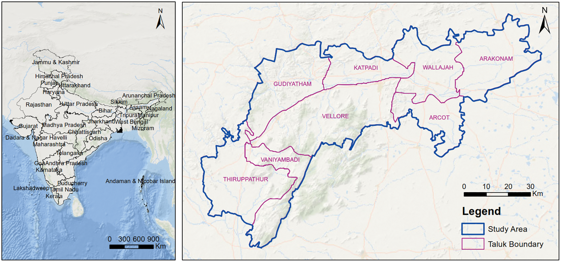
Figure 1: Location map of the study area and its administrative boundaries
Physiographically, the western parts of the district are endowed with hilly terrain and the eastern side of the district is mostly covered by rocky plains. The district has a population of 3,928,103 as per the 2011 census. The major rivers of the district are the Palar river and the Ponnai river. Generally, over a year, these rivers are almost always dry and sandy. The Palar river physically splits the district into 2 halves as it flows from Andhra Pradesh and enters the district at Vaniyambadi Taluk and passes through Ambur, Gudiyatham, Vellore, Katpadi, Wallajah, and Arcot Taluks. The Palar river had experienced floods at a frequency of once in 5 to 7 years–the last floods were reported in 1996 and 2001. The Ponnai river which flows from Andhra Pradesh enters the Vellore District at Katpadi Taluk and merges with the Palar river at Wallajah Taluk. Besides, Malattar, Koudinya Nadi, Goddar, Pambar, Agaram Aaru, Kallar, and Naganadi also flow through the district.
Generally, the temperature and rainfall in the district are moderate. The district records a maximum temperature of 40.2°C and a minimum of 19.5°C. Especially, Arakkonam Taluk enjoys a moderate climate throughout the year. On the other hand, Vellore, Walajah, and Gudiyatham Taluks–which are surrounded by hills–are subjected to extreme climate conditions either being very hot during summer or very cold during the winter season. In the Thirupathur Taluk, the climate is cold during winter but moderate during the other seasons. The district receives rainfall during the southwest and northeast monsoon period, and the average annual rainfall is around 976 mm. As per the study of the Tamil Nadu state Climate Change cell, Department of Environment, Government of Tamil Nadu, the annual rainfall for Vellore may reduce by 5.0% by the end of the century.
Though according to the simple probabilistic approach, the possibility of rainfall can be 50%–either it is going to rain, or it is not–in real life, however, several circumstances and other factors might turn the tables. It is possible to predict the occurrence of rainfall by studying the trends and exploring the patterns of previous rainfall over the region–in simple words, a place where it rains very often it would not be a surprise if it rains the other day, similarly, for a place where it has not rained over a significant period of time it can be predicted that it would not rain the other day. These are, however, predictions and can be proved, although very rare, to be inaccurate in some circumstances. In this work, various machine learning techniques are worked around on the rainfall dataset in order to compare and decide which method could be preferred over the others for precisely forecasting rainfall. The decision is based on several factors including their performance and accuracy scores. The architectural diagram of the proposed system is depicted by Fig. 2.
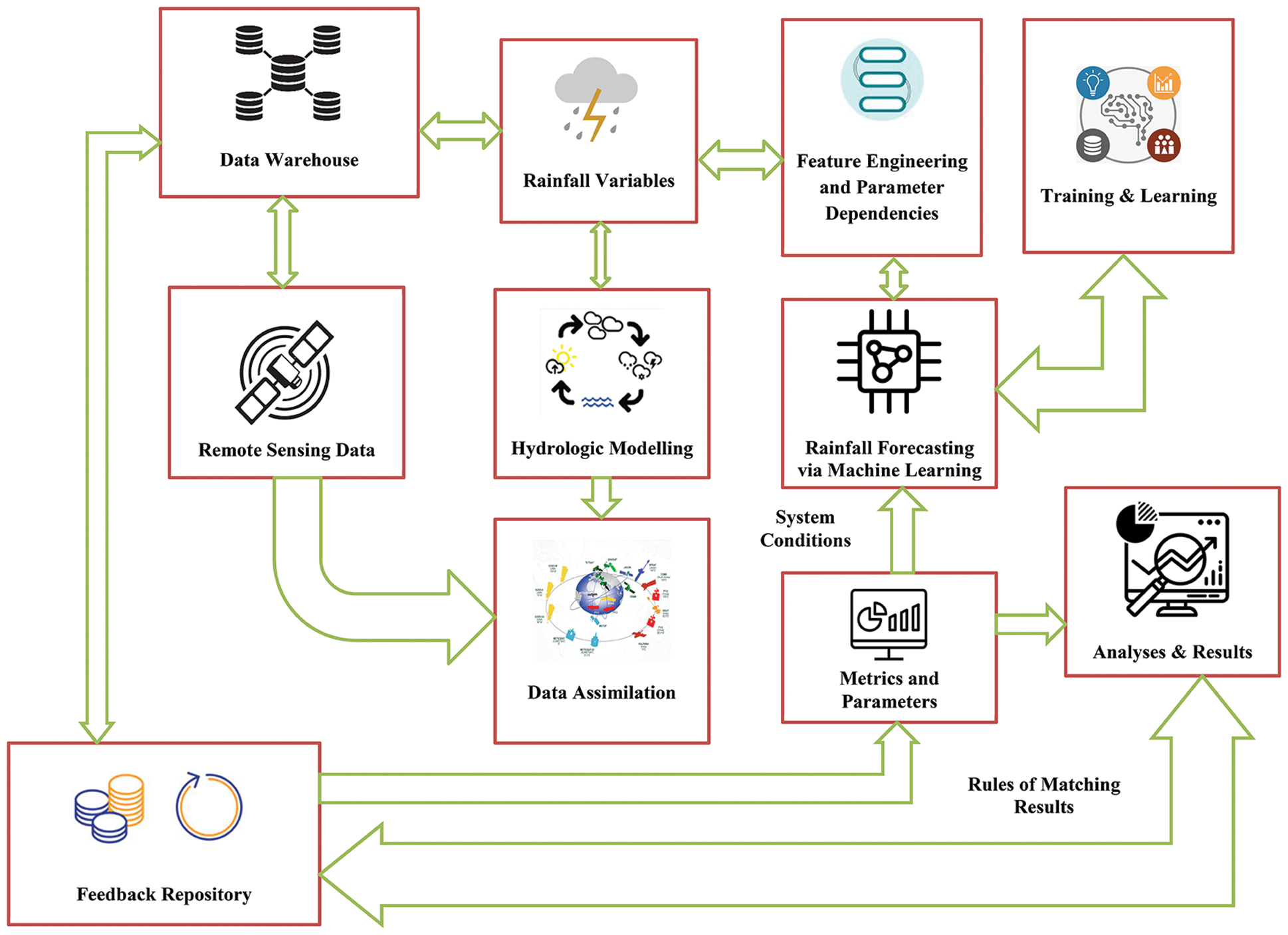
Figure 2: Architectural diagram of the proposed system
The raw rainfall data is collected from various meteorological departments as meteorological forcing variables, which later goes through hydrologic modeling for data assimilation. The data retrieved from the remote sensors of the satellites are also assimilated at that place. Further, the meteorological data and satellite data are stored in a data warehouse and further sent to the feedback repository. The feedback repository is used for rainfall data analysis by considering the metrics and the parameters. Since the metrics and the parameters are dynamic, the analysis updates from time to time. The analysis is also updated within the feedback repository. The meteorological data, in this work, is undergone feature engineering and parameters are extracted. Furthermore, the result is fed to the machine learning model for training and testing. After the training and testing are carried out on the dataset, the rainfall is finally forecasted.
The dataset is particularly time-series data comprising data of the annual rainfall in millimeters for ten years–from the year 2010 to the year 2019–around the Composite Vellore region of Tamil Nadu, India. It only consists of the dates and the rainfall measure in millimeters. The dataset has monthly distributions of rainfall over the places in Vellore–Alangayam, Ambur, Arakkonam, Arcot, Gudiyatham, Kaveripakkam, Melalathur, Sholingur, Tirupattur, Vaniyambad, Vellore, and Wallajah. To get a wholistic view to compare the rainfall in the study area, the total rainfall in the state of Tamil Nadu for the years 2010 to 2019 is presented in Fig. 3. The primary challenge of the dataset is present in the data itself–the climate of the Vellore region does not consist of a heavy rainfall pattern, in fact, even during the monsoon season it does not rain a lot. Hence, in order to test the different machine learning models for forecasting, the dataset is first cleaned by removing the empty details.
The machine learning models for forecasting consists of a wide range of techniques-from the conventional forecasting methodologies such as ARIMA [18,19] and Exponential smoothing to newer deep learning approaches such as LSTM [20]. It is no surprise that it can become very challenging to apply several regression techniques over time-series data–as the time-series data tend to have sparse values, so they shelter larger contributions to randomness than the seasonality of the data. For resolving the challenges of applying regression techniques on the time-series data [21], this work, furthermore, implements proper feature engineering. Long story short, the work acts as a rain predictor, which could help in predicting whether it is going to rain on a particular day or not in the Vellore region based on the dataset, and finally provide the quantity of rain in millimeters.
3.2.1 Preprocessing and Cleaning Data
The raw data might not be consistent all the time, they might contain empty values or incorrect values, and sometimes they even contain data that are irrelevant from an analysis perspective. These inconsistencies in the data could result in a disputed outcome that might include the failure of the entire model that is built [22]. As a result, the dataset needs to be reconsidered, after refining the data it contains-after removing unnecessary information, which could be overwhelming, and cleaning data by removing disparities. The dataset used in this work also has been cleaned by removing columns, which were not important from an analysis perspective, and replacing the values that were not a number or were irregular with zero.
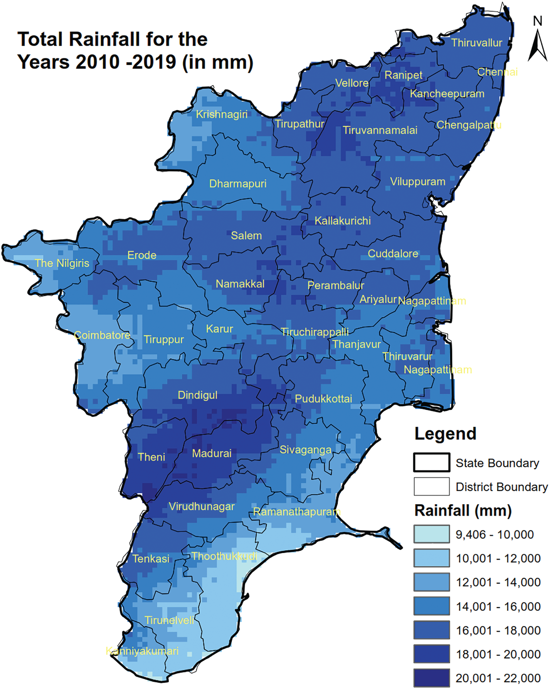
Figure 3: District wise total rainfall in the state of Tamil Nadu for the years 2010 to 2019
3.2.2 Exploratory Data Analysis
After the data has been refined, it was subjected to exploratory data analysis. The python library, Altair, has been used for having precise statistical visualization. The graphs helped in interpreting the trend of rainfall across different regions over the year for the entire decade [23]. The peaks and dips in the graphs helped in understanding the months when rainfall is higher and the months when it barely happens in the particular region.
3.2.3 Detecting Trend and Seasonality
In any time-series data, the component of the data that tends to alter over a period of time without repeating itself periodically is termed as its trend-it can be increasing or decreasing, linear or non-linear. In contrast to the trend of time-series data, seasonality can be defined as the component of the data that can modify over a span of time and also repeats itself. The trend and the seasonality are responsible for the time-series data to change at varying times. The dataset using in this work is statistically tested using Augmented Dickey-Fuller (ADF) test [24,25], where the null hypothesis is considered to be a unit root and the alternative hypothesis considers the time series to either be completely stationary or be stationary with respect to its trend. Furthermore, a lag in a time series data can be defined as the determined amount of time that has passed or has been delayed.
On performing the Augmented Dickey-Fuller Test on the refined dataset using lag equal to a period of a year, the test statistic value came out to be −2.24 and the critical value came out to be −2.56 for 10%. Since the test statistic value turned out to be slightly greater than the critical value, the null hypothesis of the ADF test is accepted and hence the alternative hypothesis is automatically rejected. So, the data used in this work is not stationary, but seasonal. The seasonality from the data is removed by differencing the data with an interval equal to that of the lag.
The Auto-Regressive Integrated Moving Average (ARIMA) model, at a high level, is an analysis model based on statistics. It is broadly used on time-series data, as it is known for providing better insight into the dataset and it also helps in predicting future trends [26]. While working with statistical models, the models that can predict the time-series data based on former data, it is called to be autoregressive. An autoregressive model can also seek to use a lag that could shift the entire time-series data–here, a lag of x means the model is capable of predicting the values by applying previous x terms of the dataset.
Further, another term that is frequently associated with the ARIMA model is moving average–which is another statistical measure used for the analysis of stock data. The moving average is widely used for analyzing time-series data–for the calculations of averages basing on a moving window [27]. There are three parameters associated with the ARIMA model, which need to be initialized beforehand–the autoregression lag, the differencing order for integration, and the moving average lag. For ARIMA model, the hyperparameters that are finally used include–an autoregression of 7 lags, and moving average of 1 lag.
3.2.5 Holt-Winters’ Exponential Smoothing Model
Another widely used model for forecasting time-series data is Holt Winters’ Exponential Smoothing–which manifests a trend in the dataset, as well as a seasonal variation [28]. The model has provisions of weighted averages–an average of x numbers, each of which is supplied a specific weight, and the denominator is determined by the sum of them–that help in forecasting based on the historical values where one could explicitly let the model know which values to put more emphasis on for the calculations.
The exponential smoothing methodology is able to forecast predictions using the weighted averages of all the previous values–In this case, the weights are made to sink exponentially from the data that is most recent to the one that is the oldest. It is considered by default that the latest data is much more important than older data [29]. Hence, it fails to acknowledge trends or seasonal variations in the time-series data. In contrast to this, Holt's exponential smoothing successfully acknowledges trends in time-series data but fails to consider seasonality. Finally, the Holt-Winters’ exponential smoothing solves the limitation and is able to consider both trend and seasonality. For Holt-Winter's Exponential Smoothing model, the hyperparameters that are finally used include seasonal periods value to be 12.
The Long Short Term Memory (LSTM) is a succession to the conventional Recurrent Neural Network and is extensively used for time-series data. In addition, it provides gates to keep the required information stored, and the layers that are fully connected provide a smooth flow of error across the gates. Each repeating module has several gates and several cell states, to apply functions onto the output from the previous cell and the input [30]. Furthermore, activation functions are added for filtering and modulating the data over the cells. LSTM is able to consider historical data to predict the forecast, and thus, is essentially used with time-series dataset having trends or seasonalities. In terms of the LSTM model, Bidirectional LSTM is used in this work. The hyperparameters include–4 blocks with 100 epochs, a ReLU (Rectified Liner Unit) activation layer, 1 dense output layer, and Adam optimizer for optimization. The loss is calculated using MAE (Mean Absolute Error) for identifying the model performance.
Regression cannot be applied to time-series data, as a result, the data needs to be converted to a regular dataset that cannot be autocorrelated. The rain dataset used in this work is time-series data that has trends and seasonality as analyzed from the previous investigation. However, the dataset is transformed into a regular dataset with the help of feature engineering-where new features are generated from the old features. The continuous data is converted into categorical ones, where for months and rainfall as shown in Tabs. 1 and 2. The months in Tab. 1 are mapped on the basis of notable seasonality in rainfall data–the value 2 shows the months of monsoon, and 1 shows the months of retreating monsoon in the Vellore region.
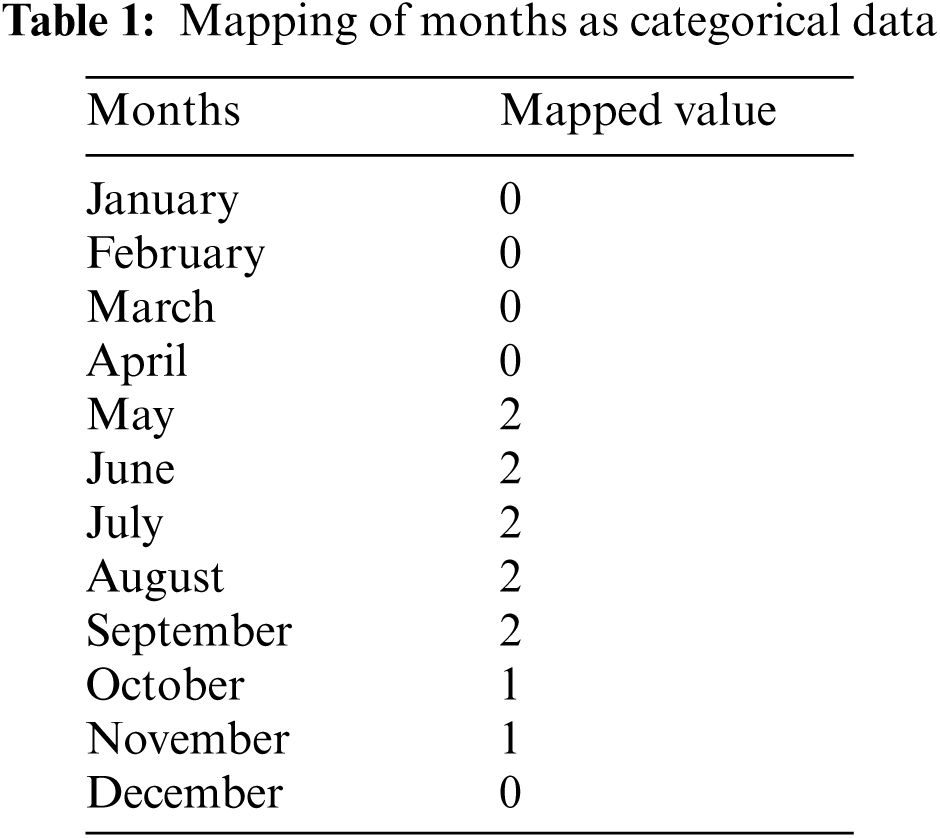
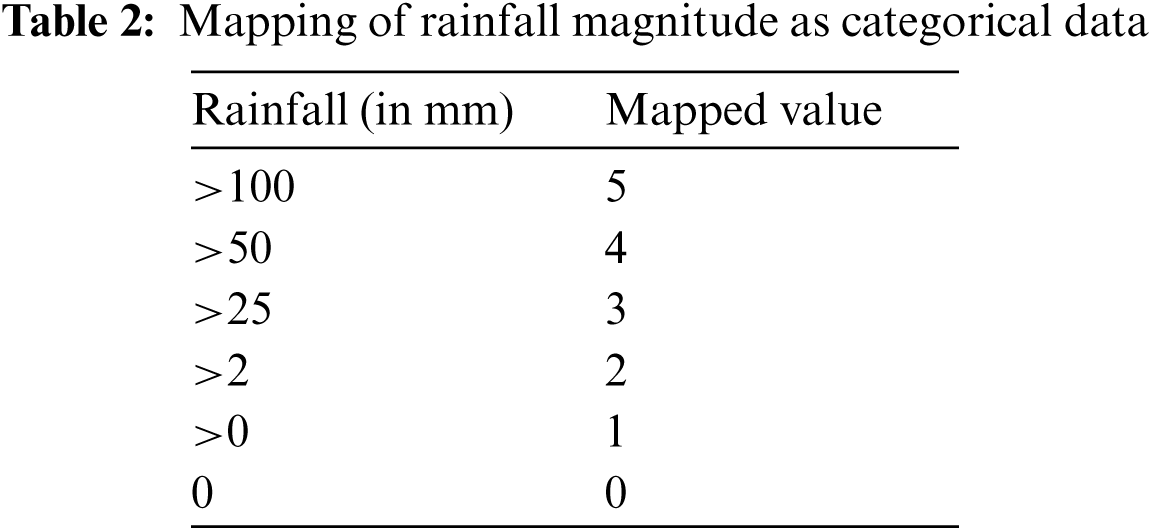
For Tab. 2, the rainfall data is mapped according to the frequency of magnitude –whenever it rains in the region, often, the magnitude is around 0–25 mm, while its rarely above 100 mm. Each of these new features is worked on different regression models for further analysis.
3.2.8 Support Vector Regression
Support Vector Regression (SVR) model is an advancement to the conventional Support Vector Machines (SVM)-which are widely used for solving the problems that are of classification categories [22]. The aim of SVR is to obtain a hyperplane-after boosting the dimensions of the dataset-and organize them into distinct classes. SVR employs a similar approach as that of SVM, except the fact that instead of assigning points into classes, the decision boundary lines and hyperplane, that are obtained, are used to search for the best fit line for the regression. For SVR model, Linear SVR is used as the hyperparameter where the regularization parameter is set to 0.1 and the epsilon-insensitive loss function is set to 5.
Linear Regression is another well-known regression model, which is very simple but still extensively used for classification problems. In this model, a linear equation is generated based on input and output variables, where the coefficients of the lines are generated during the learning process of the model [31]. After the formation of the linear equation, predictions can easily be obtained after solving the equation. Collinearity is usually removed from the data since a highly correlated input variable might adversely overfit the data.
XGBoost regression is an enhanced form of the conventional Gradient Boosting methodology. In gradient boosting, an ensemble algorithm is administered, where the umbrella term boosting encompasses the sequential addition of the models in the ensemble. Besides, the algorithm also governs multiple decision trees and assigns respective weights to these trees to explicitly give more importance to particular trees for determining the final output [32–35]. During the learning process of the model, the trainable parameters also learn through the gradient descent technique. The XGBoost in addition to the conventional Gradient Boosting algorithm reduces the overall time for training in a significant manner by optimizing the underlying hardware. This algorithm also has capabilities to handle sparse data–it, unlike Gradient Boosting, does not replace the zero values with the average values but chooses the best fit values while the learning process.
In this work, the XGBoost model is created using the hyperparameter values as–the base score is set to 0.5 that is the initial score of prediction of all instances, the booster is set as ‘gbtree’ that uses tree-based models. The step size shrinkage value of the model–which is also known as the learning rate, or the eta–is taken as 0.3 for preventing overfitting, and the minimum loss reduction value that is used in the model is used as 0 to make the algorithm less conservative. In addition to setting the importance type as gain, there are no other interaction and monotone constraints used, hence, the maximum delta step is set to be 0. The model does not use parallelization; thus, the number of parallel trees is set to 1.
The maximum depth of the tree is set as 35 with minimum summation of instance weight needed in the child set as 1–thus, every time partition occurs in the tree, the sum of instance weights of the nodes is less than 1. The L1 regularization is kept as 0, while the L2 regularization term on the weights is made to be 1. The seed, or what is also known as the random state is selected as 123. In addition, no verbosity is added to the model. Furthermore, the subsample ratios of the columns for each level, node and tree–while construction–is set to be 1, hence, while subsampling takes place, it occurs once when each tree is constructed, and once each new depth level is grasped in that tree and once during each period a new split is evaluated. Finally, a total of 3 estimators are used with exact greedy algorithm as the tree method–since the dataset is small.
The data from the dataset is visualized using different plots for better insight into it. The results of all the algorithms are compared using several different parameters, which are widely accepted. The final algorithm that is selected to be the best fit for the dataset is decided on the basis of these results. Before the analysis of the performances of each algorithm based on the score of their accuracy metrics, the dataset is individually envisioned. The plot of the autocorrelation of the magnitude of rainfall over a period of one year, along with lags from 0 to 365, is shown in Fig. 4.
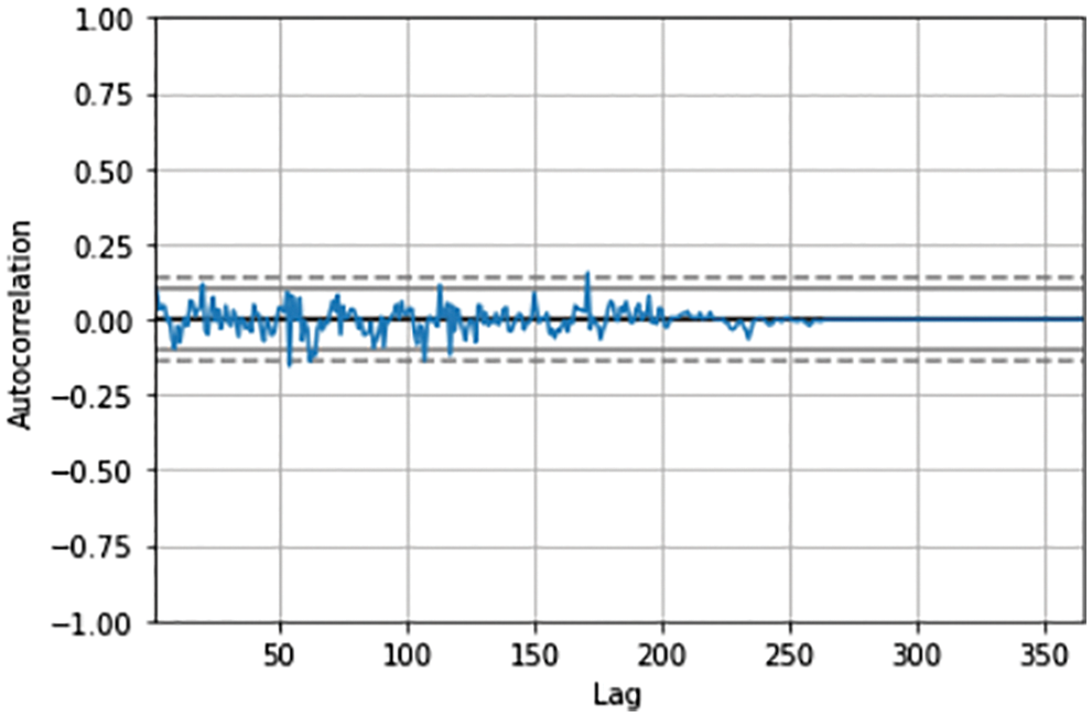
Figure 4: The autocorrelation plot of Alangayam Taluk during 2019 with lags from 0 to 365
It can be observed from Fig. 4, that the autocorrelation values approximately range between 0.125 and −0.125. This plot is of the Alangayam district of the Vellore region for the year 2019. The LSTM forecast plot of the Alangayam district during August 2019 can be seen in Fig. 5. It can be inferred that the prediction is not up to the mark for LSTM, as it fails to predict perfectly for most of the days. The disturbance in the curve can be seen in Fig. 5, when the lag is below 250, however, when the lag is above that, the autocorrelation is nearly 0. Regression cannot be implemented on dataset that are highly autocorrelated, hence feature engineering is carried out.
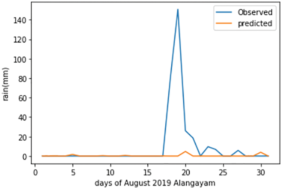
Figure 5: The LSTM forecast plot of Alangayam in Vellore district during August 2019
The SVR forecast plot of the Alangayam district during August 2019 can be seen in Fig. 6. It can be reasoned that the model cannot predict properly almost all of the days of August.
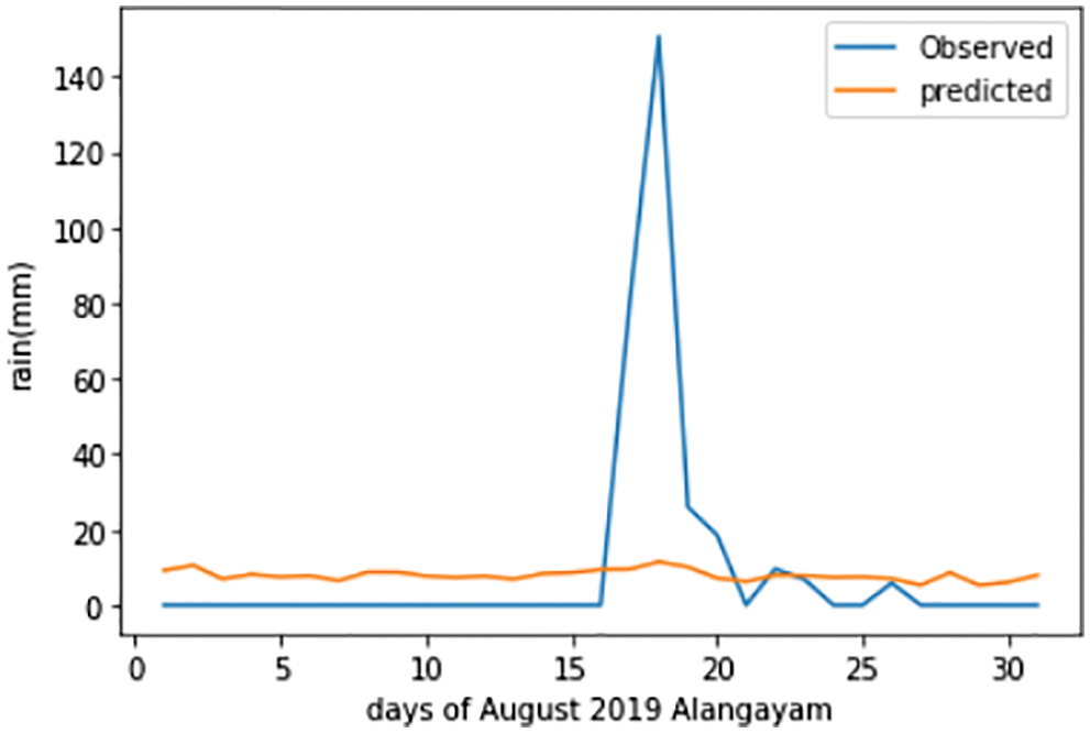
Figure 6: The SVR forecast plot of Alangayam in Vellore district during August 2019
The Linear Regression forecast plot of the Alangayam district during August 2019 can be seen in Fig. 7. It can be deduced that the prediction of the linear regression is worse than LSTM, however, it is better than the SVR.
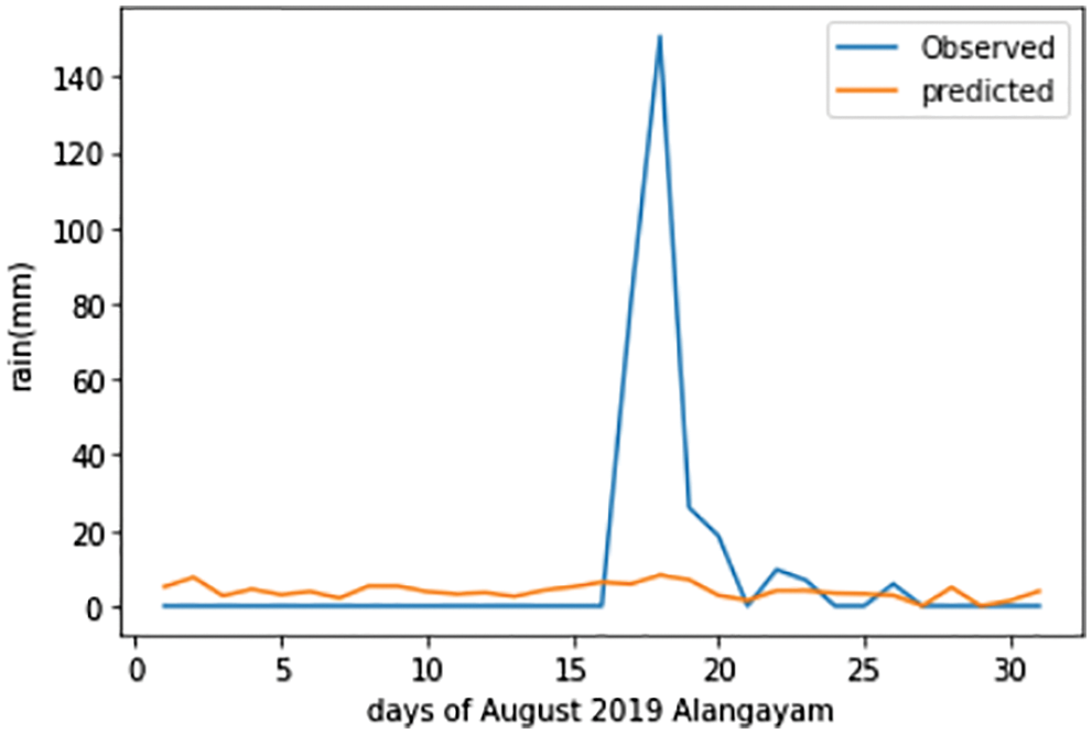
Figure 7: The linear regression forecast plot of Alangayam in Vellore district during August 2019
The XGBoost forecast plot of the Alangayam district during August 2019 can be seen in Fig. 8. It can be concluded that the model predicts with the most precision compared to the rest. However, the complete decision about the best-suited model for the dataset cannot simply be made of the prediction, but also the errors are needed to be taken into account.
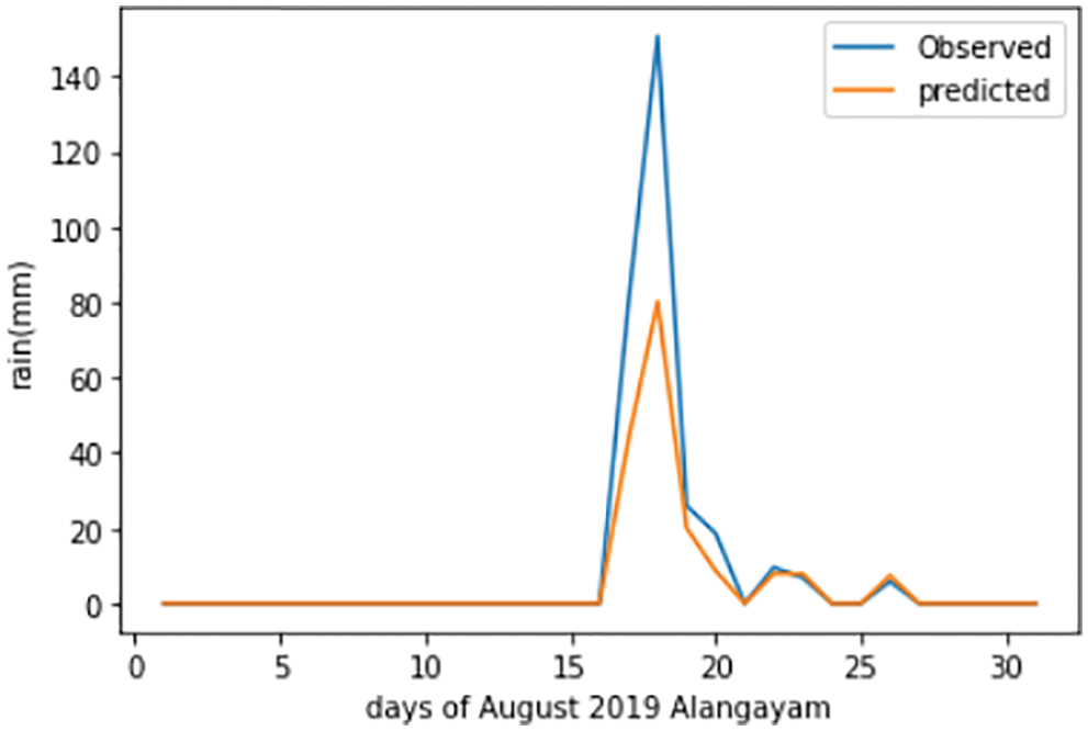
Figure 8: The XGBoost forecast plot of Alangayam in Vellore district during August 2019
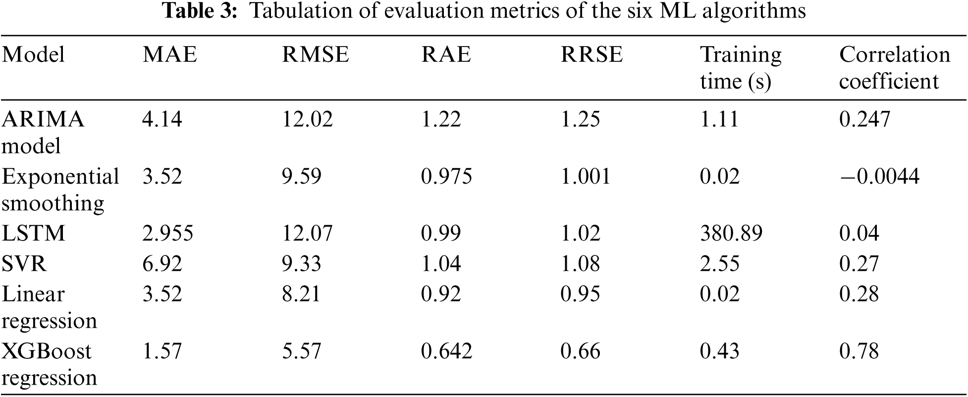
The Mean Absolute Error (MAE) is a widely used evaluation metric, where the average of the total absolute magnitude of errors is considered. The Root Mean Squared Error (RMSE) is another well-known evaluation metric that is calculated by taking the square root of the average of the sum of the squared error differences. Relative Absolute Error (RAE) is the total absolute error that further normalizes the final value by dividing it by the total absolute error of the simple predictor. Root Relative Squared Error (RRSE) takes the square root of the normalized squared error differences, where it is normalized by dividing with the total squared error of simple predictor.
The tabulation of the different evaluation metrics and magnitudes, for all six approaches, is shown in Tab. 3. From the table, it can be observed that the XGBoost Regression technique outnumbers all other techniques in terms of accuracy. It can further be observed that the time taken by LSTM is the most, which is nearly 6 min. From the correlation coefficient, it can be observed that exponential smoothing is not at all correlated, while XGBoost Regression is highly correlated.
The correlation coefficient and total training time plots of the six algorithms are shown in Figs. 9 and 10. It can be observed that in Exponential Smoothing has the least correlation while XGBoost has the highest correlation. The time taken for all the models except the LSTM model is very less, but that of the LSTM model is beyond 350 s.
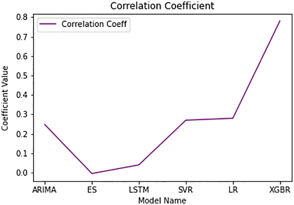
Figure 9: Comparative visualization of correlation coefficient of the models
To plot the data, the evaluation metrics are normalized for MAE, RMSE, RAE and RRSE. For normalizing the data, each column is divided with the maximum value of the respective column. The normalized values can be observed in Tab. 4.
The comparative visualization of the normalized MAE scores of the six algorithms are shown in Fig. 11. In the visualization, it can be observed that XGBoost has the least error score. With respect to MAE, the LSTM model has the second least error score followed by Linear Regression model.
The comparative visualization of the normalized RMSE scores of the six algorithms are shown in Fig. 12. In the plot, it can be observed that XGBoost has the least error score, just like MAE plot. In terms of RMSE, Linear Regression has second least error score followed by SVR.
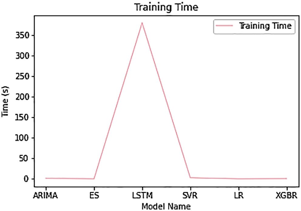
Figure 10: Comparative visualization of normalized RRSE score of the models
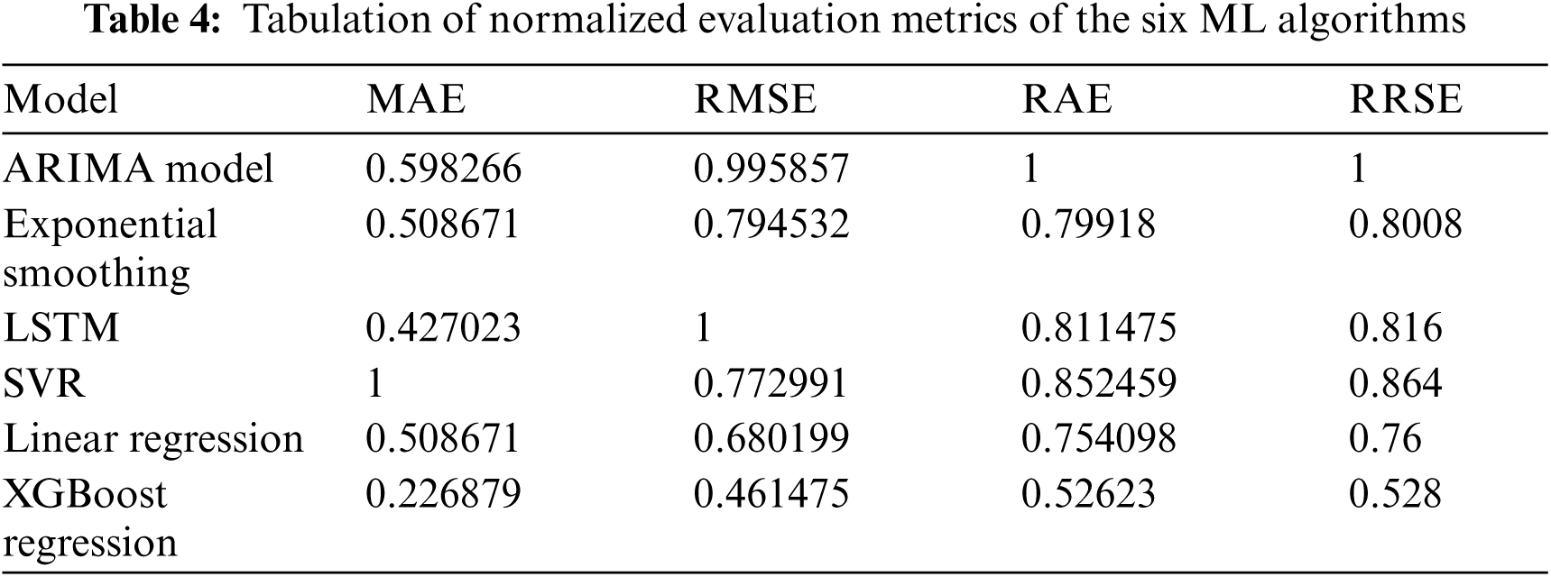
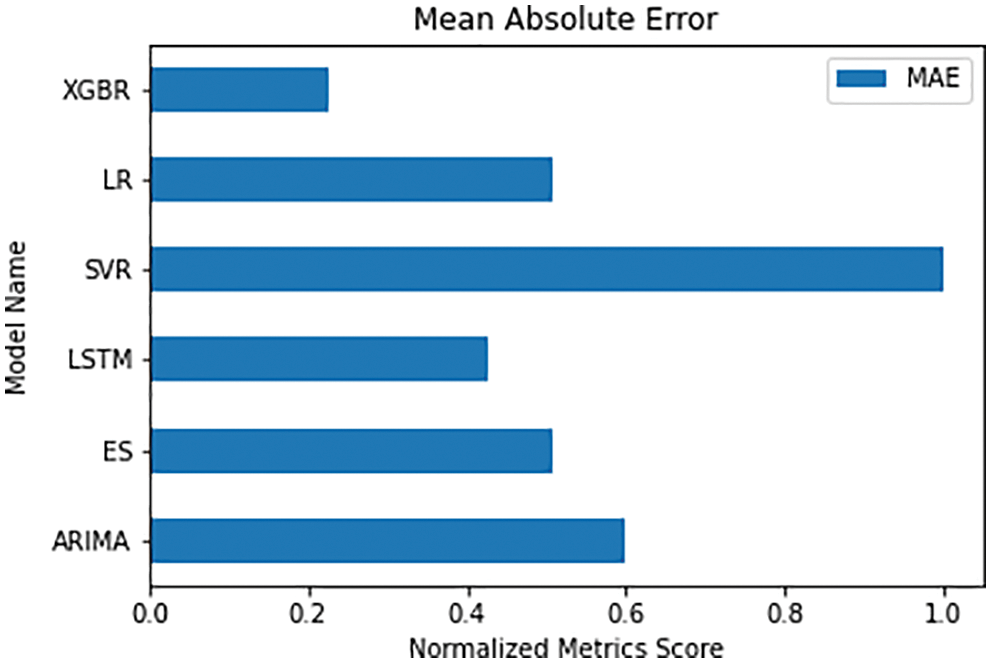
Figure 11: Comparative visualization of normalized MAE score of the models
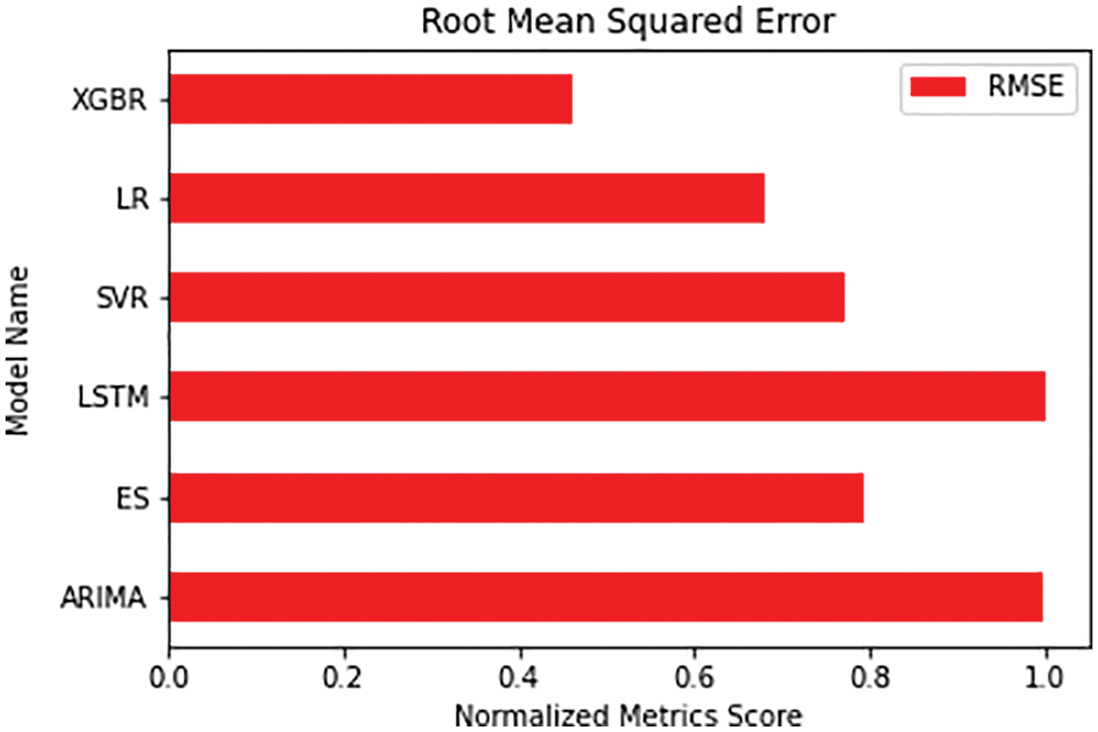
Figure 12: Comparative visualization of normalized RMSE score of the models
The normalized RAE metrics scores of the six algorithms are shown in Fig. 13. The plot shows that the XGBoost model has the least relative absolute error score. The Linear regression has second least score, followed by the Exponential Smoothing. The ARIMA model, on the other hand, has the most RAE score, followed by the SVR model and the LSTM model.
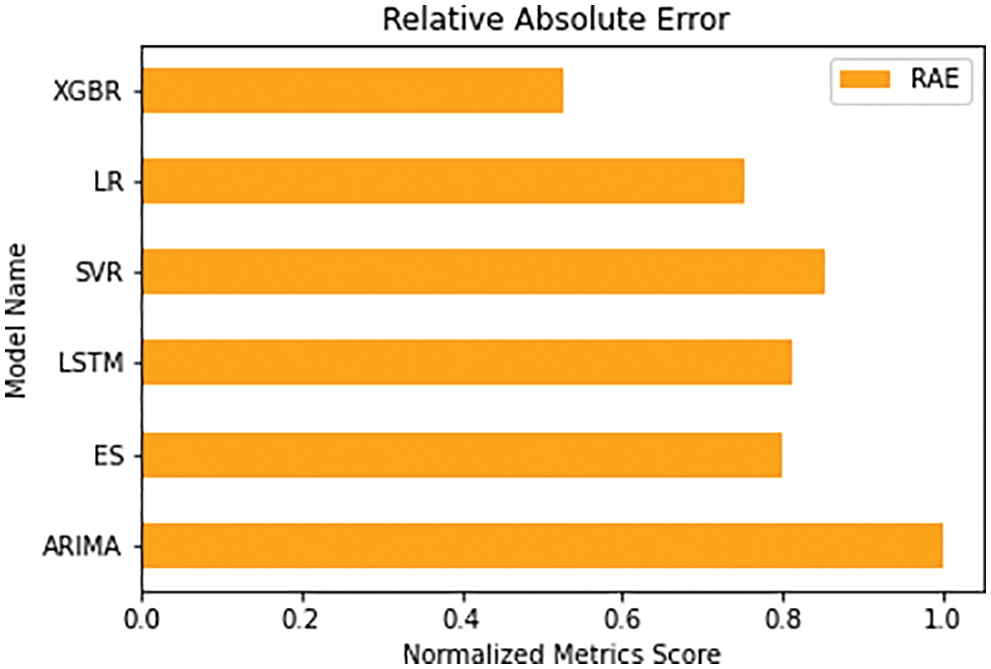
Figure 13: Comparative visualization of normalized RAE score of the models
The normalized RRSE metrics scores of the six algorithms are shown in Fig. 14. Both the scores–RAE and RRSE–follow similar trend and show that XGBoost has the least error score. Just like RAE plot, in RRSE plot too, the Linear regression has second least score, followed by the Exponential Smoothing.
Again, from all these visualization plots, it can be concluded that the XGBoost Regression technique surmounts the rest, and thus can be concluded as the best-suited algorithm for this dataset.
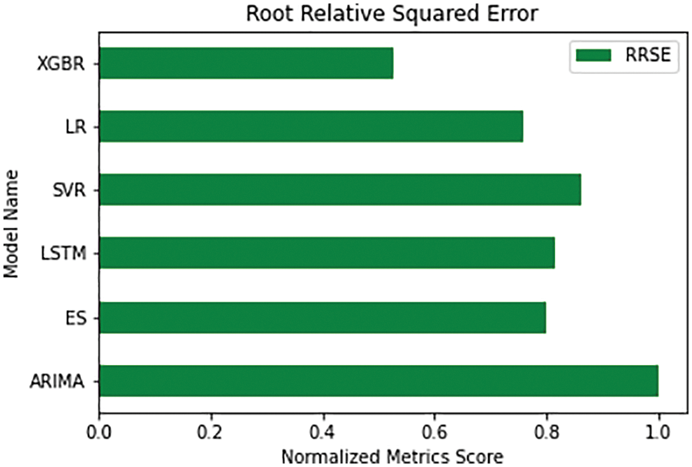
Figure 14: Comparative visualization of normalized RRSE score of the models
In this work, the rainfall dataset of the Vellore region is forecasted using six different algorithms–the ARIMA model, Holt-Winters’ Exponential Smoothing, LSTM, SVR, Linear Regression, and XGBoost Regression. However, since regression cannot be applied directly on time-series data, this work also discusses the feature engineering associated with converting the time-series data to regular data. After the models are successfully built, their predictions are individually assessed and plotted for better insight. Further, the accuracy metrics are evaluated based on–MAE, RMSE, RAE, and RRSE. The total time that is taken for training the models and the final correlation coefficient of the models are also considered for evaluation. After implementation, it was observed that the XGBoost Regression was able to predict most accurately compared to the rest. On the basis of the accuracy metrics plots, again it was observed that XGBoost Regression had the minimum overall error-based on MAE, RMSE, RAE, and RRSE. Another significant inferred point from the experimentation was that the LSTM took the highest amount of training time of six min. The correlation coefficient of XGBoost Regression was the highest and Holt-Winters’ Exponential Smoothing is not correlated. In the months of July to November, maximum rainfall is expected in Vellore region. Further, from February to April, months there would be minimum rainfall in Vellore region. Our proposed system forecasts the daily rainfall in Vellore region in the years 2021 and 2021 on a daily basis. Finally, it was concluded that the best-suited model for this dataset is XGBoost Regression. This work can be extended in the future for forecasting rainfall data using Deep Learning-which could be used for obtaining higher accuracy that would be beneficial for the meteorological department in predicting with better precision. Furthermore, the comparison can be widened by adding newer algorithms to the existing ones, or combining multiple algorithms for better results. Rainfall prediction could help people prepare themselves accordingly for disaster, and can help the agricultural sector on a broader scale.
Acknowledgement: Authors should thank those who contributed to the article but cannot include themselves.
Funding Statement: This research was partially funded by the “Intelligent Recognition Industry Service Research Center” from the Featured Areas Research Center Program within the framework of the Higher Education Sprout Project by the Ministry of Education (MOE) in Taiwan and Ministry of Science and Technology in Taiwan (Grant No. MOST 109-2221-E-224-048-MY2).
Conflicts of Interest: The authors declare that they have no conflicts of interest to report regarding the present study.
1. A. K. Singh, A. Upadhyaya, S. Kumari, P. K. Sundaram and P. Jeet, “Role of agriculture in making India $5 trillion economy under Corona pandemic circumstance: Role of agriculture in Indian economy,” Journal of AgriSearch, vol. 7, no. 2, pp. 54–58, 2020. [Google Scholar]
2. A. A. Cariappa, K. K. Acharya, C. A. Adhav, R. Sendhil and P. Ramasundaram, “Impact of COVID-19 on the Indian agricultural system: A 10-point strategy for post-pandemic recovery,” Outlook on Agriculture, vol. 50, no. 1, pp. 26–33, 2021. [Google Scholar]
3. C. Kyei-Mensah, R. Kyerematen and S. Adu-Acheampong, “Impact of rainfall variability on crop production within the Worobong ecological area of Fanteakwa district, Ghana,” Advances in Agriculture, vol. 2019, 2019. [Google Scholar]
4. D. Datta, D. Mittal, N. P. Mathew and J. Sairabanu, “Comparison of performance of parallel computation of CPU cores on CNN model,” in 2020 Int. Conf. on Emerging Trends in Information Technology and Engineering (ic-ETITEIEEE 2020, Vellore, India, pp. 1–8, 2020. [Google Scholar]
5. K. Srinivasan, L. Garg, D. Datta, A. A. Alaboudi, N. Jhanjhi et al., “Performance comparison of deep CNN models for detecting driver's distraction,” Computers, Materials & Continua, vol. 63, no. 3, pp. 4109–4124, 2021. [Google Scholar]
6. D. Datta and S. B. Jamalmohammed, “Image classification using CNN with multi-core and many-core architecture,” in Applications of Artificial Intelligence for Smart Technology, Pennsylvania, USA: IGI Global, 2021. [Google Scholar]
7. D. Elavarasan and P. M. D. R. Vincent, “Fuzzy deep learning-based crop yield prediction model for sustainable agronomical frameworks,” Neural Computing & Applications, vol. 33, pp. 13205–13224, 2021. [Google Scholar]
8. D. Datta, L. Garg, K. Srinivasan, A. Inoue, G. T. Reddy et al., “An efficient sound and data steganography based secure authentication system,” Computers, Materials & Continua, vol. 67, pp. 723–751, 2020. [Google Scholar]
9. D. Elavarasan and P. M. D. R. Vincent, “A reinforced random forest model for enhanced crop yield prediction by integrating agrarian parameters,” Journal of Ambient Intelligence and Humanized Computing, vol. 12, pp. 10009–10022, 2021. [Google Scholar]
10. D. Datta, P. K. Maurya, K. Srinivasan, C. Y. Chang, R. Agarwal et al., “Eye gaze detection based on computational visual perception and facial landmarks,” Computers, Materials & Continua, vol. 68, no. 2, pp. 2545–2561, 2021. [Google Scholar]
11. D. Elavarasan and D. R. Vincent, “Reinforced XGBoost machine learning model for sustainable intelligent agrarian applications,” Journal of Intelligent & Fuzzy Systems, vol. 39, no. 5, pp. 7605–7620, 2020. [Google Scholar]
12. D. Datta, P. E. David, D. Mittal and A. Jain, “Neural machine translation using recurrent neural network,” International Journal of Engineering and Advanced Technology, vol. 9, no. 4, pp. 1395–1400, 2020. [Google Scholar]
13. N. K. Arora, “Impact of climate change on agriculture production and its sustainable solutions,” Environmental Sustainability, vol. 2, pp. 95–96, 2019. [Google Scholar]
14. A. K. Misra and A. Tripathi, “Mathematical models of how the transpiration affects rainfall through agriculture crops,” Environmental Modeling & Assessment, vol. 26, pp. 837–848, 2021. [Google Scholar]
15. N. Singh, B. R. Parida, J. S. Charakborty and N. R. Patel, “Net ecosystem exchange of CO2 in deciduous Pine Forest of lower western Himalaya, India,” Resources, vol. 8, no. 2, pp. 98, 2019. [Google Scholar]
16. G. S. Bartzke, J. O. Ogutu, S. Mukhopadhyay, D. Mtui, H. T. Dublin et al., “Rainfall trends and variation in the Maasai Mara ecosystem and their implications for animal population and biodiversity dynamics,” PLoS One, vol. 13, no. 9, pp. 0202814, 2018. [Google Scholar]
17. J. Yan, T. Xu, Y. Yu and H. Xu, “Rainfall forecast model based on the TabNet model,” Water, vol. 13, no. 9, pp. 1272, 2021. [Google Scholar]
18. C. -C. Wang, C. -H. Chien and A. J. C. Trappey, “On the application of ARIMA and LSTM to predict order demand based on short lead time and on-time delivery requirements,” Processes, vol. 9, no. 7, pp. 1157, 2021. [Google Scholar]
19. R. Zhang, Z. Guo, Y. Meng, S. Wang, S. Li et al., “Comparison of ARIMA and LSTM in forecasting the incidence of HFMD combined and uncombined with exogenous meteorological variables in Ningbo, China,” International Journal of Environmental Research and Public Health, vol. 18, no. 11, pp. 6174, 2021. [Google Scholar]
20. P. S. Muhuri, P. Chatterjee, X. Yuan, K. Roy and A. Esterline, “Using a long short-term memory recurrent neural network (LSTM-RNN) to classify network attacks,” Information, vol. 11, no. 5, pp. 243, 2020. [Google Scholar]
21. G. Ciaburro and G. Iannace, “Machine learning-based algorithms to knowledge extraction from time series data: A review,” Data, vol. 6, no. 6, pp. 55, 2021. [Google Scholar]
22. C. Beyan, V. M. Katsageorgiou and R. B. Fisher “Extracting statistically significant behaviour from fish tracking data with and without large dataset cleaning,” IET Computer Vision, vol. 12, no. 2, pp. 162–170, 2018. [Google Scholar]
23. R. Roberts and R. Laramee, “Visualising business data: A survey,” Information, vol. 9, no. 11, pp. 285, 2018. [Google Scholar]
24. B. Li, J. Zhang, Y. He and Y. Wang, “Short-term load-forecasting method based on wavelet decomposition with second-order gray neural network model combined with ADF test,” IEEE Access, vol. 5, pp. 16324–16331, 2017. [Google Scholar]
25. E. Paparoditis and D. N. Politis, “The asymptotic size and power of the augmented Dickey–Fuller test for a unit root,” Econometric Reviews, vol. 37, no. 9, pp. 955–973, 2018. [Google Scholar]
26. M. Alsharif, M. Younes and J. Kim, “Time series ARIMA model for prediction of daily and monthly average global solar radiation: The case study of Seoul, South Korea,” Symmetry, vol. 11, no. 2, pp. 240, 2019. [Google Scholar]
27. E. Pacchin, S. Alvisi and M. Franchini, “A short-term water demand forecasting model using a moving window on previously observed data,” Water, vol. 9, no. 3, pp. 172, 2017. [Google Scholar]
28. S. Smyl, “A hybrid method of exponential smoothing and recurrent neural networks for time series forecasting,” International Journal of Forecasting, vol. 36, no. 1, pp. 75–85, 2020. [Google Scholar]
29. W. Jiang, X. Wu, Y. Gong, W. Yu and X. Zhong, “Holt–Winters smoothing enhanced by fruit fly optimization algorithm to forecast monthly electricity consumption,” Energy, vol. 193, pp. 116779, 2020. [Google Scholar]
30. F. Karim, S. Majumdar, H. Darabi and S. Chen, “LSTM fully convolutional networks for time series classification,” IEEE Access, vol. 6, pp. 1662–1669, 2018. [Google Scholar]
31. A. Al-Fugara, A. N. Mabdeh, M. Ahmadlou, H. R. Pourghasemi, R. Al-Adamat et al., “Wildland fire susceptibility mapping using support vector regression and adaptive neuro-fuzzy inference system-based whale optimization algorithm and simulated annealing,” ISPRS International Journal of Geo-Information, vol. 10, no. 6, pp. 382, 2021. [Google Scholar]
32. S. W. Kim, D. Jung and Y. -J. Choung, “Development of a multiple linear regression model for meteorological drought index estimation based on landsat satellite imagery,” Water, vol. 12, no. 12, pp. 3393, 2020. [Google Scholar]
33. S. I. Majid, S. W. Shah and S. N. K. Marwat, “Applications of extreme gradient boosting for intelligent handovers from 4G to 5G (mm waves) technology with partial radio contact,” Electronics, vol. 9, no. 4, pp. 545, 2020. [Google Scholar]
34. J. Alzubi, A. Nayyar and A. Kumar, “Machine learning from theory to algorithm: An overview,” in Journal of Physics: Conf Series, IOP Publishing, vol. 1142, no. 1, pp. 012012, 2018. [Google Scholar]
35. A. Jain and A. Nayyar, “Machine learning and its applicability in networking,” in New Age Analytics, New Jersey, USA: Apple Academic Press, pp. 57–79, 2020. [Google Scholar]
 | This work is licensed under a Creative Commons Attribution 4.0 International License, which permits unrestricted use, distribution, and reproduction in any medium, provided the original work is properly cited. |