Computers, Materials & Continua DOI:10.32604/cmc.2022.022328
Article

Gauss Gradient and SURF Features for Landmine Detection from GPR Images

Fatma M. El-Ghamry1,2, Walid El-Shafai2, Mahmouad I. Abdalla1, Ghada M. El-Banby3, Abeer D. Algarni4,*, Moawad I. Dessouky2, Adel S. Elfishawy2, Fathi E. Abd El-Samie2,4 and Naglaa F. Soliman1,4

1Department of Electronics and Communications Engineering, Faculty of Engineering, Zagazig University, Zagazig, Sharqia, 44519, Egypt
2Department of Electronics and Electrical Communications Engineering, Faculty of Electronic Engineering, Menoufia University, Menoufia, 32952, Egypt
3Department of Industrial Electronics and Control Engineering, Faculty of Electronic Engineering, Menoufia University, Menouf, 32952, Egypt
4Department of Information Technology, College of Computer and Information Sciences, Princess Nourah Bint Abdulrahman University, Riyadh, Saudi Arabia
*Corresponding Author: Abeer D. Algarni. Email: adalqarni@pnu.edu.sa
Received: 04 August 2021; Accepted: 15 September 2021

Abstract: Recently, ground-penetrating radar (GPR) has been extended as a well-known area to investigate the subsurface objects. However, its output has a low resolution, and it needs more processing for more interpretation. This paper presents two algorithms for landmine detection from GPR images. The first algorithm depends on a multi-scale technique. A Gaussian kernel with a particular scale is convolved with the image, and after that, two gradients are estimated; horizontal and vertical gradients. Then, histogram and cumulative histogram are estimated for the overall gradient image. The bin values on the cumulative histogram are used for discrimination between images with and without landmines. Moreover, a neural classifier is used to classify images with cumulative histograms as feature vectors. The second algorithm is based on scale-space analysis with the number of speeded-up robust feature (SURF) points as the key parameter for classification. In addition, this paper presents a framework for size reduction of GPR images based on decimation for efficient storage. The further classification steps can be performed on images after interpolation. The sensitivity of classification accuracy to the interpolation process is studied in detail.

Keywords: GPR images; cumulative histogram; gradient image; neural classifier; SURF

1  Introduction

Landmines are explosive objects buried at certain depths underground. Landmine detection is very vital for the efforts of re-cultivation and civilization. Different types of landmines have been implanted during wars in different areas of the world. Detection of landmines can be performed with different techniques such as electromagnetic, acoustic, optical, mechanical, biological, and nuclear techniques [1–4]. The GPR is one of the most efficient landmine detection techniques. Khan et al. [5] developed a landmine detection technique from GPR scans based on assuming that GPR images can be interpreted in a 1-D format. GPR images resemble speech signals in nature. The authors developed a landmine detection technique based on extracting cepstral features from the GPR images and using neural classification. Although this technique is simple, it destroys the 2-D nature of images and the 2-D geometry of objects.

Hamdi and Figui [6] presented a GPR landmine detection technique based on an ensemble hidden Markov model. They proved that the different textures of landmine activities are reflected in their model parameters. Furthermore, they compared their technique with a baseline HMM and demonstrated the superiority of their technique to this model. This technique achieved up to 95% detection accuracy.

Klesk et al. [7] presented landmine detection approach from 3-D scans taken at different levels underground using higher-order statistics. This approach firstly generates integral images, and hence higher-order moments are extracted from these integral images in a constant time. This approach achieved different sensitivity values up to 98% and different false alarm values down to 2% with different types of landmines.

There are several problems facing the use of GPR as a real-time detector for underground utilities. The background noise is one of these problems. It seems as large-amplitude, low-frequency, horizontal stripes in GPR images. Ali and Hussein [8] proposed a proficient background removal algorithm that can be incorporated into GPR logging devices.

Several resources in the world are not utilized due to landmines. Deep analysis and several test cases can be studied to guarantee a reliable landmine sensing system. 2D finite element models have been proposed for different objects in the sand at different depths in [9]. This inverse approach is based on neural networks. It is considered a reliable and proficient tool for landmine detection to accurately estimate the basic parameters of the landmine (type, depth) in a sandy desert.

Data processing includes extracting important information from any dataset. It is basically different from data analysis because it includes an algorithm that changes the original data, while the analysis encompasses temporary operations preliminary to processing steps or useful to achieve improved data component visualization and discrimination. Several algorithms that can be applied to GPR data can be used in other fields such as image processing [10]. In addition, the authors of [11] proposed an innovative fully non-linear multi-frequency multi-scaling approach for processing of wide-band GPR measurements.

The rest of this paper is organized as follows. In Section 2, the related work is presented. The two proposed algorithms are introduced in Section 3. In Section 4, the efficient storage of landmine images is discussed. The simulation results are presented in Section 5. Finally, Section 6 gives the conclusions.

2  Related Work

2.1 GPR Technique

The state-of-the-art GPR system is used for identifying subsurface irregularities. This tool has proven to be of high proficiency and practicality. The GPR is one of the most widely-used electromagnetic techniques for landmine detection due to its advantages compared to other tools, as it is simple and can be easily used. It consumes low power. It can find mines with any type of casing, and it can detect plastic objects. Hence, the GPR can be used in a wide range of applications such as engineering, archaeology, and geological applications [12].

The first stage for any GPR detection technique is the sensor. GPR can be developed in software and hardware. This research concentrates on GPR software techniques. Simply, the core of GPR work is that it consists of two antennas, as illustrated in Fig. 1. The transmitter antenna sends a signal into the subsurface that needs to be detected in the form of an electromagnetic wave. When this wave or signal reaches the ground, it will be reflected. Refraction and diffraction from materials occur, when there is a difference in the dielectric properties. After that, the receiver antenna receives the reflected signal, and then this signal can be processed to determine what it identified depending on the results of the processing method [7].

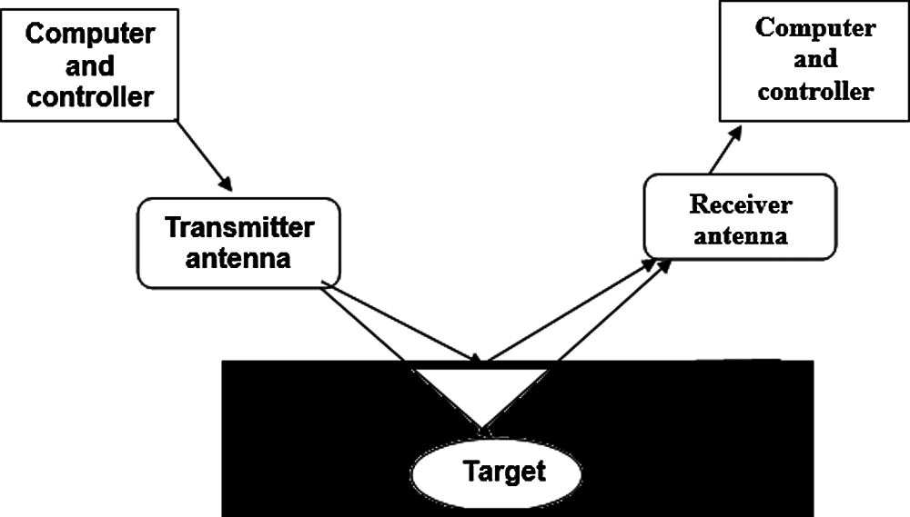
Figure 1: Basic GPR system

The GPR usually uses a frequency band ranging from 100 to 100 GHz. Processing of the results can lead to more information, such as the depth of buried objects. The depth can be known by computing the time consumed to receive the signal that is transmitted and then reflected. The sub-surface features can also be obtained for the buried objects, which may be landmines, rocks, metals, underground water, or gold. By translating the reflected electromagnetic wave and studying the dielectric properties, we can easily understand what it refers to. This can be done by determining the properties such as permittivity, magnetic susceptibility, and conductivity of the media [13].

The depth that the GPR wave can penetrate depends on the humidity of the earth and the wavelength of the wave. There are some limits for that depth, like the electrical conductivity of the ground, the center frequency of the transmitter antenna, and the radiated power.

On the other hand, when the electrical conductivity increases, attenuation in the electromagnetic wave is increased. The GPR cannot investigate more depth with higher frequencies, but the resolution may be improved. Therefore, the choice of frequency depends on the type of application. The application should make a balance between resolution and depth. In addition, the GPR is used in several applications like studying bedrocks, soil types, roads, mapping of archaeological features, and landmine detection [14].

2.2 Microwave Radiometry (MWR)

This technique is based on transmitting short radio and microwave (102 to 3 × 103 MHz) radiation pulses from an antenna into the ground and measuring the time for reflections to return to the same antenna. Reflections occur at the boundaries between materials of different dielectric constants that are normal to the incident radiation [15]. Transmission of high frequencies provides a high resolution, but with high attenuation in the soil. Hence, high frequencies are suitable for the detection of small shallow objects. Conversely, low frequencies achieve a lower resolution, but are less attenuated in the soil. Hence, low frequencies are more suitable for detecting deep objects. The MWR technique can give good results in dry soils, but it does not achieve good results in wet soils [16].

2.3 Infrared (IR) Detection

The IR radiation is a portion of the electromagnetic radiation spectrum between the visible light and microwave with wavelengths between 0.75 μm and 1 mm. The concept of using IR thermography for mine detection is based on the fact that mines might have different thermal properties from the surrounding materials. The IR sensor is safe with light weight, and it can scan large areas. However, IR sensors have difficulty in detecting deep objects [17].

3  Proposed Techniques for Landmine Detection

This section presents two proposed landmine detection techniques. These techniques are based on the Gauss gradient and the SURF descriptor.

3.1 Landmine Detection Based on Cumulative Histogram of Gradients

As shown in Fig. 2, a histogram-based strategy is adopted for landmine detection. The basic idea of this strategy is to apply a Gaussian kernel on the image with a certain scale. After that, a Laplacian gradient is used to generate an edge map for the image at the selected scale. The histogram is obtained for this edge map. The histogram of the edges is not enough to decide whether a landmine exists or not. So, a cumulative histogram is generated for each case. After carefully considering the cumulative histograms for the cases with and without landmines, we can select specific gray levels for discrimination based on the cumulative histogram values at these levels in the presence and absence of landmines.

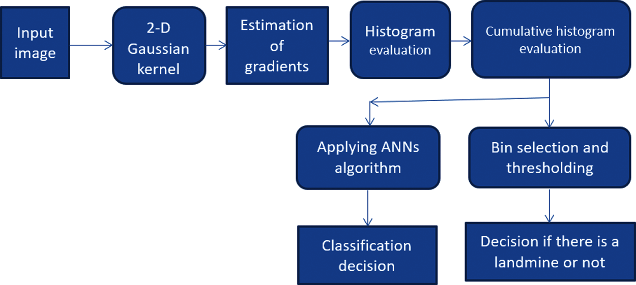
Figure 2: Block diagram of the proposed algorithm

Consider a gray-scale image as a function f(x, y). The following Gaussian kernel is applied on the image [18]:

G(x,y)=12πσ2e−(x2+y2)2σ2(1)

Instead of estimating the Laplacian of the image after applying the Gaussian kernel, an alternative approach is to directly apply the Gaussian kernel derivatives in both x and y directions on the image. The derivative of the Gauss kernel in Eq. (1) with x is given by [18]:

Gdx=∂G(x,y)∂x=−xG(x,y)σ2(2)

Also, the derivative with y is given by [18]:

Gdy=∂G(x,y)∂y=−xG(x,y)σ2(3)

Due to the commutative property between the derivative operator and the Gaussian smoothing operator, such scale-space derivatives can equivalently be computed by convolving the original imagef(x,y) with the Gaussian derivative operators [Gdx,Gdy]. This means that the edge map components in both x and y directions are given by [19],

Dfx=Gdx⊗f(x,y)(4)

Dfy=Gdy⊗f(x,y)(5)

From Eqs. (4) and (5), we deduce that both DfxandDfy reveal the image details due to the derivative effect, where ⊗ refers to the convolution operation [20]. The proposed approach depends on estimating the details in a common image format as follows [19]:

Dfxy=|Dfx|+|Dfy|(6)

Finally, from Eq. (6), we can work on the histogram ofDfxy.

Gauss gradient algorithm has been applied on more than 70 images with and without landmines. Both the histogram and cumulative histogram have been estimated for all images. Always, there is a difference between the cumulative histogram curves of both types of images. So, a threshold can be set in the middle of the two curves at a particular bin value. Thus, it is possible to discriminate between two images with and without landmines by setting a threshold at a certain bin value in the cumulative histogram. Therefore, we can adopt this strategy for discrimination by taking the bin level of 50, for example, and setting a threshold equal to 0.6. Moreover, we can also use neural classification in this task.

3.2 SURF-Based Landmine Detection

The proposed algorithm for landmine detection based on SURF features includes extracting the SUFR points of the images containing landmines and the images without landmines. Then, based on the volume of the feature vector, a decision is taken whether a landmine exists or not, as shown in Fig. 3.

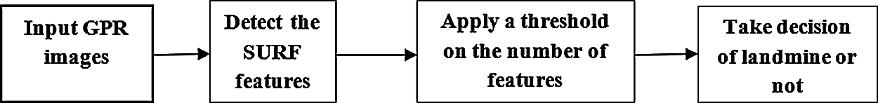
Figure 3: Block diagram of landmine detection with SURF features

The SURF detector-descriptor approach can be considered as a professional alternative to the SIFT descriptor. The SURF algorithm is designed to find blob features. The SURF descriptor is faster and more robust than the SIFT descriptor [20,21]. The computation for the detection step of feature points is based on a two-dimension box filter. It uses a scale-invariant blob detector based on the determinant of the Hessian matrix for both scale selection and localization. It takes the approximations of the second-order Gaussian derivatives using a set of box filters. The Hessian determinant approximation represents the blob response in the image. The 9 × 9 box filters are used to approximate a Gaussian kernel with σ = 1.2 as the minimum scale for computing the blob response representations. These approximations are referred toasDxx, Dyy, andDxy, while the Hessian determinant approximation can be written as [22]:

Det(Happrox)=Dxx−(wDxy)2(7)

where w is a comparative weight for the filter response, and it is used to balance the Hessian determinant expression. These responses are stored in a blob response map, and local maxima are detected and refined using quadratic interpolation and the DoG. Finally, we do non-maximum suppression in a 3 × 3×3 neighborhood to get steady interest points and the scale of values.

The SURF descriptor starts by constructing a square region centered around the detected point and oriented along with its main orientation. The size of this window is 20 s, where s is the scale at which the point is detected. Then, the region of interest is further divided into smaller 4 × 4 sub-regions and for each sub-region [22], the Haar wavelet responses in the vertical and horizontal directions (denoted as dx and dy, respectively) are computed at the 5 × 5 sampled points as shown in Fig. 4.

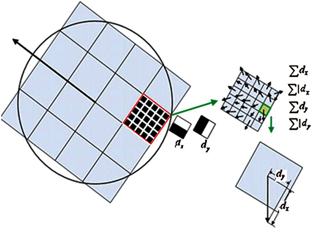
Figure 4: Dividing the region of interest into 4 × 4 sub-regions for computing the SURF descriptor

These responses are weighted with a Gaussian window centered at the interest point to increase the robustness against geometric deformations and localization errors. The wavelet responses dx and dy are summed up for each sub-region and entered in a feature vector v, where [21]

v=[∑⁡dx,∑⁡|dx|,∑⁡dy,∑⁡|dy|](8)

Computing this for all 4 × 4 sub-regions, the resulting feature descriptor of length 4 × 4×4 = 64 is obtained. Finally, the feature descriptor is normalized to a unit vector in order to reduce illumination effects [23]. Finally, after detecting the feature points of the GPR images, a threshold can be set based on the number of feature points. This threshold can be used to test the image if it contains a landmine or not.

4  Efficient Storage of Landmine Images

This section presents an approach for saving the storage area of landmine images based on decimation and interpolation at the detection stage. This approach aims to reduce the size of the landmine database, while maintaining the ability to detect landmines if the images are interpolated.

The acquisition and storage of landmine images consume a large storage area, especially if High Resolution (HR) images are stored. This dilemma can be solved if we could find an efficient tool to reduce the storage size of landmine images, while keeping the discriminative features of these images. If we think of image compression, some information loss takes place as a result of compression. An alternative to this solution is to adopt the decimation strategy of images to reduce the storage size. The decimation by two of an image in both directions leads to one-fourth of the original image size. Now, the question is how to recover the original image size if we decided to perform a landmine detection process after extracting the image from the database. There is a need to think of sophisticated solutions for this problem based on interpolation theory. To understand this idea, there is a need to explore the decimation process, firstly.

4.1 Decimation Model

Assume that there is an HR GPR image represented as f, which is a lexicographically-ordered vector. To get an LR version g of this image through the decimation process, there is a need to multiply f by the decimation operator D as follows [24–31]:

g=Df(9)

where D is the decimation operator that converts the HR image to an LR image. It is represented as [24–31]:

D=D1⊗D1(10)

while the symbol ⊗ represents the Kronecker product, andD1 is a filtering and down-sampling operator. In the case at hand [24–31],

D1=12[1100⋯000011⋯00⋮⋮⋮⋮⋱⋮⋮0000⋯11](11)

The filtering and down-sampling process is described as shown in Fig. 5 as the HR image is filtered by a horizontal low pass filter, and the output is filtered by a vertical low pass filter to give the desired LR image.

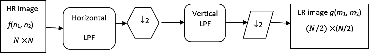
Figure 5: Filtering and down-sampling from an HR image of a size N×N to an LR image of size (N/2)×(N/2)

4.2 Image Reconstruction Using Interpolation Techniques

Image reconstruction before landmine detection from the stored LR images is a necessary task. Reconstruction can be performed as an inverse process of the decimated version using interpolation techniques [26]. This can be performed with maximum entropy or regularized interpolation techniques, as shown in Fig. 6. The objective is to reconstruct the images with as many discriminative features as those of the original images prior to decimation.

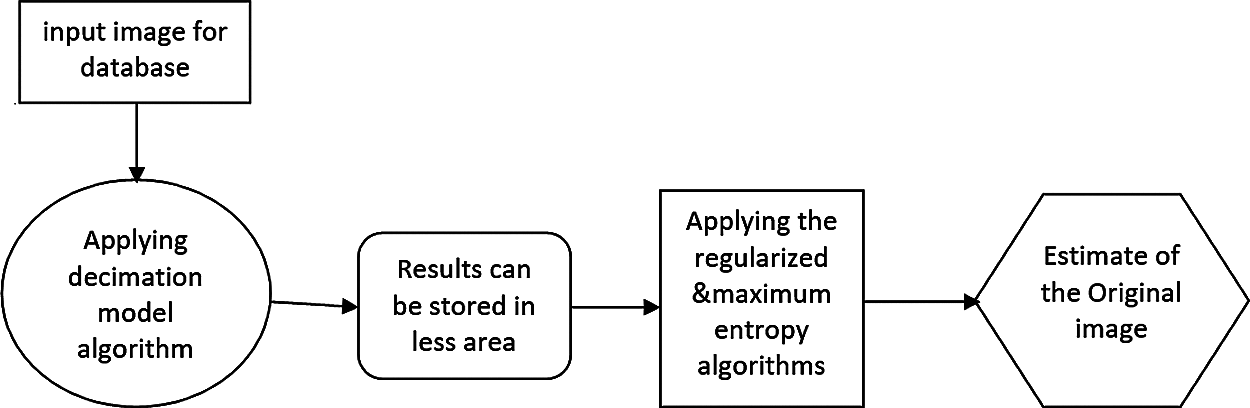
Figure 6: Proposed decimation/interpolation algorithm

4.2.1 Maximum Entropy Interpolation

This approach is based on obtaining an image with maximum entropy. The entropy [27–31] of the image is defined as follows:

He=−∑i=1N2filog2(fi)(12)

We can consider normalized pixel values as probabilities in the image and find the entropy in vector form as follows:

He=−ftlog2(f)(13)

We have to maximize the entropy subject to the constraint that [27–31]:

||g−Df||2=||v||2(14)

We need to minimize this cost function:

Ψ(f)=ftlog2(f)−λ[||g−Df||2−||v||2](15)

where λ represents a Lagrangian multiplier.

In the previous equation, by using the differentiation of the two terms with respect to f, and then equating the final result to zero:

∂Ψ(f)∂f=0=1ln⁡(2){1+ln⁡(f^)}+λ[2Dt(g−Df^)](16)

By solving, we get:

ln⁡(f^)=−1−λln⁡(2)[2Dt(g−Df^)](17)

Then:

f^=exp⁡[−1−λln⁡(2)[2Dt(g−Df^)]](18)

By the usage of Taylor expansion in order to expand the result, and neglecting all but the first two terms, while g−Df^ must be a small quantity, this results in the following equation:

f^≅−λln⁡(2)[2Dt(g−Df^)](19)

Solving for f^, the result will be:

f^≅(DtD+ηI)−1Dtg(20)

and η=−1/(2λln⁡(2)). If the direct inversion is applied to (DtD+ηI), and due to the nature of this sparse diagonal matrix, the inversion process can be simply performed. The diagonal matrix DtD refers to interpolation after decimation.

4.2.2 Regularized Image Interpolation

There is another solution to solve the ill-posed interpolation problem through regularization theory by setting some constraints on the smoothness of the image to be obtained [32–34]. The cost function to be minimized in this case is given as [31,32]:

Ψ(f^)=||g−Df^||2+λ||Qf^||2(21)

where Q is the 2-D regularization operator, and λ is the regularization parameter.

Applying the derivative to the cost function results in:

∂Ψ(f^)∂f^=0=2Dt(g−Df^)−2λQtQf^(22)

This leads to the following solution [29–31]:

f^=(DtD+λQtQ)−1Dtg(23)

An iterative solution for the estimation is possible in this case as follows:

fi+1=fi+η0{Dtg−(DtD+λQtQ)fi}(24)

5  Simulation Results

5.1 Gauss Gradient Results

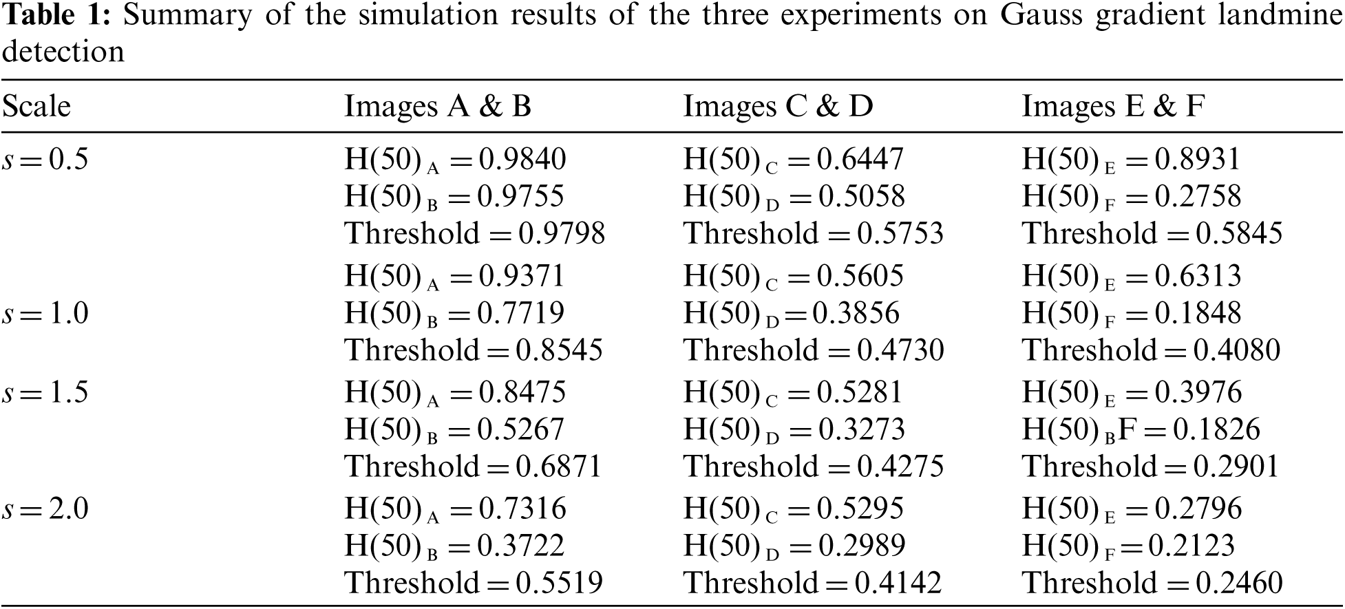
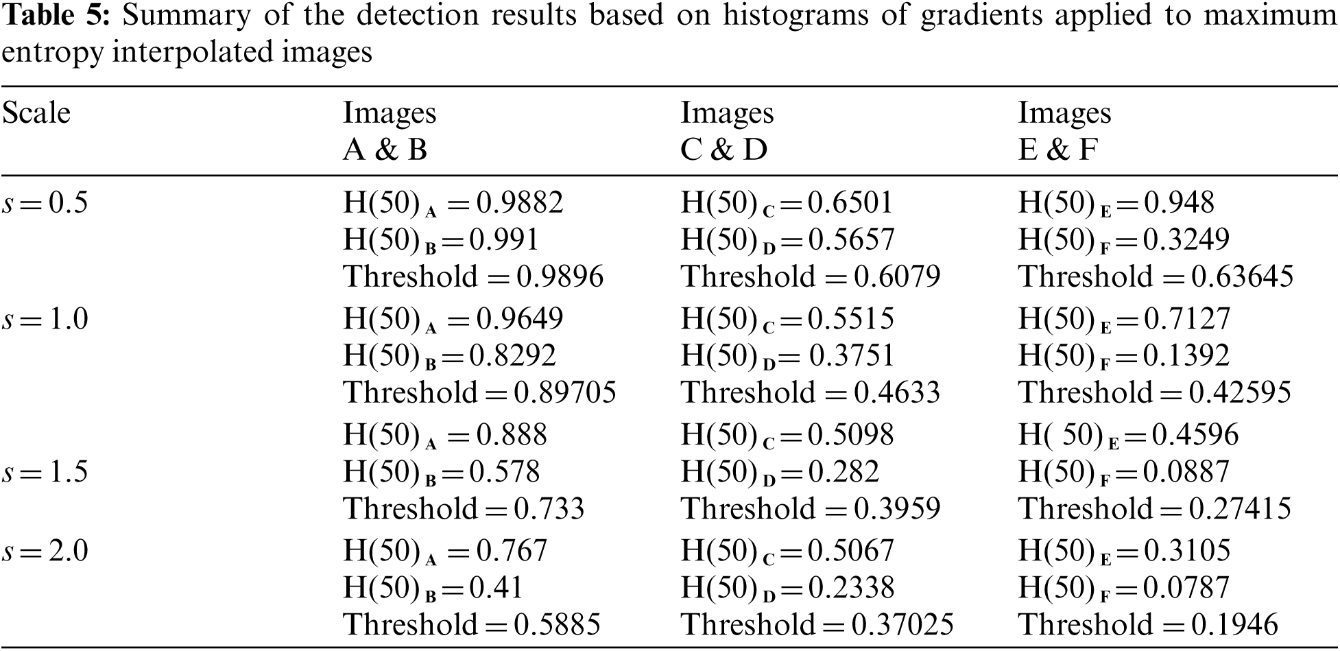
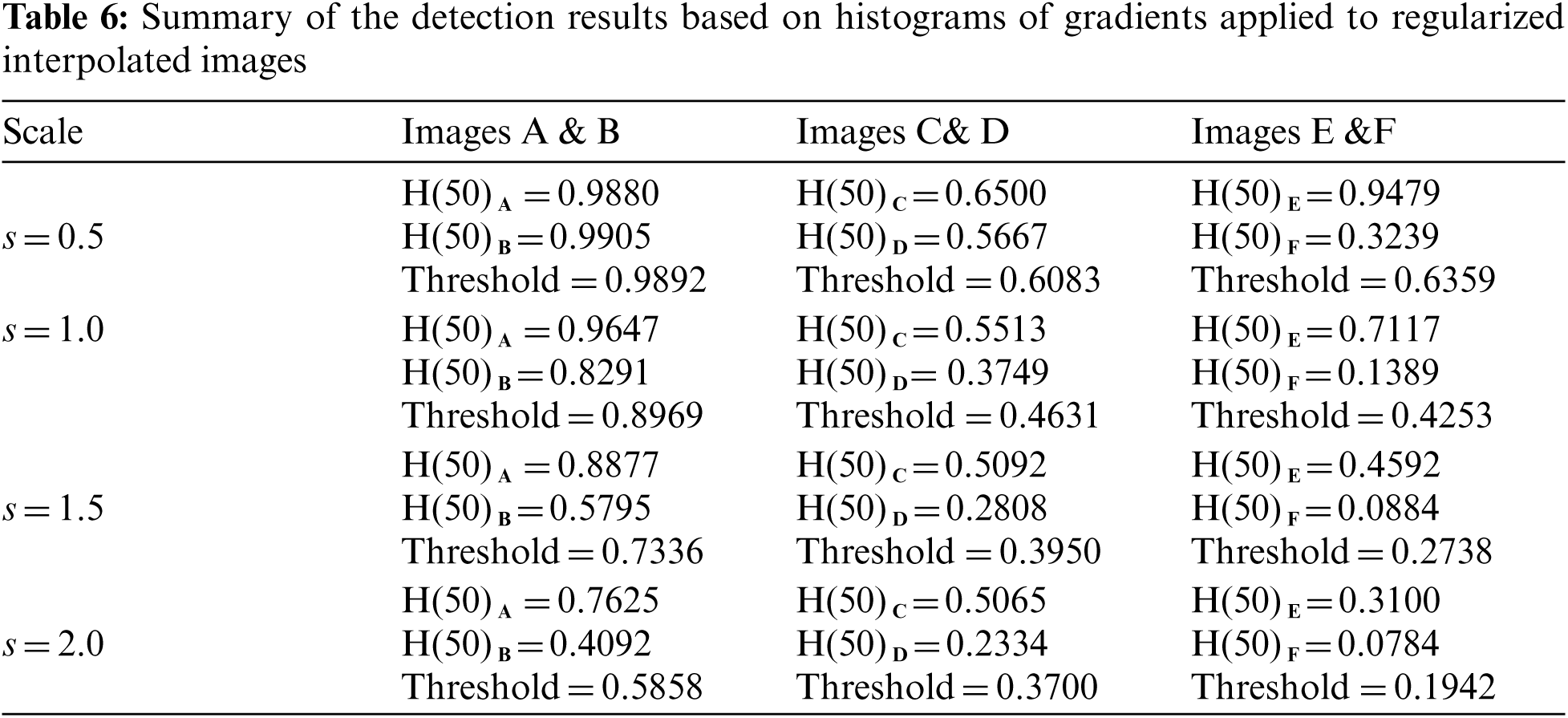
Three simulation experiments have been conducted to detect landmines from GPR images. Two images have been used in each experiment: one with a landmine and the other without a landmine. The strategy in all experiments is to apply the Gauss gradient first on both images, and after that, a histogram is estimated for the obtained gradient for each image. Finally, the cumulative histogram is estimated for each case. The results of these experiments are shown in Figs. 7 to 28. A careful look at the cumulative histogram curves reveals that the images with landmines always have more edges, and the cumulative histograms of their edges rise up to the target value of one with a higher rate of change. Thus, it is possible to select a gray level of 50, for example, and threshold the cumulative histogram of the Gauss gradient at this level to use it for discrimination between images with landmines and images without landmines. Tab. 1 illustrates these discrimination levels at 50 in each experiment. In scale-space theory, the standard deviation of the Gaussian kernel used is named the scale. The obtained results reveal the dependency of the threshold on the scale of the Gaussian filter. Figs. 7a and 8 show that there is a difference in the obtained gradient images with the scale.

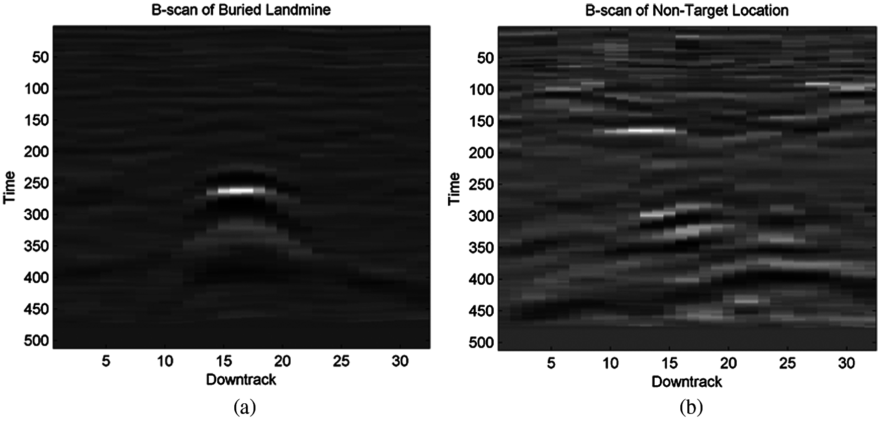
Figure 7: Image (a) with a landmine and image (b) without a landmine

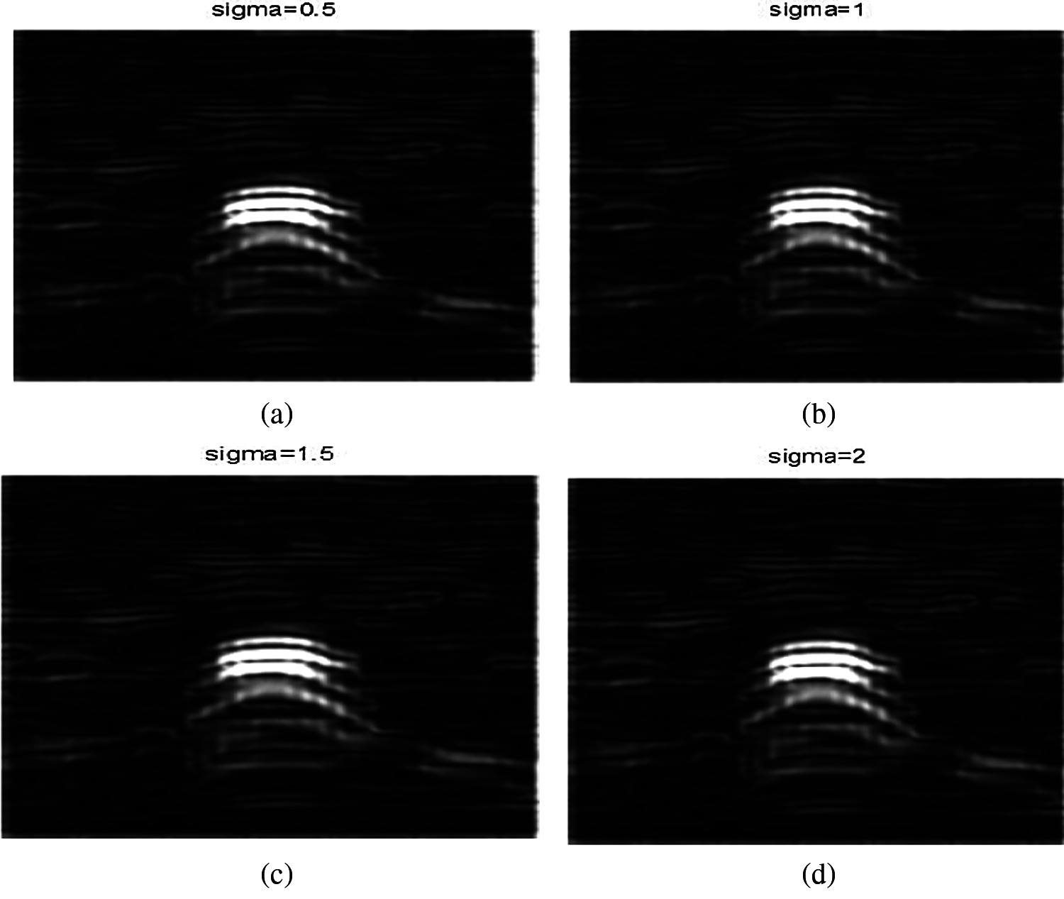
Figure 8: Images after applying Gauss gradient on image A at different standard deviations (scale) values of 0.5, 1, 1.5, and 2 (a) Image A after applying Gauss gradient at standard deviation (scale) 0.5. (b) Image A after applying Gauss gradient at standard deviation (scale) 0.5. (c) Image A after applying Gauss gradient at standard deviation (scale) 1.5. (d) Image A after applying Gauss gradient at standard deviation (scale) 2

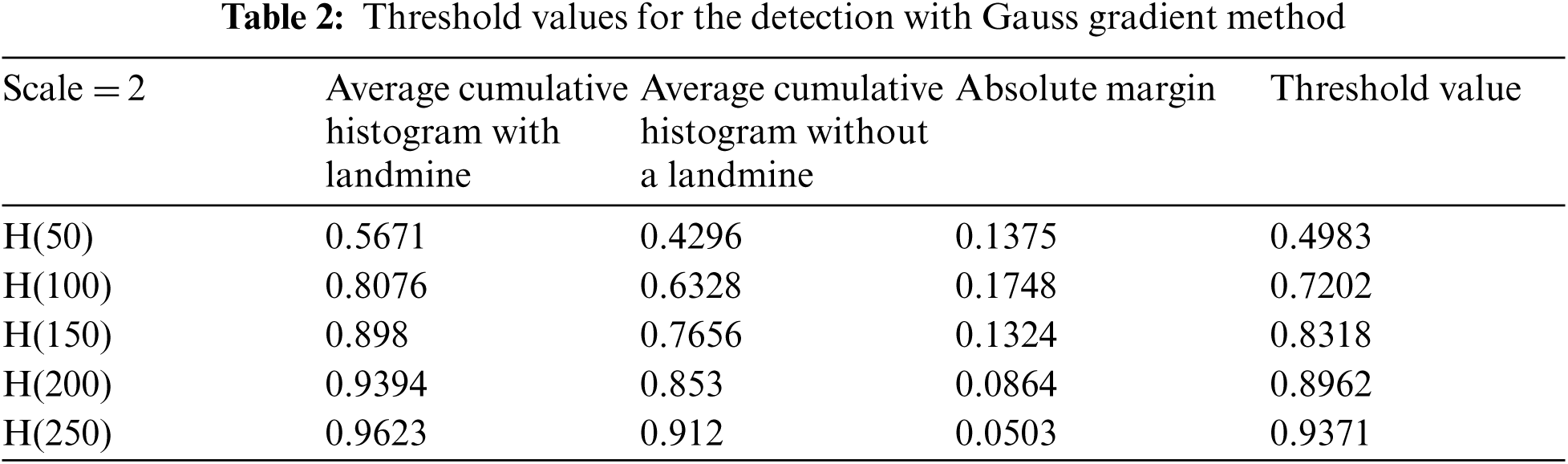
Tab. 1 reveals that the threshold estimated for landmine detection mainly depends on the scale or standard deviation of the Gaussian kernel used. The value of H(50) is selected as there is a clear difference between H(50) with and without landmines. Therefore, we can set a threshold on H(50) to discriminate between images with and without landmines. To follow a general strategy for landmine detection, we can take the average cumulative histogram for the images with landmines and the average cumulative histogram for the images without landmines, as shown in Figs. 9–28. This can help in using all cumulative histogram bins for discrimination, and hence we can estimate accuracy for the detection with any bin.

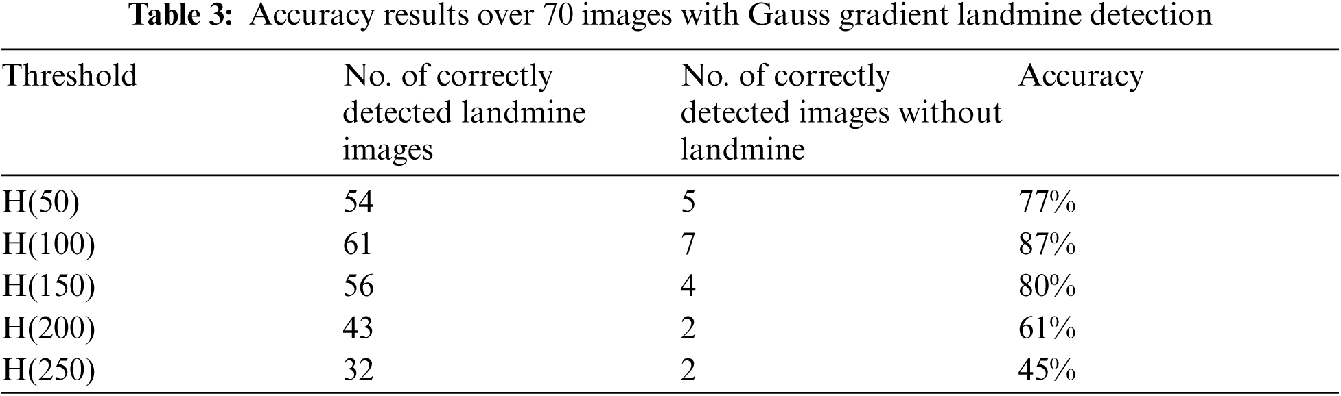
Tabs. 2 and 3 summarize the detection results with different bins of the cumulative histograms. These results show the highest accuracy by working on H(150) is acceptable, and there is some sort of clustering of images with landmines and images without landmines at this bin value.

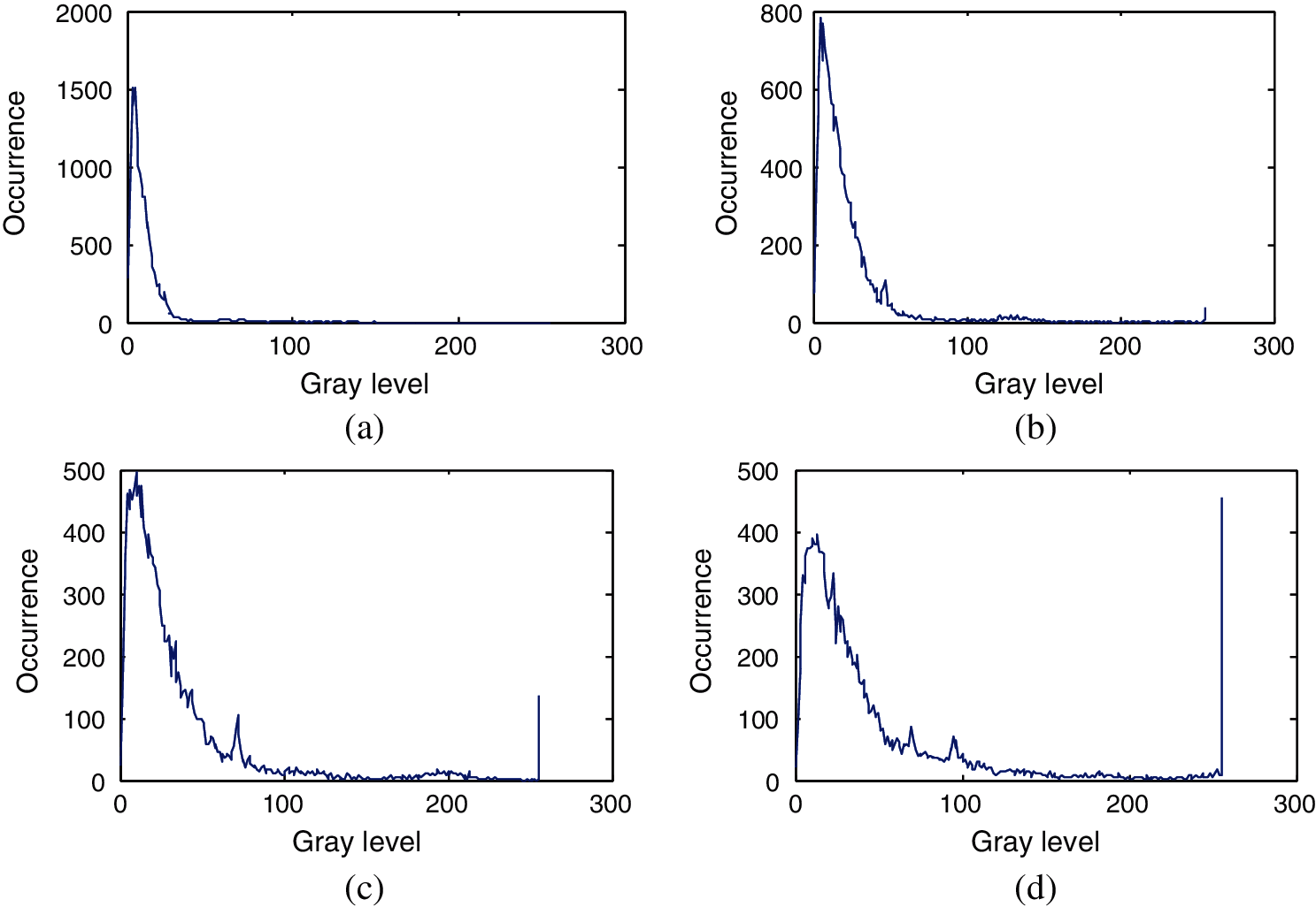
Figure 9: Histograms of the images obtained from image A after applying Gaussian gradient with standard deviations (scale) 0.5, 1, 1.5, and 2 (a) Histogram of image A after applying Gauss gradient with standard deviation (scale) 0.5. (b) Histogram of image A after applying Gauss gradient with standard deviation (scale) 1. (c) Histogram of image A after applying Gauss gradient with standard deviation (scale) 1.5. (d) Histogram of image A after applying Gauss gradient with standard deviation (scale) 2

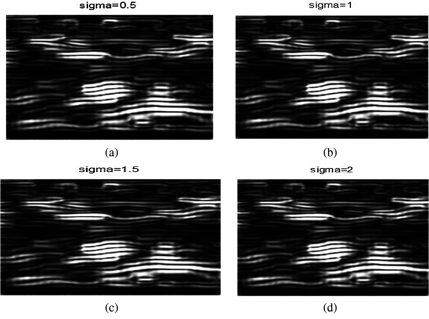
Figure 10: Results of the Gauss gradient method at different standard deviations (scales) (a) Image B after applying Gauss gradient at standard deviation (scale) 0.5. (b) Image B after applying Gauss gradient at standard deviation (scale) 1. (c) Image B after applying Gauss gradient at standard deviation (scale) 1.5. (d) Image B after applying Gauss gradient at standard deviation (scale) 2

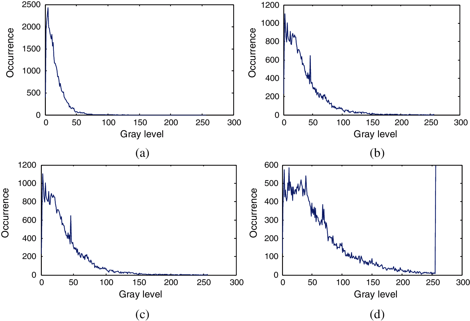
Figure 11: Histograms of the images obtained from image B after applying Gaussian gradient with the standard of deviations (scales) 0.5, 1, 1.5, and 2 (a) Histogram of image B after applying Gauss gradient with standard deviation (scale) 0.5. (b) Histogram of image B after applying Gauss gradient with standard deviation (scale) 1. (c) Histogram of image B after applying Gauss gradient with standard deviation (scale) 1.5. (d) Histogram of image B after applying Gauss gradient with standard deviation (scale) 2

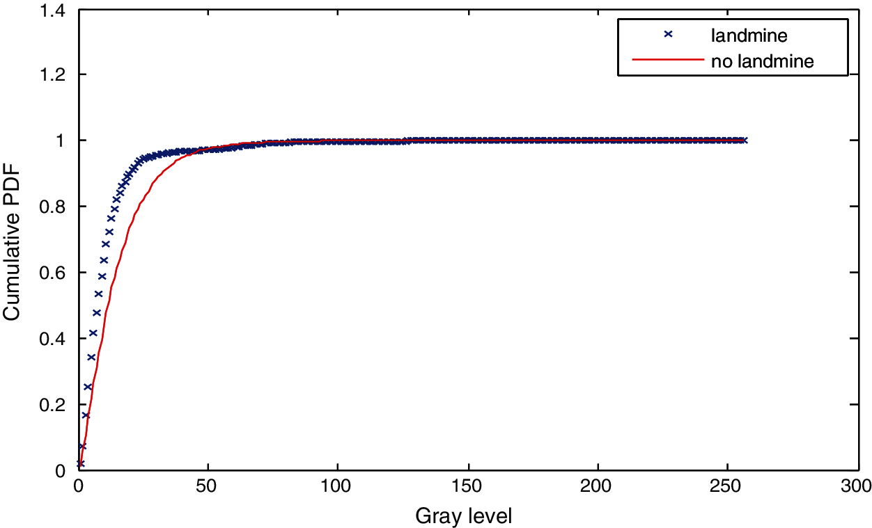
Figure 12: Cumulative histograms of gradients of images A and B at standard deviation (scale) 0.5

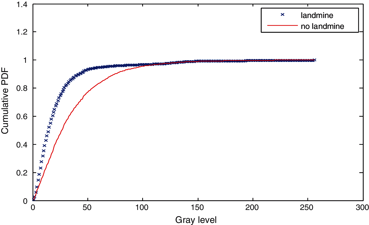
Figure 13: Cumulative histograms of gradients of images A and B at standard deviation (scale) 1

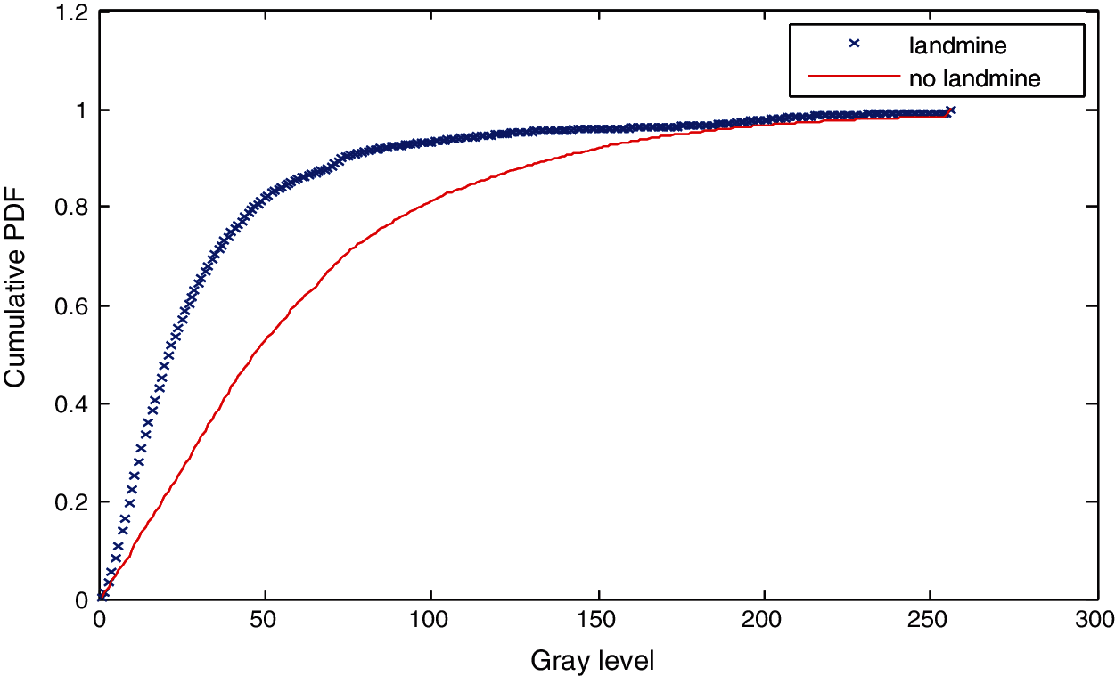
Figure 14: Cumulative histograms of gradients of images A and B at standard deviation (scale) 1.5

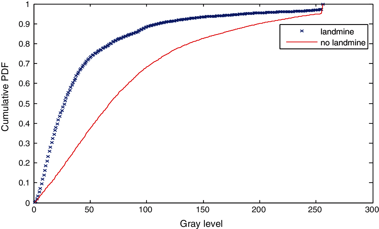
Figure 15: Cumulative histograms of gradients of images A and B at standard deviation (scale) 2

Figure 16: Image C with a landmine

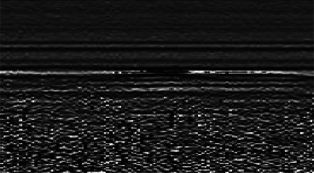
Figure 17: Image D without a landmine

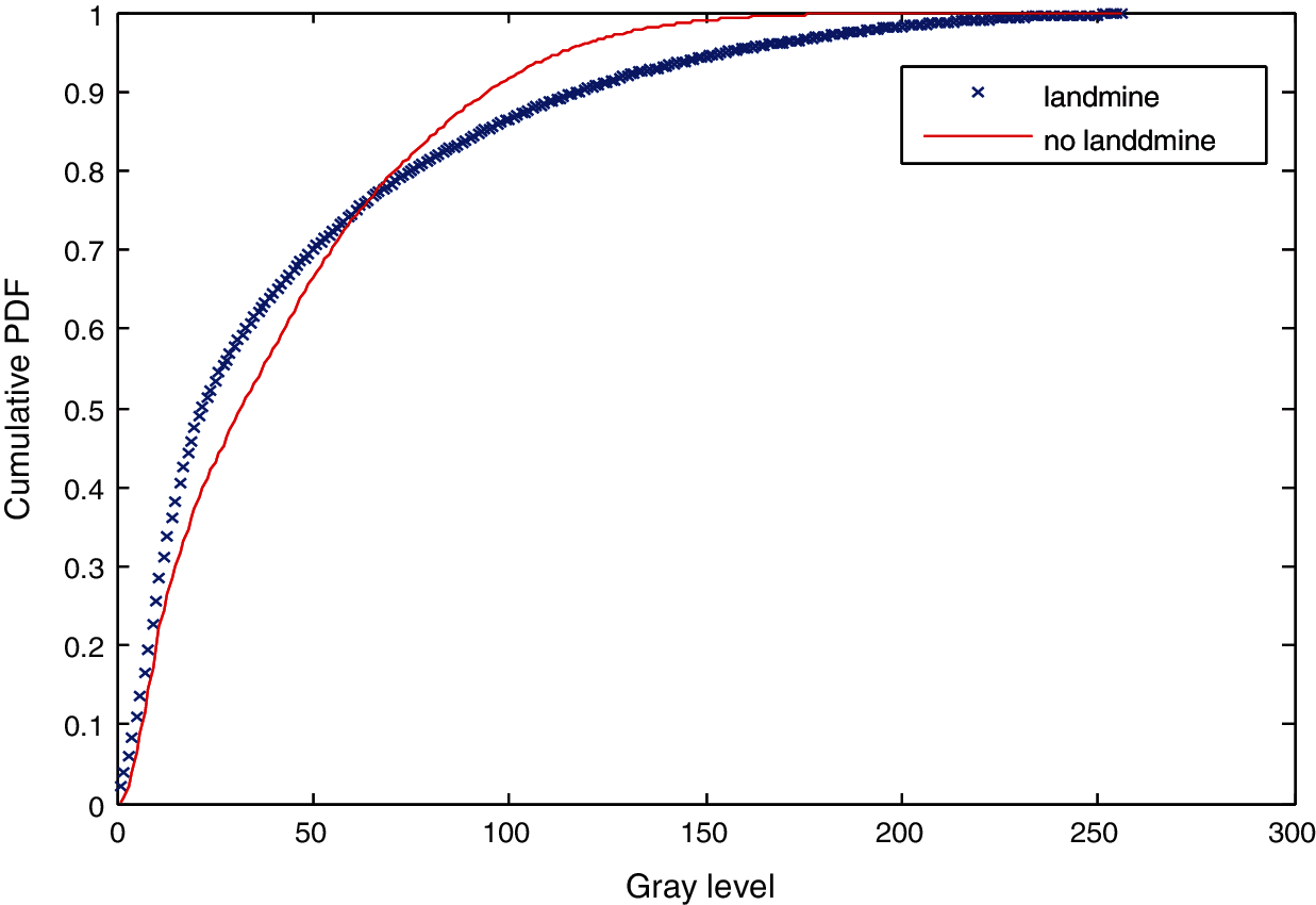
Figure 18: Cumulative histograms of gradients of images C and D at standard deviation (scale) 0.5

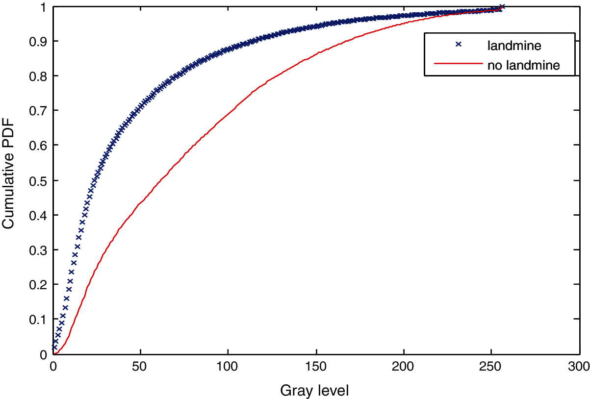
Figure 19: Cumulative histograms of gradients of images C and D at standard deviation (scale) 1

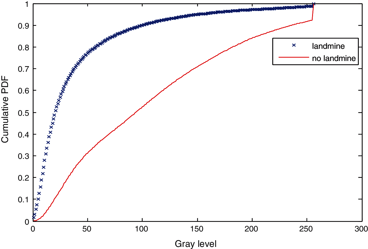
Figure 20: Cumulative histograms of gradients of images C and D at standard of deviation (scale) 1.5

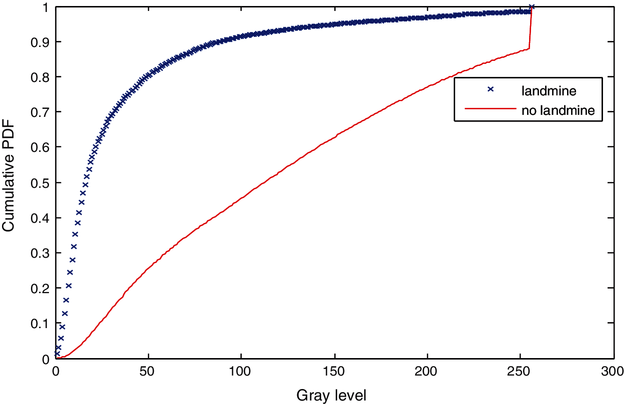
Figure 21: Cumulative histograms of gradients of images C and D at standard deviation (scale) 2

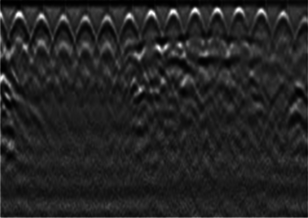
Figure 22: Image E with a landmine

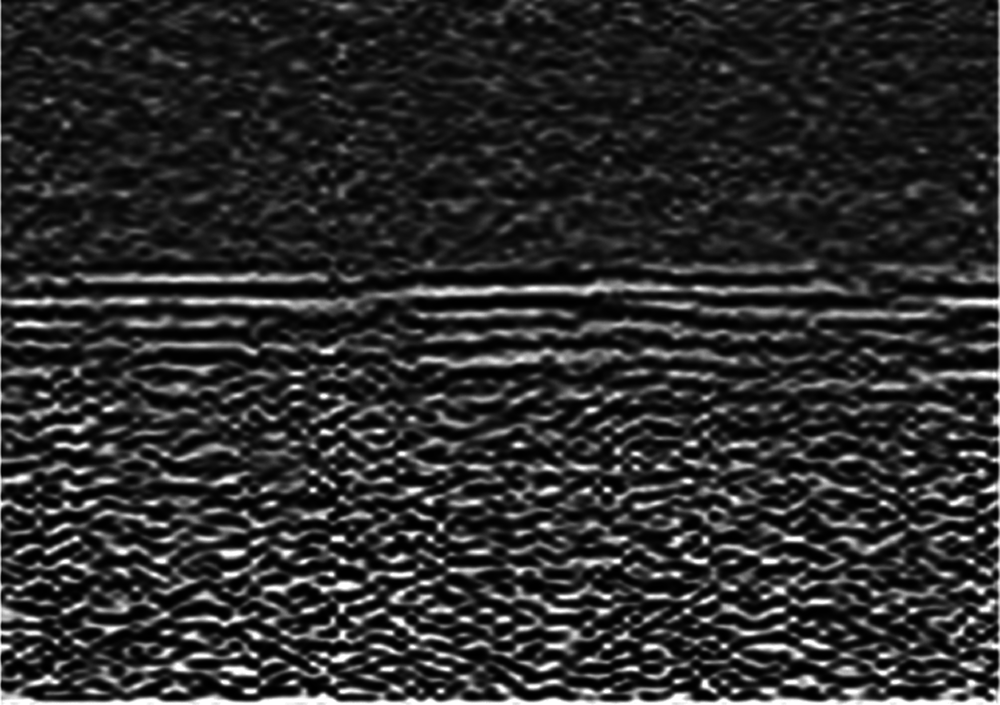
Figure 23: Image F without a landmine

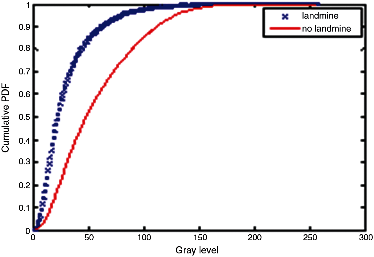
Figure 24: Cumulative histograms of gradients of images E and F at standard deviation (scale) 0.5

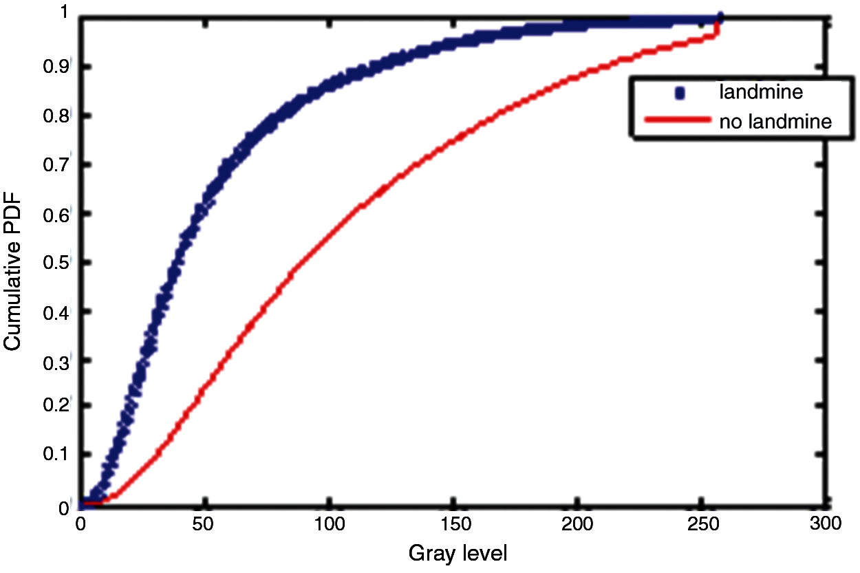
Figure 25: Cumulative histograms of gradients of images E and F at standard deviation (scale) 1

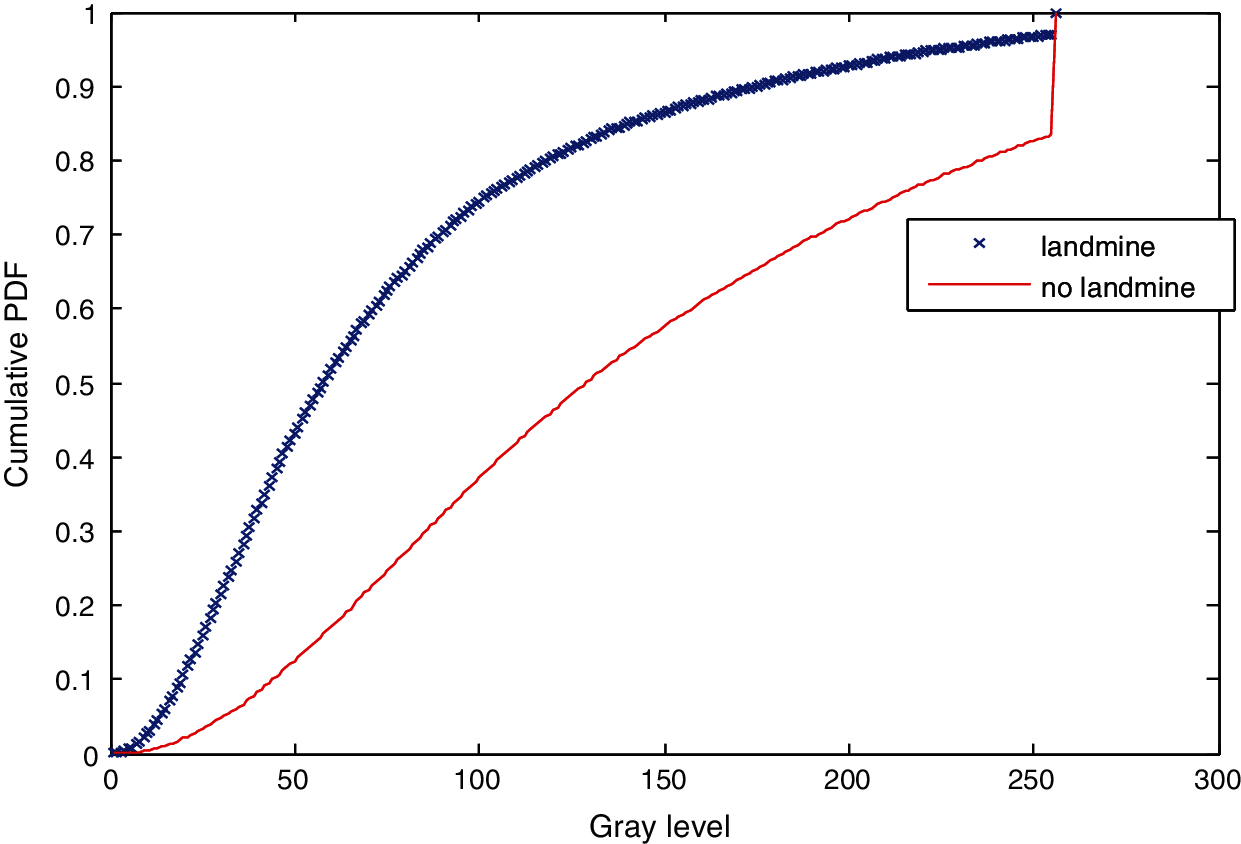
Figure 26: Cumulative histograms of gradients of images E and F at standard deviation (scale) 1.5

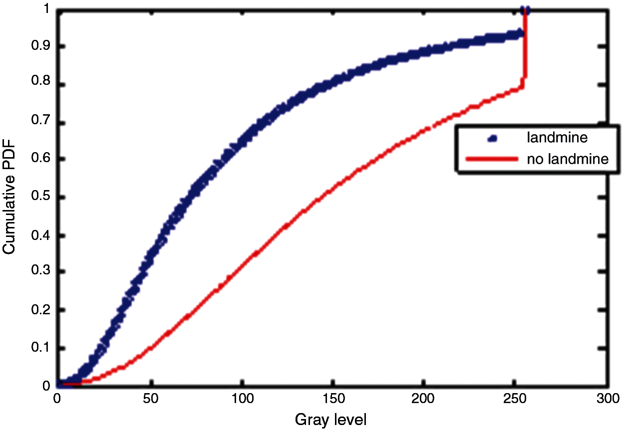
Figure 27: Cumulative histograms of gradients of images E and F at standard deviation (scale) 2

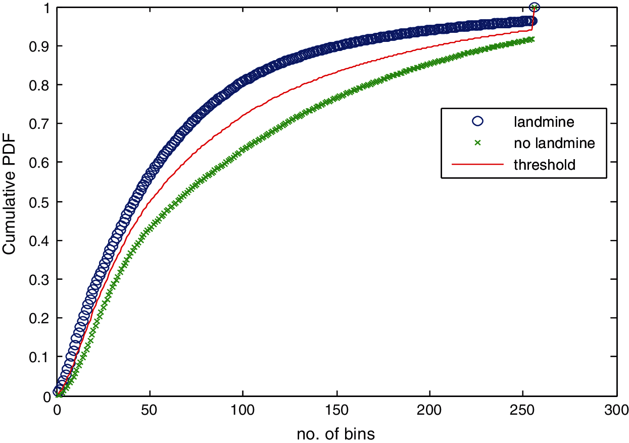
Figure 28: Average cumulative histograms for images with landmines and images without landmines

5.2 Results Based on Neural Classification

Instead of using a thresholding process for the detection of landmines, we can train a neural classifier with specific bins of the cumulative histograms of gradients for images with and without landmines. The number of input nodes can be variable based on the selected margin of the cumulative histogram. For example, if we select the margin from H (50) to H(150), we can have 101 inputs in the input layer. Thus, a single hidden layer is enough for the classification. The classification accuracy of the neural classifier reaches 89%, which is better than the values obtained with a single bin from the cumulative histogram. Fig. 29 shows the convergence performance of the neural network.

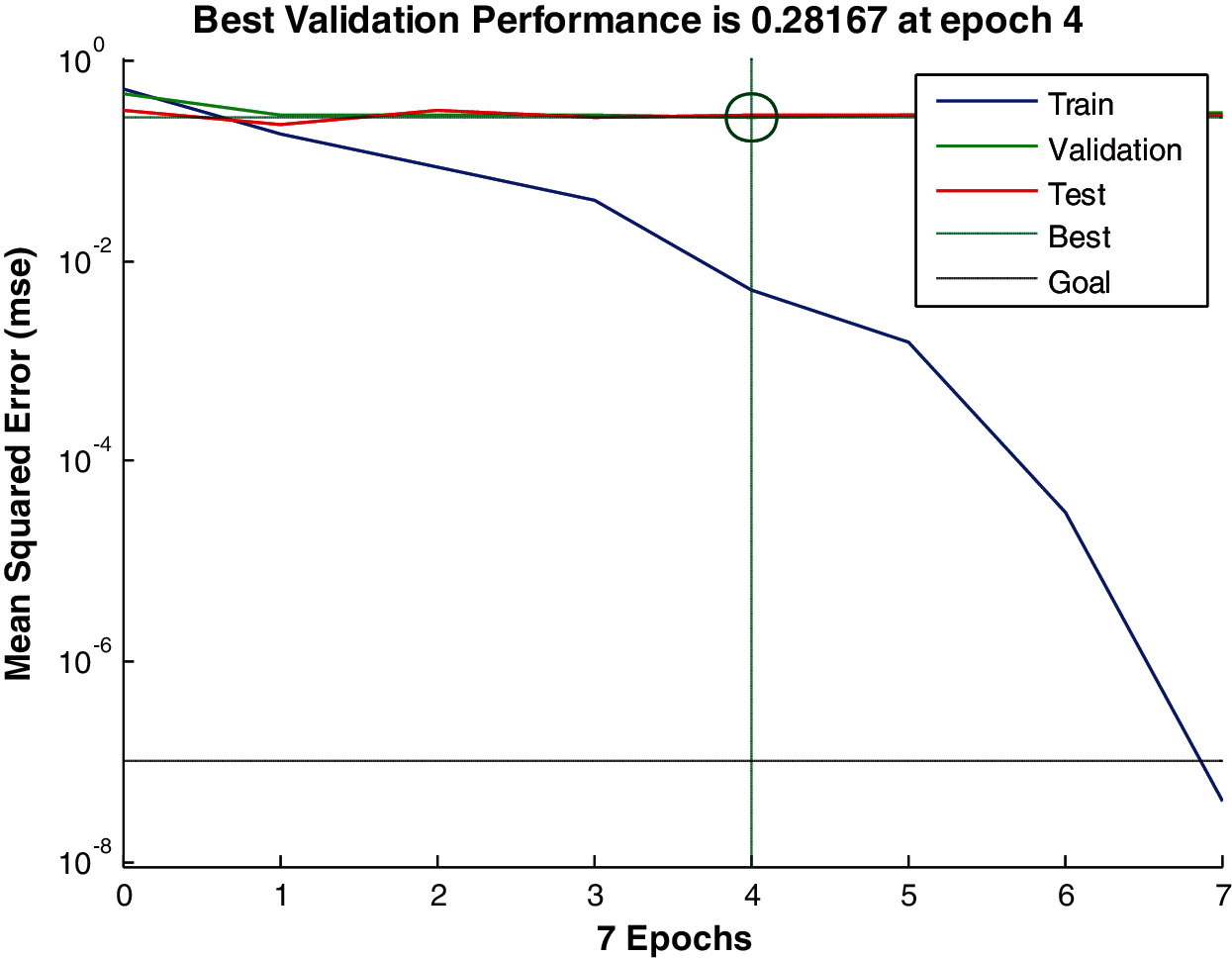
Figure 29: Convergence performance of the neural network

5.3 Simulation Results for SURF Algorithm

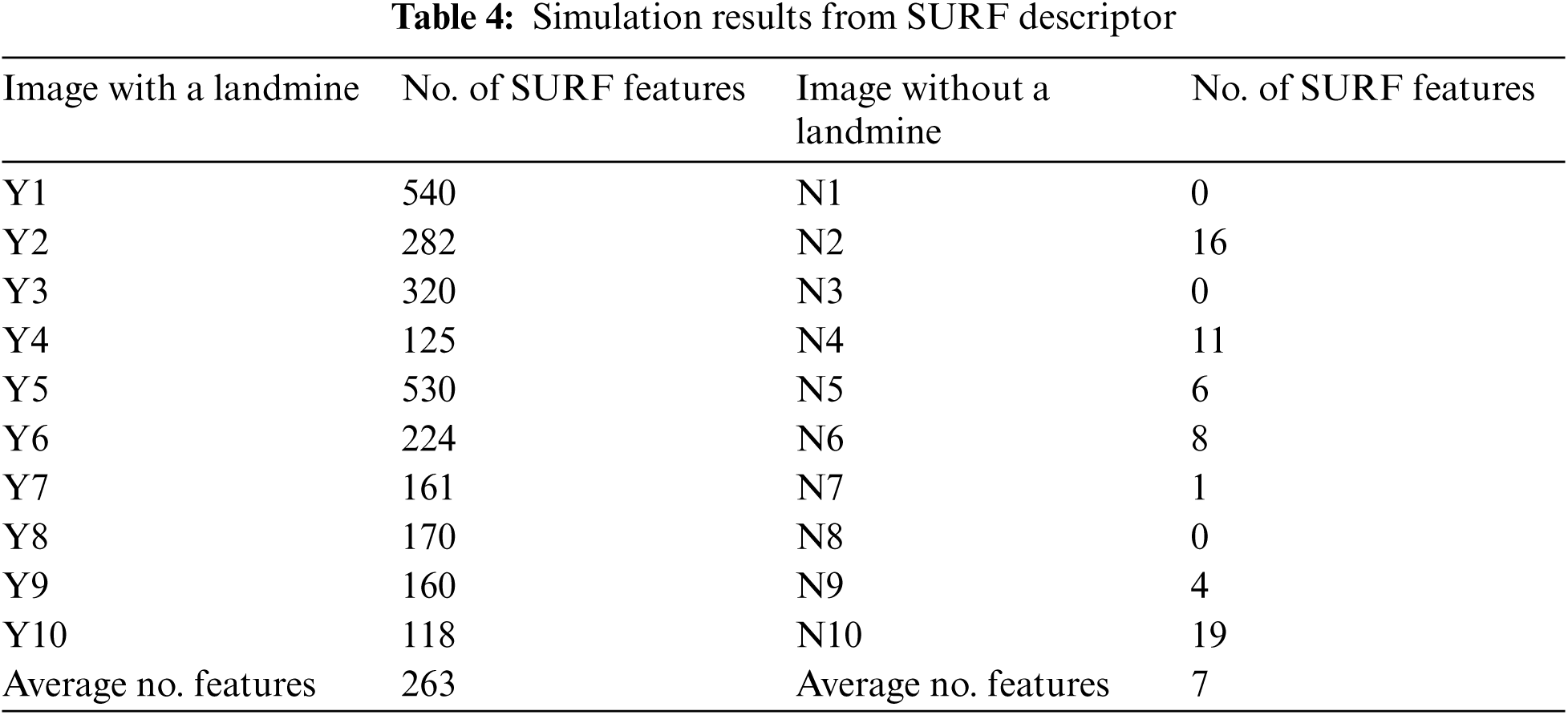
The basic idea of discrimination of landmine images is to detect SURF feature points and count them. A similar process is performed for images without landmines. Figs. 30 and 31 illustrate this process on an image with a landmine. Tab. 4 summarizes the average number of SURF feature points for images with and without landmines. It is clear that a threshold of 135 feature points can be used to discriminate between the images with and without landmines based on the averages obtained in Tab. 3. From these results, we can conclude that the SURF-based classification is more powerful than the technique based on the cumulative histogram of gradients. Thus, we deal with the problem of landmine detection from a different perspective, which is the number of distinguishing points.

Figure 30: Image with a landmine

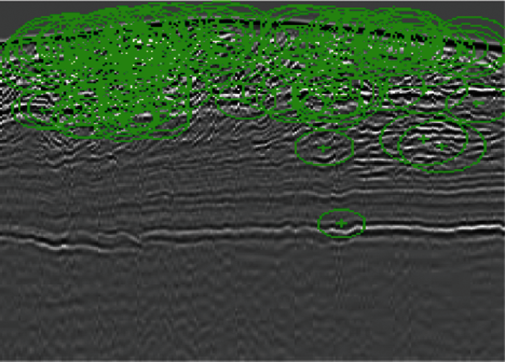
Figure 31: SURF features of the image with a landmine

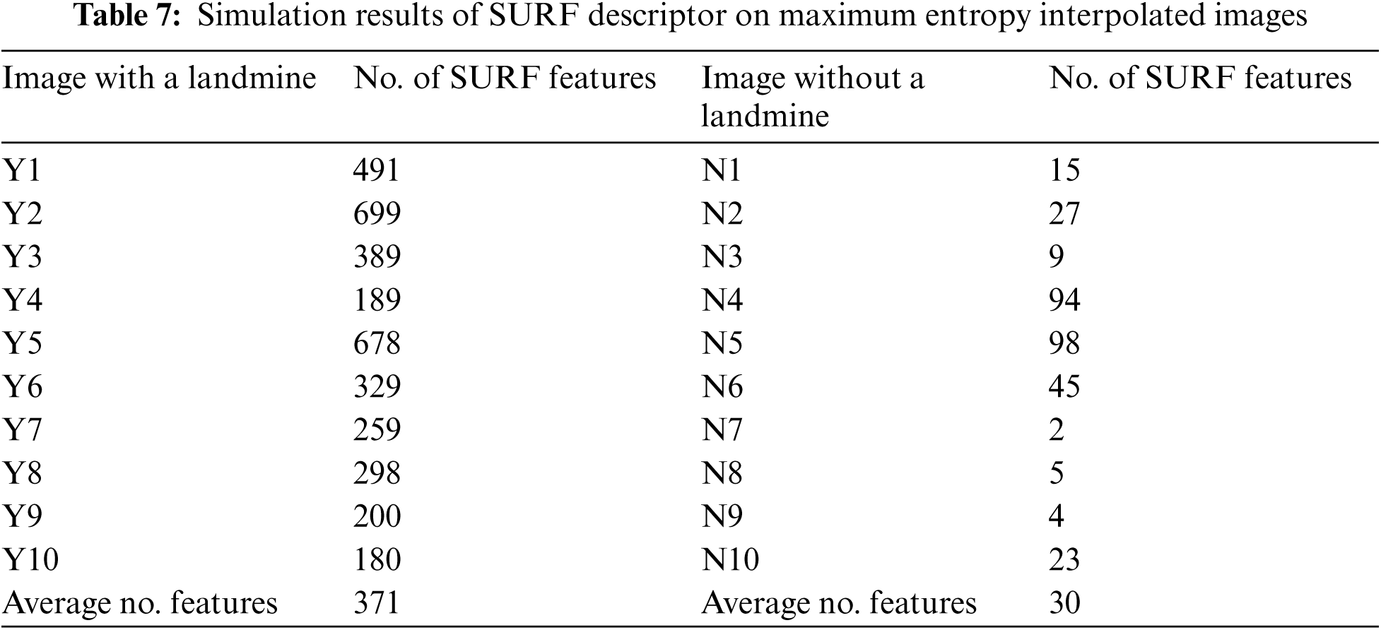
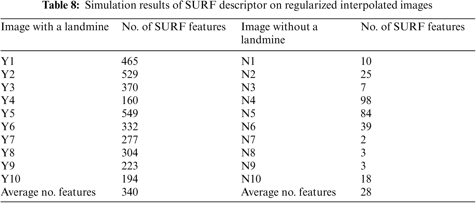
5.4 Sensitivity of Landmine Detection to Decimation and Interpolation

As mentioned in the previous sections, the objective of the decimation process is to reduce the storage size of landmine images. Prior to landmine detection, the interpolation process is performed to restore the original image size. It is required that the interpolated images should have the same features as the original landmine images. Figs. 32 and 33 ensure this fact. It is clear from Tabs. 5–8 that the detection results are not sensitive to the decimation and interpolation results. Thus, it is possible to store GPR images after applying a decimation process to them. Furthermore, the PSNR values after the interpolation process are high enough to reconstruct the images with high quality. The simulation results of these tables reveal that although we have performed decimation and interpolation, it is still possible to discriminate between images based on the number of points extracted from the SURF algorithm.

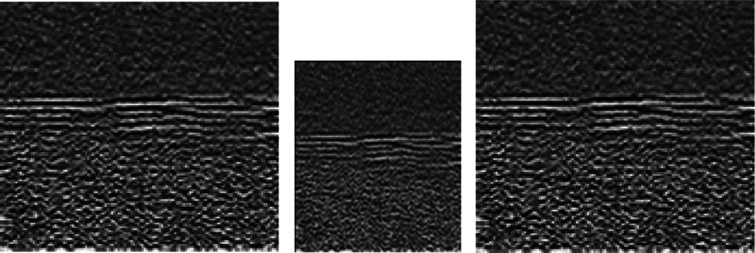
Figure 32: Decimation and maximum entropy estimation of a GPR image with PSNR = 33.48

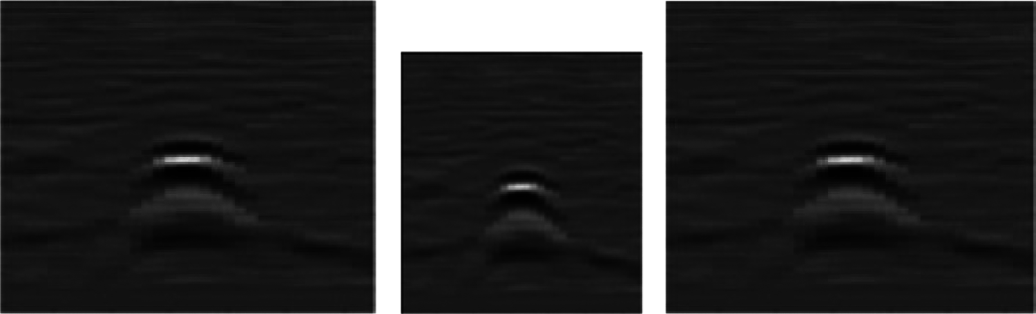
Figure 33: Decimation and regularized estimation of a GPR image with PSNR = 41.038

6  Conclusions

This paper has dealt with a vital image processing problem, which is detecting landmines from GPR images. This task is very important for the demining efforts without victims. The paper presented two basic trends for landmine detection from the GPR images. The first trend depends on the estimation of the cumulative histograms of gradients of images. Simulation results have revealed that it is possible to discriminate between images with and without landmines if a certain gray level is adopted and a threshold is set for discrimination on the cumulative histogram curves. The simulation results have also proved that the selected threshold is scale-dependent. A proper structure of a neural classifier that comprises one input layer consisting of one input, one hidden layer, and one output node can be used for the classification task. The bin values of the cumulative histograms are used as inputs to the neural network for training and testing. Simulations considering a neural classifier showed a promising landmine detection performance with a 92% success rate. This result reflects the possibility of detecting landmines with histogram bins. Some missing landmines are attributed to the close values of bins at the start and end of cumulative histograms of images with and without landmines.

The second approach adopted for landmine detection in this paper is based on scale-space theory and the extraction of SURF features. The idea of this approach is based on estimating the SURF points and adopting the number of these points as a basis for discrimination between images with and without landmines. Simulation results have revealed that the images with landmines have significantly large numbers of SURF features compared to the images without landmines. Selecting an appropriate threshold for the number of SURF points can make the detection process easy with a success rate of 100%. No false alarms have been recorded with this approach.

Another issue that has been studied in this paper is the storage of landmine images. To reduce the storage size of landmine images, decimation by two can be adopted for this purpose. This leads to a 75% reduction in the storage space for landmine images. An interpolation scheme can be used to reconstruct the landmine images with their original sizes prior to any landmine detection process. Simulation results have revealed that landmine detection is not affected by the decimation and interpolation processes. In future work, different algorithms based on the utilization of artificial intelligence tools are recommended for accurate landmine detection. Also, we intend to utilize more advanced signal processing techniques for the efficient compression of landmine images.

Acknowledgement: The authors would like to thank the support of the Deanship of Scientific Research at Princess Nourah bint Abdulrahman University.

Funding Statement: This research was funded by the Deanship of Scientific Research at Princess Nourah Bint Abdulrahman University through the Fast-track Research Funding Program.

Conflicts of Interest: The authors declare that they have no conflicts of interest to report regarding the present study.

This work is licensed under a Creative Commons Attribution 4.0 International License, which permits unrestricted use, distribution, and reproduction in any medium, provided the original work is properly cited.