DOI:10.32604/cmc.2022.021492
| Computers, Materials & Continua DOI:10.32604/cmc.2022.021492 | |
| Article |
Parking Availability Prediction with Coarse-Grained Human Mobility Data
1University of Murcia, Murcia, 30003, Spain
2Universidad Católica de Murcia (UCAM), Murcia, 30107, Spain
*Corresponding Author: Fernando Terroso-Sáenz. Email: fterroso@ucam.edu
Received: 04 July 2021; Accepted: 14 October 2021
Abstract: Nowadays, the anticipation of parking-space demand is an instrumental service in order to reduce traffic congestion levels in urban spaces. The purpose of our work is to study, design and develop a parking-availability predictor that extracts the knowledge from human mobility data, based on the anonymized human displacements of an urban area, and also from weather conditions. Most of the existing solutions for this prediction take as contextual data the current road-traffic state defined at very high temporal or spatial resolution. However, access to this type of fine-grained location data is usually quite limited due to several economic or privacy-related restrictions. To overcome this limitation, our proposal uses urban areas that are defined at very low spatial and temporal resolution. We conducted several experiments using three Artificial Neural Networks: Multilayer Perceptron, Gated Recurrent Units and bidirectional Long Short Term Memory networks and we tested their suitability using different combinations of inputs. Several metrics are provided for the sake of comparison within our study and between other studies. The solution has been evaluated in a real-world testbed in the city of Murcia (Spain) integrating an open human-mobility dataset showing high accuracy. A MAPE between 4% and 10% was reported in horizons of 1 to 3 h.
Keywords: Parking space; human mobility mining; recurrent neural networks; prediction
At the dawn of the smart cities era, municipalities are still facing a lack of proper transportation policies for the efficient management of human mobility. As a result, problems related to road traffic congestion have become challenging issues within urban settlements. In economic terms, it is estimated that traffic jams cost $87 millions in the USA in 20191. Also, traffic congestions have a direct impact on the air quality of a region since petrol vehicles are one of the most important sources of air pollutants [1].
The development of services for parking space management is a sensible solution to reduce traffic-congestion, since roughly 40% of road traffic in cities is caused by drivers searching for parking space2. In that sense, the anticipation of future parking-space demand would allow operators to develop short-term and long-term counteractions to avoid mobility problems in urban regions.
For that prediction, a paramount contextual factor to be considered is the road-traffic conditions of the urban areas. In that sense, a large course of action for parking availability prediction leverages the endless deployment of new and more powerful sensors across cities thanks to the Internet of Things (IoT) [2]. More in detail, mechanisms based on static infrastructure sensors [3], mobile ones [4] or the crowdsensing paradigm [5] have already been proposed. In general terms, these solutions rely on high-resolution mobility data that captures human or vehicle displacements at quite fine-grained temporal or spatial scales. For example, a solution based on mobile sensors mounted on floating vehicles (e.g., taxis or buses) would allow monitoring the state of each road segment.
However, high-resolution human mobility data is quite sensitive in terms of privacy. Its access is rather limited because of regulatory and economic policies [6]. At the same time, the open data movement has promoted the release of an increasing number of human-mobility datasets [7–9]. However, they are usually filtered and pre-processed for anonymization. Hence, open mobility data provides a much lower temporal and spatial resolution than ad-hoc mobility feeds. The development of intelligent systems leveraging such coarse-grained mobility data is still scarce in the domain.
In this context, the present work introduces a novel mechanism to forecast the number of available spaces of a set of urban parking lots in the city of Murcia (Spain). Our system relies on two datasources.
On the one hand, the predictor is timely fed with the sheer number of free spaces in the target parking lots. This is provided by a set of counter sensors installed in the parking lots which are, in turn, part of a wide IoT infrastructure deployed in the city. On the other hand, the system also considers the anonymized human trips co-occurring within the city. Such trips are extracted from a nationwide open mobility dataset released by the Spanish Ministry of Transportation (SMT) considering mobile-phone location data from several telephone operating carriers3. To ensure users’ privacy, trips are defined on a spatial tessellation of the country based on large geographical areas.
These two sources are used to train an Artificial Neural Network (ANN) able to anticipate the values from the IoT counters several hours ahead. Given the sequential nature of the inputs, two types of Recurrent Neural Networks (RNNs) have been evaluated, a LSTM [10] and a GRU [11] one. Both types of architectures can learn long and short-term patterns from a given input sequence but some slight differences in terms of complexity exist between them. Nevertheless, both have been successfully applied to the parking availability prediction problem [12]. Hence, the present work also relies on the hypothesis that the latent human movement of a region provides valuable information about its parking occupancy level so such knowledge should be integrated as part of the prediction system.
It is important to note that the inputs are defined at different spatial scales and sources. The occupancy of the parking lots is extracted from an IoT infrastructure, and, in spatial terms, such data is related to very particular spots within the city. However, the human trips dataset only provides a region-based view of the actual human mobility. Therefore, our solution studies whether human mobility data defined at a very high level gives insight into road-traffic behaviour related to city locations captured by the parking lots’ sensors. Some parking-space predictors incorporate in their pipelines data defined at a coarse spatial granularity such as weather conditions. However, to the best of the authors’ knowledge, there is a scarcity of proposals making use of coarse-grained feeds related to human movement information. This targets an important research gap in the parking availability prediction domain.
Furthermore, our work also brings three important operational benefits with respect to existing solutions. Firstly, we can deploy it in cities without an IoT infrastructure able to capture fine-grained mobility data. Secondly, as a side effect, it can be regarded as a cost-effective mechanism. Finally, our approach relies on pre-anonymized human data so it will limit the privacy concerns among end-users.
The rest of the paper is structured as follows. Section 2 provides an overview of current approaches for parking space prediction from different perspectives. Next, Section 3 puts forward the proposed forecasting mechanism and the main results of the performed experiments are described in Section 4. Finally, the main conclusions and the future work are summed up in Section 5.
This section provides an overview of existing approaches for parking space prediction. We gathered three dimensions of the solutions, their input sources, applied algorithms and the urban service that they provide. Last, we also briefly review the main findings within the human mobility mining discipline.
Sensors, parking meters and crowdsensing are common sources for collecting real-time parking availability.
Regarding static sensors, the mechanisms in [4,13,14] use parking meter data for its prediction. Counting data from parking lots at each moment is used in [15–21] where the available slots are collected every 5–15 min. Infrared and ultrasonic sensors can be used to identify a car in a particular spot [2], as well as Radio-Frequency Identification (RFID) [22] for single vehicles that are provided with a radio frequency tag. Furthermore, ferromagnetic sensors installed under the asphalt are used in [23]. Others works focus on the ticket data collected from a smart-parking system [24]. In terms of communication protocols, some proposals use an energy efficient LoRaWAN channel to transmit the collected data to a centralized repository [25].
Concerning mobile sensors, most works rely on vehicle-mounted devices sensing traffic contextual features [13]. A similar approach is followed in [4] where the GPS traces of the fleet of taxis are used for parking availability monitoring. More generalist ways to collect data use machine vision [26] and car count in order to know the number of free spaces in real-time. In this scenario, crowdsensing focuses mainly on developing smartphone apps to ensure the accuracy of parking information and location [5].
Lastly, weather conditions might affect parking demand at different degrees. For that reason, several works have incorporated this data as part of their input [13,15,20]. Other contextual urban feed that has also used in some works has been Point of Interest (POI) data indicating the density of certain venues like restaurants or bars or schools [20,21], since the POI distribution of a region strongly affects its human mobility patterns [27].
The present work takes as input count-based parking data and weather conditions as other proposals in the literature. Our approach also considers mobile data as input in the form of human mobility flows but its spatial and temporal granularity is much larger than the sources of previous works [4,13]. As a matter of fact, the temporal resolution of the traffic dataset in [4] was fixed to 10 min instead of 1 h as in our case as it is pointed out in Sec. 3.2.1. Furthermore, whilst works based on mobile data rely on street-based reports [4,13] our solution considers the incoming or outgoing human flows of large-scale geographical urban areas. For estimating human flows, other works rely on social media publications (geo-tagged information) [28,29]. Unlike previous proposals, our approach combines datasources of different nature. Those are raw sensor data from the counters installed in the parking lots and transmitted through a IoT infrastructure (see Sec. 3.1). and open data capturing the human flows in the target city at very low resolution. As we have seen, this fusion of raw sensor data and an open mobility feed for parking availability prediction has not been fully explored in the literature.
Different ANN models have been applied for parking demand forecasting. Since this can be regarded as a time-series prediction problem, most works have used different types of Recurrent Neural Networks (RNNs), such as Long short-term memory (LSTM) [14,17,18] models. Moreover, the work in [13] combines a Graph Neural Network (GNN) and a LSTM model so as to also consider the underlying road topology of the target area. Hierarchical GNNs have been also used to predict the availability of different parking lots since they capture well the spatial correlations among different entities [21]. Apart from that, Multi-layer Perceptrons (MLPs) have been also proposed and used as a baseline to compare with other algorithms, especially deep learning algorithms [23,30,31]. GRU and LSTM have been proven to be the best RNN architectures for solving a wide set of sequential data problems [32]. In [12], the GRU architecture achieves better results in nearly all scenarios (4 countries and different exogenous variables) compared to the LSTM version for 6 h-ahead prediction. GRU have also been successfully applied to capture dynamic temporal autocorrelations between several parking lots [33]. In [25], authors proposed a network architecture combining three types of layers, 1D convolutional, a LSTM and three fully connected ones for the prediction task. Also, generative adversarial networks (GANs) that merge spatio-temporal and weather data from different urban datasources have been used [20].
Furthermore, researchers in [15] make use of Markov chain analysis as they assume the Markov property in the context of parking space prediction. Similarly, a continuous-time Markov queue is put forward in [16]. A likelihood maximization approach is applied to deal with the heterogeneity of crowd-sensed data is presented in [5]. Other methods like Kalman filters have been also studied [4]. In addition to that, some proposals have used ensemble-learning algorithms like Random Undersampling Boosts to perform the prediction task [24]. In a similar way, [19] proposes an ensemble model where three different algorithms, Random Forest regressor, Gradient boosting regressor and Adaboost regressor are combined by means of bagging and boosting techniques to provide a final prediction outcome.
In terms of applied models, our proposal has evaluated three different models, MLP, GRU and bi-LSTM ones in order to find the most suitable hand for the task in hand as it is described in Sec. 4.4.2.
Different parking scenarios: research works deal with improving efficiency at closed parking lots which are paid parking lots (both indoors and outdoors), andpen parking lots or ticketing.
As long as the first scenario is concerned, a mechanism to predict the occupancy of three private and public parking lots in the next 60 min in Geneva (Switzerland) is proposed in [15]. A set of 14 parking lots in San Francisco (USA) are used as a use case in [16]. In this case, the future available parking places area provided a time horizon of up to 12 min. In the same city, the proposal in [4] controls on-street parking spaces of 579 road segments. The work in [17] provides a prediction mechanism for a single parking lot in Shenzhen (China) with a prediction horizon of 30 min. In [21] the proposed system was able to provide predictions for a set of different parking lots at Beijing and Shenzhen 15, 30 and 45 min ahead. A holistic IoT infrastructure that able to make predictions of 30 parking locations of Birmingham (UK) is proposed in [18]. Unlike previous approaches, the predictions are given in hour intervals instead of minutes and the same dataset is used for 30-minute time horizons in [19].
Regarding the second group of on-street parking spaces, the work in [13] applies its predictor to a downtown area in Pittsburgh (USA). In [20], the prediction targets an outdoor regulated parking zone in Santander (Spain). In both cases, the prediction horizon is up to 30 min. In [5], the crowd-based prediction mechanism is tested in seven on-street public parking spaces in London (UK). In [14], 3000 on-street parking slots were controlled by the solution to provide predictions up to 30 min ahead. The problema can be shifted from regression to classification [24]. This way, the solution is able to classify the level of service at different on-street parking areas in Madrid (Spain). In [25], the predictor focuses on a street in the city of Montova (Italy) providing parking lots prediction from 1 to 8 h ahead.
Our work forecasts the available parking places of two public garages with a larger time granularity (hour vs. minutes) and a wider time horizon of the prediction, as is stated in Sec. 4.4.2.
Human mobility repeats over time (e.g., people tend to go to work at the same time every working day) so it is usually modeled as a time pattern highly predictable at some extend [34]. The prediction of where and when people are going to move is an instrumental tool in many domains [35].
Nowadays it is possible to capture location data at multiple spatial and temporal scales from a large palette of technologies like GPS, Bluetooth or WiFi. Based on these technologies, a variety of machine learning models have been proposed for human mobility forecasting [36]. These solutions basically rely on the raw spatio-temporal trajectories from moving entities, like taxis or individuals, equipped with the location technologies. This allows collecting their current location every few minutes or even seconds.
In this context, human mobility patterns have already been successfully extracted from such open feeds and used in different predictive problems [37]. However, there is a scarcity of proposals leveraging such mobility coarse-grained feeds as reliable input sources to improve other predictive tasks.
This section describes the urban scenario for testing our approach. In that sense, we describe the available data sources and their suitability as input features for parking availability prediction.
The feasibility of our solution has been evaluated in Murcia, a city in the South-East of Spain. Fig. 1 depicts the target urban area within this city. The city of Murcia is involved in a holistic smart-city project called MiMurcia4 that is developing a platform that interconnects data and services to provide citizens with personalised and updated information about the status of the city and to make it smart. Murcia is a city with a great trajectory in the use of IoT data for providing smart services such as water [38] and energy management [39]. Within this platform, several data is published: irrigation, problems reported by citizens (with pictures) and the parking and weather information that our solution uses.
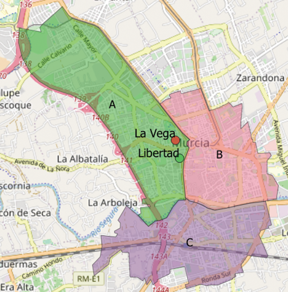
Figure 1: Map of the target city. Each colored polygon is a particular Mobility area from the mobility study whereas the dots indicate the locations of the two target parking lots
Our solution would eventually enrich this ecosystem with a decision-support system for road traffic management. This way, it would provide drivers with real-time information about the available parking spaces in their destination areas on the basis of their time of arrival to such destinations.
Given the urban infrastructure described in the previous section, we focused on the following data sources related to the city to perform the prediction task.
3.2.1 Low-Resolution Human Mobility
As it was mentioned in Sec. 1, we used the nationwide human mobility dataset released by the SMT in December 2020. This dataset covers a 9-month period from February 29th to November 30th, 2020, and it indicates the number of trips among 3216 ad-hoc administrative areas (hereby Mobility Areas, MA) per hour in Spain both in its peninsular and insular extension. In that sense, a single trip stands for the spatial displacement of an individual with a distance above 500 meters. Consequently, this dataset can be regarded as a set of tuples taking the form ⟨date, hour, morigin, mdest, ntrp⟩, reporting that there was ntrp human trips from the MA morigin to mdest during the indicated date and hour.
This data has been collected through Call Detail Records (CDRs) from 13 million users of an unspecified mobile-phone carrier [40]. Once anonymised, representative mobility statistics at the nation-level of the population of Spain were inferred and made publicly available open data. In its raw form, the dataset comprises 830, 450, 300 trips among MAs. To filter the trips related to the target city, we focused on the 3 particular MAs that spatially cover its geographical extension. Fig. 1 shows this set of three MAs, M = ⟨mA, mB, mC⟩ with areas of 5.08, 3.04 and 3.66 km2 and populations of 54,279 people, 47,249 and 46,738respectively. Next, we extracted the time series for each target area,
We are collecting also the occupancy information from two underground parking lots in the area that operate 24/7, La Vega and Libertad parking. The actual locations of both of them are depicted in Fig. 1 as colored dots. In particular, the number of free spaces is collected every two minutes for each of them. This will constitute the target variable of our system.
The two parking lots are very close to The Circular Square of Murcia, which is one of the most important squares in the city. Very crowded streets link to this place, including the Gran Vía, full of commerce and bustle. La Vega Hospital is also in the area. The data was aggregated into hourly intervals in order to make it coincide with that of mobility flows and the tables were joined. Adding the number of parking slots from both parking we count with 642 spaces. Last, the quality of the data from this source has already been tested in previous studies [11].
Wind (strength and direction), rainfall, daylight, relative humidity and temperature have been proven to have an impact on the choice of travel modes (walk, public transportation and vehicles) [41] and therefore, we have also studied the suitability of weather data as input for the target predictor. Since people would normally make a decision based on current weather, we decided not to incorporate future weather information into the system. We used the IMIDA (The Research Institute of Agriculture and Food Development of Murcia) service in order to obtain the historical weather information5. They provided us with an hourly historical set of data including the following variables: temperature (mean, min and max) (°C), humidity (mean, min and max) (%), radiation (mean and max) (w/m2), wind speed (mean and max) (m/s2), wind direction (mean)(degrees), precipitations (mm), dew point (°C) and vapour pressure deficit (kPa) from the closest weather station to the studied zone.
Given these input sources, we carried out a correlation study to assess whether the extracted mobility flows and the weather parameters are reliable sources for parking-space prediction. In that sense, statistical correlation measures the relationship between two random variables, whether it is causal or not. Although it could refer to any statistical association, is commonly related to linear correlation.
In our scenario, we can assume that our data is normal, which means that the distribution of each variable fits a Gaussian distribution. As the sample becomes larger, the sample's distribution approximates to a normal distribution according to the Central Limit Theroem [10. Therefore, given our scenarios, we can use Pearson's correlation coefficient to summarize the correlation between the variables.
Pearson's correlation coefficient is the covariance of the two variables divided by the product of their standard deviations
Pearson's correlation coefficient is a number between −1 and 1 that describes a negative or positive correlation respectively. A value of zero indicates no correlation.
Fig. 2 shows the correlation heatmap between the free parking spaces (free), the considered mobility flows ⟨ImA, ImB, ImC⟩ named flow1, flow2 and flow3 in the figure and the weather data. From this, we chose the first two flows since they show a greater negative correlation with the output variable than the third. We also chose the mean temperature (tmed), mean radiation (radmed) and mean wind speed (vvmed). The rest of the weather variables are highly correlated amongst themselves and would add noise to the model. Also, even though from this correlation analysis we find that precipitations (prec) might not be crucial, this could be due to the lack of rain in the studied region. In that sense, we decided to include it nevertheless because it is an important factor when choosing transportation.
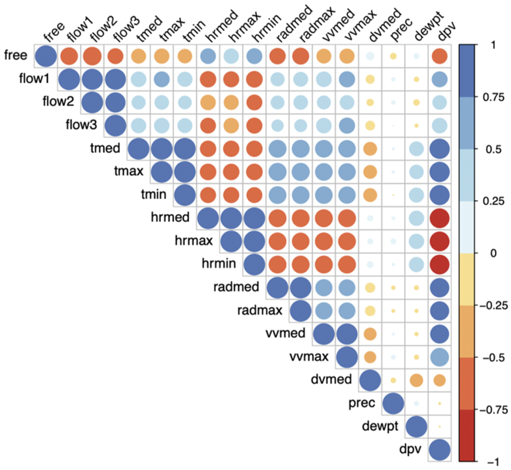
Figure 2: Correlation plot of all considered input variables
Regarding the mobility flows, we can see from Fig. 2 that the three of them have a negative correlation with the parking-space variable. However, flows ImA and ImB had a slightly higher negative correlation (−0.642, −0.719) than the flow for the area mC (−0.437) so we opted for just including the two former flows to the predictor. This difference in the coefficients makes sense as area mC is the one more distant to the target parking lots location (see Fig. 1). Hence, it associated latent mobility had a lower impact on the actual demand of the parking lots.
For the sake of clarity, Fig. 3 shows the two mobility flows selected from the analysis, ImA and ImB. Both flows are depicted along with the evolution of available parking spaces during the whole period of study.
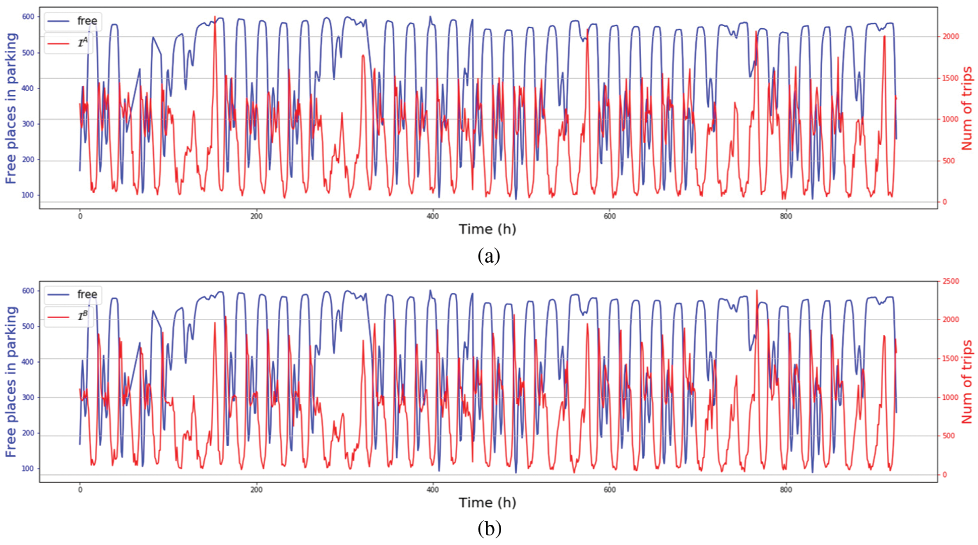
Figure 3: The two human mobility flows finally used for the prediction task along with number of available parking spaces during the period of study (a) Available parking spaces and the ImA flow during the period of study (b) Available parking spaces and the ImB flow during the period of study
Furthermore, there are many phenomena in which the past influences the present in the sense that they can be used to foretell what will happen. When such phenomena are represented as a time series, they are said to have an auto-regressive property. The correlation for univariate time series observations with previous time steps, called lags, is an autocorrelation. A plot of the autocorrelation of a time series by lag is called the AutoCorrelation Function (ACF). In this case, instead of correlation between two different variables, the autocorrelationat lag k is between two values of the same variable at times xi and xi+k. The previous formula is then transformed to the following,
Finally, partial autocorrelation is a summary of the relationship between an observation in a time series with observations at prior time steps with the relationships of intervening observations removed. The autocorrelation for an observation and some prior time step of itself is comprised of both the direct correlation and indirect correlations. These indirect correlations are a linear function of the correlation of the observation, with observations at intervening time steps.
Fig. 4 shows that parking spaces have a positive autocorrelation in the first 7 lags, reaches its maximum negative autocorrelation in lag 12 and then again the best positive correlation is present 24 h later. Regarding the partial autocorrelation, we see that there are many values statistically significant. From this we can conclude that the free parking presents an autorregresive behaviour and that including lagged values as inputs of the predictive models will likely imply a greater accuracy.
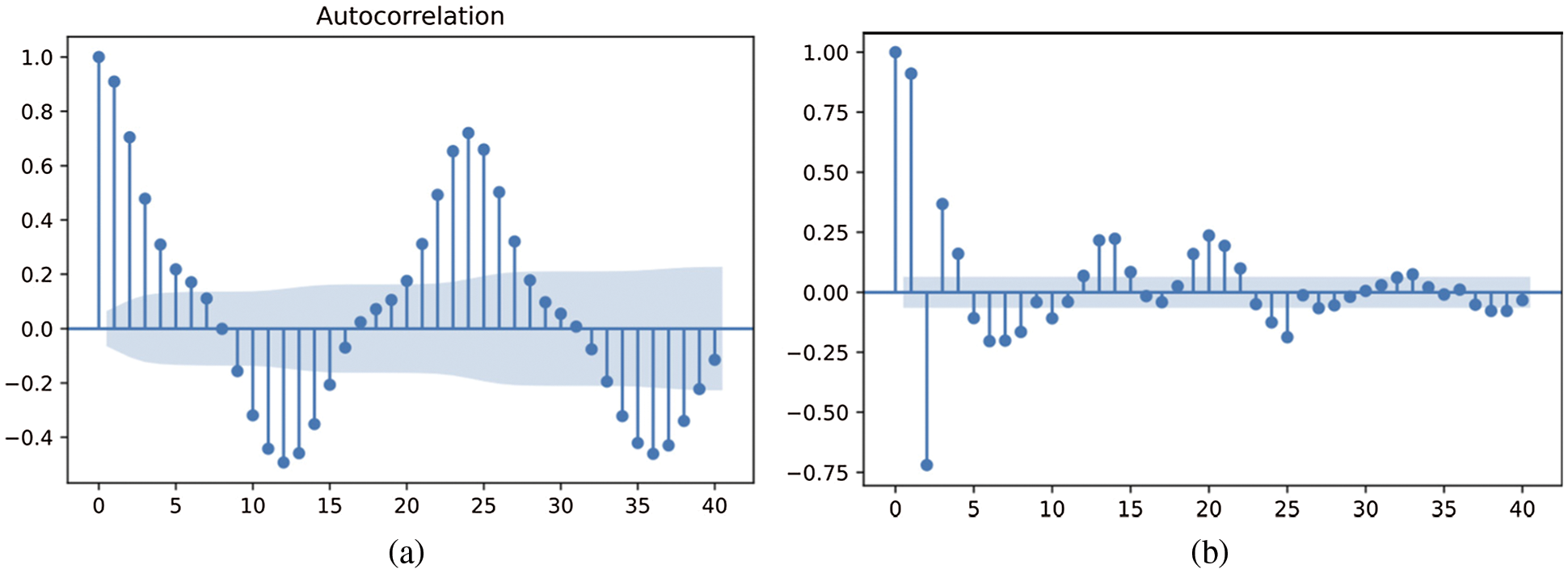
Figure 4: The visualization of the autocorrelation and partial autocorrelation of free parking spaces (a) Autocorrelation parking availability (b) Partial autocorrelation parking availability
4 Proposed Solution for Parking Space Prediction
In the light of the available datasources in the urban scenario and their suitability as independent variables for the prediction task at hand, we are now able to properly define a solution for parking space prediction based on them.
Our system takes as input three sources: historical data of available spaces in the target parking lots, the human mobility flows at low resolution and the weather conditions in the parkings’ surrounding areas.
The parking space prediction problem that we focus on can be formulated as follows:
Given the hour h ∈ ⟨0,…, 23⟩, the number of available parking spaces during the last hprev hours from the two target parking lots, Ph = (ph, ph−1,.., ph−hprev), the number of incoming trips of a set of MAs
4.2 Candidate Prediction Methods
Regarding the methods to develop the prediction task, we have considered three widely known neural networks, a Multi-Layer Perceptron (MLP), a Gated Recurrent Unit (GRU) and a Bidirectional Long-Short Term Memory (LSTM) network. A brief description of each of them is provided next.
This is one of the most popular and successful ANNs architectures that for a wide range of regression problems [42]. Its inner architecture basically comprises an input layer, one or more hidden layers and an output one where each layer is connected to another one by non-linear functions. Each layer comprises a set of neurons connected to all neurons of the next layer but not to each other. In computational terms, the output of a MLP layer be defined as h(W,b)(X) = φ(XW + b), where W is the connections’ weight matrix, X is the matrix with the input features, b is the vector with the bias terms and φ is the activation function.
Given the sequence nature of the two validated input sources of our approach, we have used a GRU model for the prediction task [43]. This is a foremost variant of Recurrent Neural Networks (RNN) able to learn short-term and long-term patterns in sequences of data. Unlike other RNNs, like LSTM, a GRU model has a slightly simpler structure which makes it faster to train [44].
Fig. 5a shows the general structure of a GRU network whereas Fig. 5b depicts the inner structure of a GRU cell. As we can see, a GRU model just follows the composition of a regular RNN. Concerning the structure of the cells, they make use of a gated mechanism to memorize long-term patterns in the target sequence. Thus, a cell receives as input the current input vector x(t) and the previous state vector h(t − 1). Then, the cell generates the associated output y(t) which is also the state vector h(t) of the next cell.
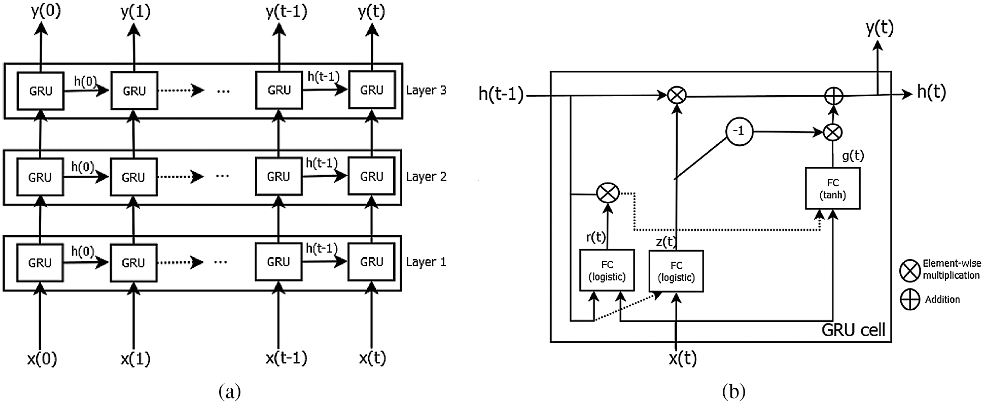
Figure 5: Illustrative architecture of the GRU model (a) A GRU model with three layers unrolled thought time (b) Gated structure of a GRU cell. FC stands for Fully Connected
More in detail, the cell comprises three different gates, the update z(t), the reset r(t) and the memory-content g(t). The computations of each gate are as follows,
where W{z,r,g} are the weight matrices for the input xt, U{z,r,g} are the weight matrices for the connections to the previous short-term state h(t − 1) and b{z,r,g} are the bias terms of each layer.
Last, we have evaluated a Long-Short Term Memory (LSTM) model. This is also a well-established RNN variant [45]. We have evaluated a bidirectional LSTM model [46]. Unlike a traditional LSTM network, a bidirectional approach allows the model not only to learn “causal” patterns by means of its past and present inputs but also to “look ahead” into the future. As Fig. 6a depicts, this is done by concatenating two RNNs one reading the input from left to right and the other from right to left. Then, the output of each cell is combined with its counterpart.
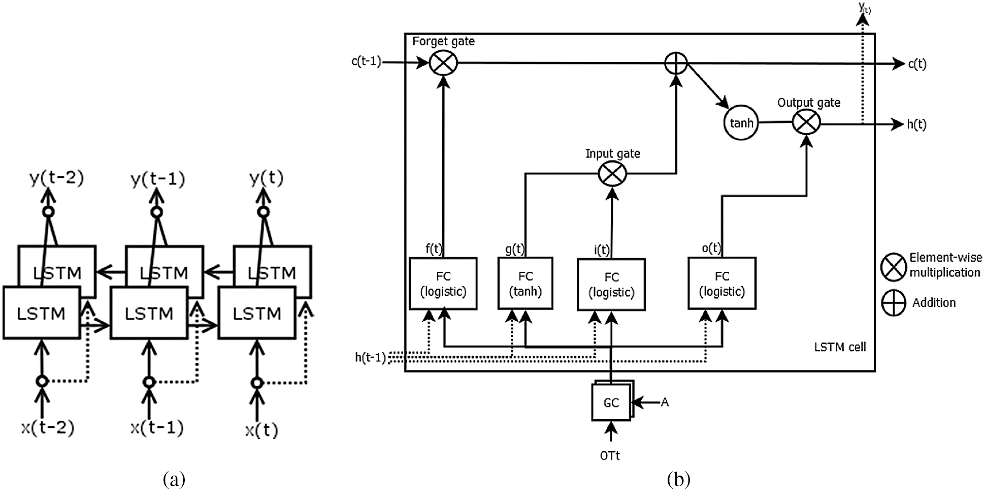
Figure 6: Illustrative architecture of the bidirectional LSTM model. (a) A bidirectional LSTM layer with six cells (b) Gated structure of a LSTM cell. FC stands for Fully Connected
The inner structure of a LSTM cell is depicted in Fig. 5b, where h(t−1) indicates the short-term state at time instant and x(t) is the current input vector at instant t. Concerning the cell outputs, y(t) is the predicted availability at instant t whereas c(t) is the long-term state that traverses the network from left to right. Focusing on the four inner gates of the cell that modulates the outputs of the model, they can be formulated as follows:
where x(t) is the parking availability at time instant t, W{f,i,o,g} are the weight matrices for this feature, U{f,i,o,g} are the weight matrices for the connections to the previous short-term state h(t−1) and b{f,i,o,g} are the bias terms of the four gates.
As we can see, the key difference between the GRU and the LSTM cell is that the former has three layers that are reset r(t), update z(t) and memory-content g(t) gates while the latter has four layers that are the input i(t), output o(t) and forget f(t) gates along with an output layer g(t). Thus, GRU is less complex than LSTM because it has a smaller number of gates.
The chosen period of analysis consisted of two ranges: 13th of July-31st of July and 29th of September-19th of October. We avoided August and September because in Murcia activities are reduced given the temperatures and holidays. Also, COVID-19 restrictions were more severe in those periods, so we decided to let them out of the analysis in order not to contaminate the sample. In the end, we considered 927 data points in roughly 2 months.
The raw parking data and the raw weather data are collected with more granularity than the mobility flows, that is 4 and 15 min respectively. However, we homogenised all data in hourly intervals, which was the mobility flows’ granularity. Given that we had to resample to a wider time frame, we used down-sampling and the aggregation function was the mean. After downsampling, due to failures in the communication system in the parking set, a 6% of the sample was missing. In order to impute the values, we used linear interpolation.
The performance of Deep Learning models and regression models is improved when scaling [47]. Scaling the inputs and outputs used in the training of the model is meaningful since small weights and errors in prediction values are used. Using unscaled inputs may slow or destabilize the learning process, while un-scaled target variables in regression problems may cause gradient explosions, leading to failure of the learning process. For that purpose, we have used Standardization (Z-score Normalization) in all our inputs. Feature standardization makes the values of each feature in the data have zero-mean (when subtracting the mean in the numerator) and unit variance. The formula is
All models had a training rate of 70 %, batch size 32 and learning factor 0.01, Mean Squared Error (MSE) as loss function and the Adam optimizer was used (α = 0.001, β1 = 0.9, β2 = 0.999, epsilon = 10−7). The hyperparameters of the models were selected using a grid search with Tab. 1 configuration. MLP used the ReLU activation function with 3 layers, 50 cells per layer and 50 epochs. GRU used the Hyberbolic tangent function for activation with 2 layers, 50–20 cells in each of them and 100 epochs. Finally, LSTM used the same activation function with 3 layers, 50–20–20 cells in each of them and 400 epochs.
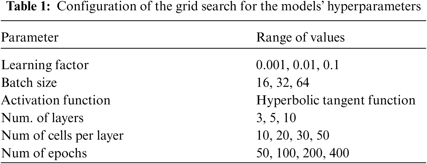
Fig. 7 shows the learning curves of the models with the provided configuration. As we can see, we avoid overfitting all models with the provided datasets.
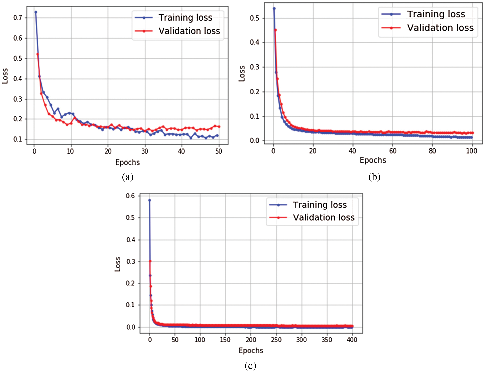
Figure 7: Learning curves of the three target models in the experiment. (a) MLP model (b) GRU model (c) Bi-LSTM model
Last, the number of parameters of these three models when they are fed with the incoming human flows, available parking spaces and weather conditions are 8801 in the case of the MLP, 13611 for the GRU model and 33321 for the bi-LSTM model.
4.4 Evaluation of the Approach
The MSE, Root Mean Squared Error (RMSE) and Mean Absolute Error (MAE) [48] are the most common metrics to measure accuracy for continuous variables. They are suitable for model comparisons because they express average model prediction error in the units of the variable of interest. Their definition is
Tab. 2 shows the metric values obtained by the models. This table also includes, as a baseline, a naive method that just returns the last value ph in each series as the predicted value p^h+T. Surprisingly, this type of straightforward mechanism is sometimes quite difficult to outperform.
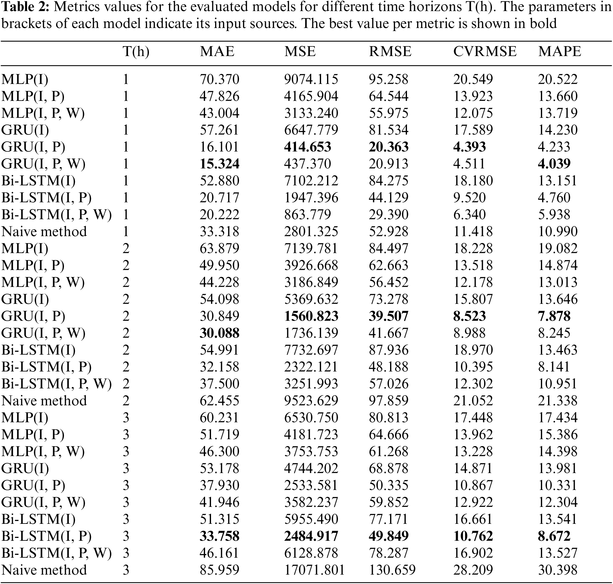
The table includes the results for 3 different hourly horizons (T): 1, 2 and 3 h ahead parking prediction. Obviously, a decrease in accuracy is observed the further we try to estimate, especially in the combinations (model and input) that provide better results. As was highlighted in bold in the table, GRU model is clearly better than the other alternatives in all cases. However, there are certain differences between metrics and scenarios when including or not the weather in the inputs.
In 1 h-ahead forecasting, when penalizing the points further away from the mean, the best combination of inputs includes previous parking observations and mobility flows: RMSE = 20.36 parking spaces and CVRMSE = 4.39%. However, when not penalizing it, the best combination includes also the weather information: MAE = 15.32 parking spaces and MAPE = 4.04%. The choice between the two depends on the objectives of parking spaces. We consider that if we are mistaken by 10 spaces should count more than just two times being mistaken by 5 spaces since precision is very important. Therefore, we would choose not to include the weather.
In 2 h-ahead and 3 h-ahead the better results are achieved when not considering the weather as input for all metrics, having a CVRMSE = 8.5% and CVRMSE = 10% respectively. For the 3 h-ahead scenario, the Bi-LSTM model achieved slightly better results than the GRU model. Nevertheless, it is important to remark that this improvement comes at the cost of using a much complex neural network as a bi-LSTM not only uses more complex cells than a GRU model but also its layers include extra connections (parameters) for the in-reverse flow of information as it was put forward in Sec. 4.2.3.
Fig. 8 shows the actual available spaces in the target parking lots in the test interval along with the predictions of the generated models for a time horizon T = 1 h. As we can see, the actual availability of the target parking lots follows a quite strong daily seasonal pattern. However, this figure also shows that only the GRU model was able to correctly predict the abnormal availability of the parking lots during the interval between the 80 and 120 h. This clearly shows a better matching between the prediction and the actual free parking when using GRU compared to MLP.
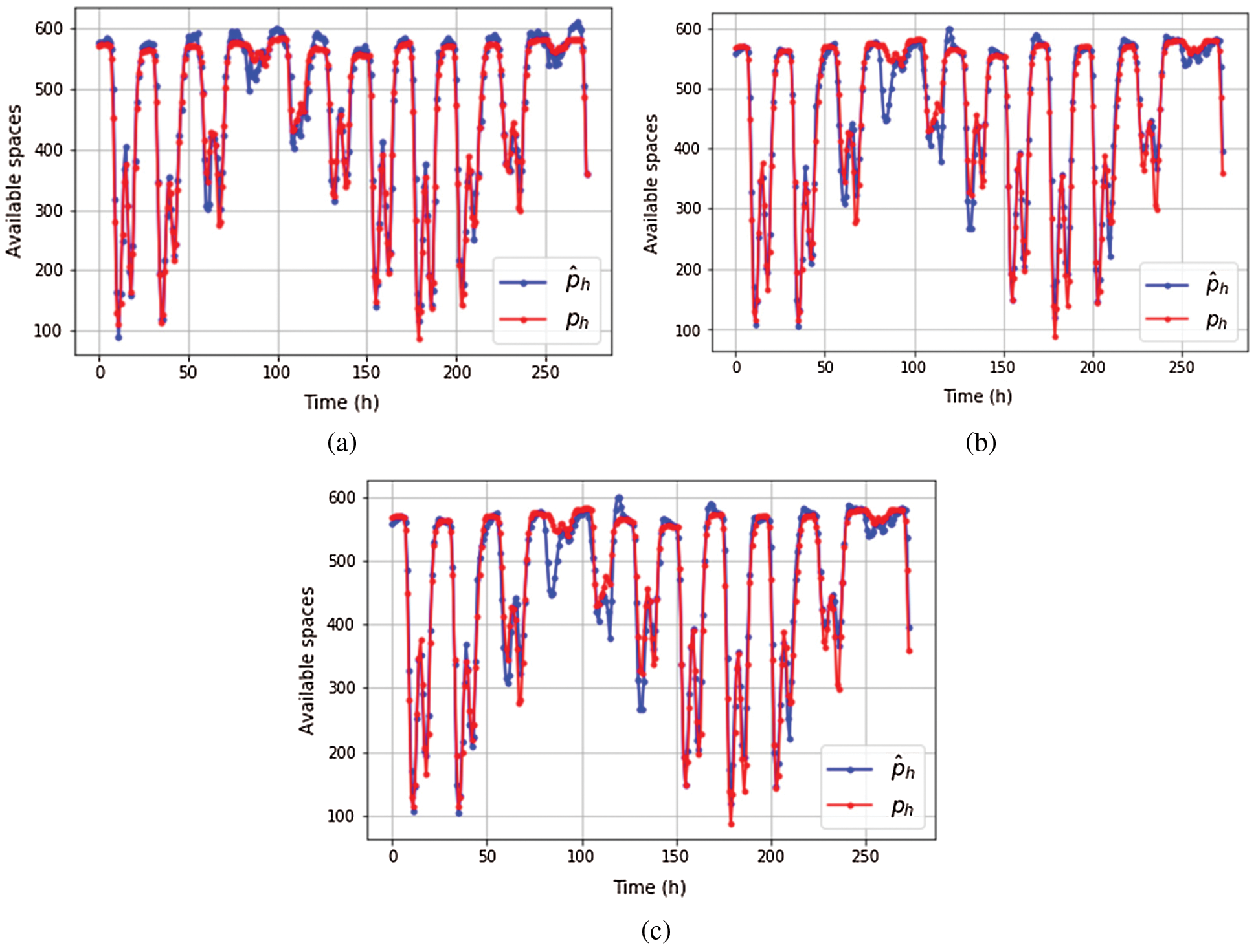
Figure 8: Time series of the available parking spaces
Finally, Tab. 3 shows a comparison between the results obtained by our solution and previous approaches in the literature for availability prediction in closed parking lots (Sec. 2.3).
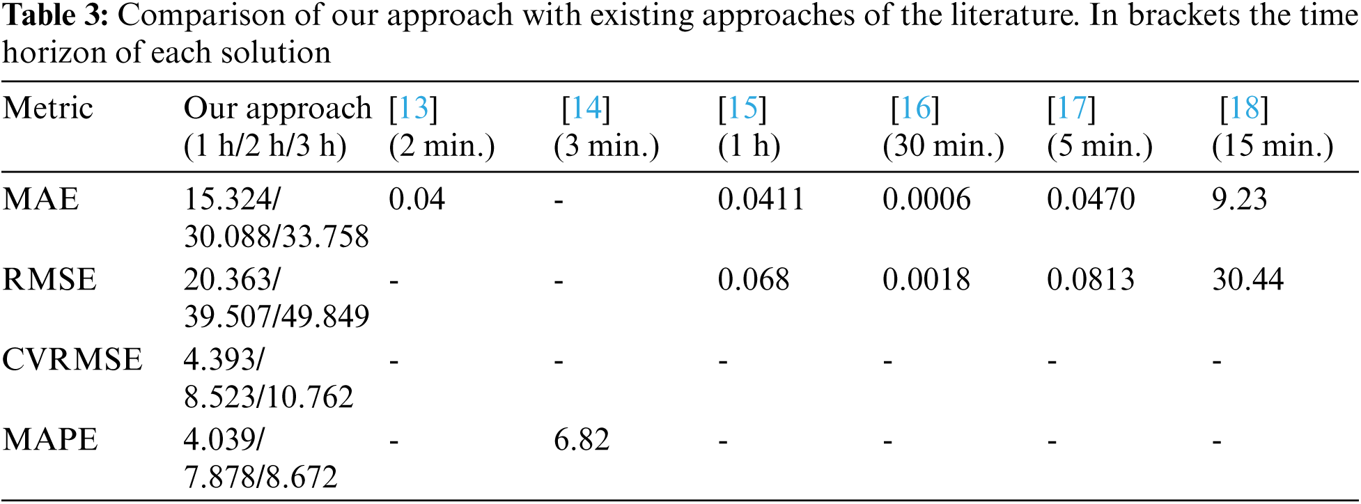
From this table, it is important to remark that results in [13–17] are given with respect the occupancy rate of the car parks. If we compare such values with the computed rate-based metrics of our approach (0.0233 MAE and 0.0311 RMSE for 1 h time horizon), we can see that our approach obtained slightly more accurate results. Furthermore, the time horizon is much larger than the baseline approaches as they range from a few minutes to 1 h. Regarding the proposal in [18], the absolute values of the metrics are also quite similar with a much larger time horizon.
All in all, results state that the usage of the human mobility dataset has clearly improved the accuracy of the predictor. However, such a dataset reflects all types of human displacements without considering the adopted means of transport. Since the parking lots are only used by motorized vehicles, the impact of using the SMT feed also reflects that the human mobility contained in this source is mainly defined by private-car trips. Consequently, this also confirms the fact that such vehicles are still the dominant means of transport for regular trips in most urban settlements.
The management of road traffic in large cities is one of the most challenging problems for authorities and operators. Since many urban traffic jams are caused by drivers searching for parking spaces, the accurate prediction of available spaces is an instrumental tool to enable efficient road-traffic policies.
However, most of the existing solutions generally assume that such contextual data is easily available through a large palette of location sensors. This limits the usability of current solutions because the access to location data in most real-world scenarios is restricted due to many regulations.
In this context, the present work proposes a novel mechanism for parking space prediction that leverages area-based human mobility data as the primary contextual source. The key goal was to evaluate whether such a coarse-grained mobility feed was useful to detect latent movement behaviors in particular locations within a city. To do so, we tested our approach in a real-world setting by making use of different ANNsto predict the available spaces of two downtown parking lots. Results have shown that enriching the models with the flows from the open dataset meaningfully improved their prediction accuracy.
In the future, with regards to research, our system can be used to feed fine-grained systems to improve their generalisation and also to study general parking patterns between cities to develop transfer the extracted knowledge between the similar ones using transfer learning. With regards to the development of new services, our parking availability prediction can be part of a system that includes route suggestions to drivers according to users’ preferences with regards to time, pollution, money, and availability to use other transport services in conjunction with their private car. Also, a new business model can emerge, such as the automatic, hourly, and renting of private parking spaces according to real-time needs.
Code availability: The source code of the project is available at https://github.com/fterroso/mobility_murcia_umu_ucam.
Funding Statement: This work has been sponsored by UMU-CAMPUS LIVING LAB EQC2019-006176-P funded by ERDF funds, by the European Commission through the H2020 PHOENIX (grant agreement 893079) and DEMETER (grant agreement 857202) EU Projects. It was also co-financed by the European Social Fund (ESF) and the Youth European Initiative (YEI) under the Spanish Seneca Foundation (CARM).
Conflicts of Interest: The authors declare that they have no conflicts of interest to report regarding the present study.
2https://www-03.ibm.com/press/us/en/pressrelease/35515.wss
3https://www.mitma.es/ministerio/covid-19/evolucion-movilidad-big-data/opendata-movilidad
4https://mapamurcia.inf.um.es/
1. D. Mage, G. Ozolins, P. Peterson, A. Webster, R. Orthofer et al., “Urban air pollution in megacities of the world,” Atmospheric Environment, vol. 30, no. 5, pp. 681–686, 1996. [Google Scholar]
2. V. Paidi, H. Fleyeh, J. Hakansson and R. G. Nyberg, “Smart parking sensors, technologies and applications for open parking lots: A review,” IET Intelligent Transport Systems, vol. 12, no. 8, pp. 735–741, 2018. [Google Scholar]
3. P. Wan-Joo, K. Byung-Sung, S. Dong-Eun, K. Dong-Suk and L. Kwae-Hi, “Parking space detection using ultrasonic sensor in parking assistance system,” in 2008 IEEE Intelligent Vehicles Symposium, Eindhoven, Netherlands, pp. 1039–1044, 2008. [Google Scholar]
4. F. Bock, S. Di Martino and A. Origlia, “Smart parking: Using a crowd of taxis to sense on-street parking space availability,” IEEE Transactions on Intelligent Transportation Systems, vol. 21, no. 2, pp. 496–508, 2020. [Google Scholar]
5. F. Shi, D. Wu, D. I. Arkhipov, Q. Liu, A. C. Regan et al., “Parkcrowd: Reliable crowdsensing for aggregation and dissemination of parking space information,” IEEE Transactions on Intelligent Transportation Systems, vol. 20, no. 11, pp. 4032–4044, 2019. [Google Scholar]
6. M. von Mörner, “Application of call detail records-chances and obstacles,” in World Conf. on Transport Research-WCTR 2016 Shanghai, Shanghai, China, pp. 2233–2241, 2016. [Google Scholar]
7. H. F. Chan, A. Skali and B. Torgler, “A global dataset of human mobility,” Tech. rep., Center for Research in Economics, Management and the Arts (CREMA), 2020. [Google Scholar]
8. G. Barlacchi, M. De Nadai, R. Larcher, A. Casella, C. Chitic et al., “A multi-source dataset of urban life in the city of Milan and the province of Trentino,” Scientific Data, vol. 2, no. 1, pp. 1–15, 2015. [Google Scholar]
9. S. Chang, E. Pierson, P. W. Koh, J. Gerardin, B. Redbird et al., “Mobility network models of covid-19 explain inequities and inform reopening,” Nature, vol. 189, no. 7840, pp. 82–87, 2020. [Google Scholar]
10. S. G. Kwak and J. H. Kim, “Central limit theorem: The cornerstone of modern statistics,” Korean Journal of Anesthesiology, vol. 70, no. 2, pp. 144–156, 2017. [Google Scholar]
11. Secretaría de Estado de Transportes, Movilidad y Agenda Urbana, “Análisis de la movilidad en España con tecnología Big Data durante el estado de alarma para la gestión de la crisis del COVID-19,” Tech. rep., Ministerio de Transportes, 2020. [Google Scholar]
12. M. Nilsson and S. von Corswant, “How certain Are You of getting a parking space?: A deep learning approach to parking availability prediction,” 2020. [Google Scholar]
13. S. Yang, W. Ma, X. Pi and S. Qian, “A deep learning approach to real-time parking occupancy prediction in transportation networks incorporating multiple spatio-temporal data sources,” Transportation Research Part C: Emerging Technologies, vol. 107, pp. 248–265, 2019. [Google Scholar]
14. W. Shao, Y. Zhang, B. Guo, K. Qin, J. Chan et al., “Parking availability prediction with long short-term memory model,” in 13th Int. Conf. on Green, Pervasive, and Cloud Computing, Springer International Publishing, Hangzhou, China, pp. 124–137, 2019. [Google Scholar]
15. S. L. Tilahun and G. Di Marzo-Serugendo, “Cooperative multiagent system for parking availability prediction based on time varying dynamic markov chains,” Journal of Advanced Transportation, vol. 2017, 14 pages, 2017. [Google Scholar]
16. J. Xiao, Y. Lou and J. Frisby, “How likely am I to find parking? – A practical model-based framework for predicting parking availability,” Transportation Research Part B: Methodological, vol. 112, pp. 19–39, 2018. [Google Scholar]
17. L. Xiangdong, C. Yuefeng, C. Gang and X. Zengwei, “Prediction of short- term available parking space using LSTM model,” in 2019 14th Int. Conf. on Computer Science Education (ICCSE), Toronto, Canada, pp. 631–635, 2019. [Google Scholar]
18. G. Ali, T. Ali, M. Irfan, U. Draz, M. Sohail et al., “IoT based smart parking system using deep long short memory network,” Electronics, vol. 9, no. 10, 2020. [Google Scholar]
19. S. C. Koumetio Tekouabou, E. A. Abdellaoui Alaoui, W. Cherif and H. Silkan, “Improving parking availability prediction in smart cities with IoT and ensemble-based model,” Journal of King Saud University–Computer and Information Sciences, in press, 2020. [Google Scholar]
20. W. Shao, S. Zhao, Z. Zhang, S. Wan, M. S. Rahaman et al., “FADACS: A few-shot adversarial domain adaptation architecture for context-aware parking availability sensing,” in 2021 IEEE Int. Conf. on Pervasive Computing and Communications (PerCom), Kassel, Germany, pp. 1–10, 2021. [Google Scholar]
21. W. Zhang, H. Liu, Y. Liu, J. Zhou and H. Xiong, “Semi-supervised hierarchical recurrent graph neural network for city-wide parking availability prediction,” in AAAI Conf. on Artificial Intelligence 2020, New York, USA, pp. 1186–1193, 2020. [Google Scholar]
22. O. Abdulkader, A. M. Bamhdi, V. Thayananthan, K. Jambi and M. Alrasheedi, “A novel and secure smart parking management system (SPMS) based on integration of WSN, RFID, and IoT,” in 2018 15th Learning and Technology Conf. (L&T), Jeddah, Saudi Arabia, pp. 102–106, 2018. [Google Scholar]
23. E. I. Vlahogianni, K. Kepaptsoglou, V. Tsetsos and M. G. Karlaftis, “A real-time parking prediction system for smart cities,” Journal of Intelligent Transportation Systems, vol. 20, no. 2, pp. 192–204, 2016. [Google Scholar]
24. R. F. Pozo, A. B. R. González, M. R. Wilby, J. J. V. Díaz and M. V. Matesanz, “Prediction of On-Street Parking Level of Service Based on Random Undersampling Decision Trees,” IEEE Transactions on Intelligent Transportation Systems, in press, 2021. [Google Scholar]
25. M. Barraco, N. Bicocchi, M. Mamei and F. Zambonelli, “Forecasting parking lots availability: Analysis from a real-world deployment,” in 2021 IEEE Int. Conf. on Pervasive Computing and Communications Workshops and other Affiliated Events, Kassel, Germany, pp. 299–304, 2021. [Google Scholar]
26. H. Bura, N. Lin, N. Kumar, S. Malekar, S. Nagaraj et al., “An edge based smart parking solution using camera networks and deep learning,” in 2018 IEEE Int. Conf. on Cognitive Computing (ICCC), IEEE, San Francisco, USA, pp. 17–24, 2018. [Google Scholar]
27. F. Terroso-Saenz, A. Muñoz and F. Arcas, “Land-use dynamic discovery based on heterogeneous mobility sources,” International Journal of Intelligent Systems, vol. 36, no. 1, pp. 478–525, 2021. [Google Scholar]
28. F. Terroso-Sáenz, J. Cuenca-Jara, A. González-Vidal and A. F. Skarmeta, “Human mobility prediction based on social media with complex event processing,” International Journal of Distributed Sensor Networks, vol. 12, no. 9, 2016. [Google Scholar]
29. J. Cuenca-Jara, F. Terroso-Saenz, M. Valdes-Vela, A. Gonzalez-Vidal and A. F. Skarmeta, “Human mobility analysis based on social media and fuzzy clustering,” in 2017 IEEE Global Internet of Things Summit (GIoTS), Geneva, Switzerland, pp. 1–6, 2017. [Google Scholar]
30. F. M. Awan, Y. Saleem, R. Minerva and N. Crespi, “A comparative analysis of machine/deep learning models for parking space availability prediction,” MDPI Sensors Journal, vol. 20, no. 1, 2020. [Google Scholar]
31. R. Jozefowicz, W. Zaremba and I. Sutskever, “An empirical exploration of recurrent network architectures,” in 32nd Int. Conf. on Machine Learning. Proc. of Machine Learning Research (PMLR), vol. 37, Lille, France, pp. 2342–2350, 2015. [Google Scholar]
32. J. Arjona, M. Linares, J. Casanovas-Garcia and J. J. Vázquez, “Improving parking availability information using deep learning techniques,” Transportation Research Procedia, vol. 47, pp. 385–392, 2020. [Google Scholar]
33. W. Zhang, H. Liu, Y. Liu, J. Zhou and H. Xiong, “Semi-supervised hierarchical recurrent graph neural network for city-wide parking availability prediction,” in Proc. of the AAAI Conf. on Artificial Intelligence, New York City, USA, vol. 34, no. 1, pp. 1186–1193, 2020. [Google Scholar]
34. J. Guo, S. Zhang, J. Zhu and R. Ni, “Measuring the Gap between the maximum predictability and prediction accuracy of human mobility,” IEEE Access, vol. 8, pp. 131859–131869, 2020. [Google Scholar]
35. S. Dokuz, “Fast and efficient discovery of key bike stations in bike sharing systems big datasets,” Expert Systems with Applications, vol. 172, pp. 114659, 2021. [Google Scholar]
36. E. Toch, B. Lerner, E. Ben-Zion and I. Ben-Gal, “Analyzing large-scale human mobility data: A survey of machine learning methods and applications,” Knowledge and Information Systems, vol. 58, no. 3, pp. 501–523, 2019. [Google Scholar]
37. F. Terroso-Sáenz and A. Muñoz, “Nation-wide human mobility prediction based on graph neural networks,” Applied Intelligence, pp. 858–863, in press, 2021. [Google Scholar]
38. A. Gonzalez-Vidal, F. Jimenez and A. F. Gomez-Skarmeta, “A methodology for energy multivariate time series forecasting in smart buildings based on feature selection,” Energy and Buildings, Elsevier, vol. 196, pp. 71–82, 2019. [Google Scholar]
39. A. Gonzalez-Vidal, F. Jimenez and A. F. Gomez-Skarmeta, “A methodology for energy multivariate time series forecasting in smart buildings based on feature selection,” Energy and Buildings, vol. 196, pp. 71–82, 2019. [Google Scholar]
40. A. Gonzalez-Vidal, T. Alcañiz, T. Iggena, E. B. Ilyas and A. F. Skarmeta, “Domain agnostic quality of information metrics in IoT-based smart environments,” in Intelligent Environments 2020: Workshop Proc. of the 16th Int. Conf. on Intelligent Environments, Madrid, Spain, vol. 28, pp. 343–352, 2020. [Google Scholar]
41. V. S. Brum-Bastos, J. A. Long and U. Demásar, “Weather effects on human mobility: A study using multi-channel sequence analysis,” Computers, Environment and Urban Systems, vol. 71, pp. 131–152, 2018. [Google Scholar]
42. O. I. Abiodun, A. Jantan, A. E. Omolara, K. V. Dada, N. A. Mohamed et al., “State-of-the-art in artificial neural network applications: A survey,” Heliyon, vol. 4, no. 11, pp. 1–41, 2018. [Google Scholar]
43. K. Cho, B. van Merrienboer, C. Gulcehre, F. Bougares, H. Schwenk. et al., “Learning phrase representations using rnn encoder-decoder for statistical machine translation,” in Conf. on Empirical Methods in Natural Language Processing (EMNLP 2014), Doha, Qatar, pp. 1724–1734, 2014. [Google Scholar]
44. J. Chung, C. Gulcehre, K. Cho and Y. Bengio, “Empirical evaluation of gated recurrent neural networks on sequence modeling,” in 28th Conf. on Neural Information Processing Systems 2014 Workshop on Deep Learning, Quebec, Canada, 2014. [Google Scholar]
45. S. Hochreiter and J. Schmidhuber, “Long short-term memory,” Neural Computation, vol. 9, no. 8, pp. 1735–1780, 1997. [Google Scholar]
46. M. Schuster and K. K. Paliwal, “Bidirectional recurrent neural networks,” IEEE Transactions on Signal Processing, vol. 45, no. 11, pp. 2673–2681, 1997. [Google Scholar]
47. J. Grus, “Data science from scratch: First principles with python,” USA: O'Reilly Media, 2019. [Google Scholar]
48. J. Willmott and K. Matsuura, “Advantages of the mean absolute error (MAE) over the root mean square error (RMSE) in assessing average model performance,” Climate Research, vol. 30, no. 1, pp. 79–82, 2015. [Google Scholar]
49. E. I. Vlahogianni, K. Kepaptsoglou, V. Tsetsos and M. G. Karlaftis, “A real- time parking prediction system for smart cities,” Journal of Intelligent Transportation Systems, vol. 20, no. 2, pp. 192–204, 2016. [Google Scholar]
 | This work is licensed under a Creative Commons Attribution 4.0 International License, which permits unrestricted use, distribution, and reproduction in any medium, provided the original work is properly cited. |