DOI:10.32604/cmc.2022.023003
| Computers, Materials & Continua DOI:10.32604/cmc.2022.023003 | |
| Article |
Edge Metric Dimension of Honeycomb and Hexagonal Networks for IoT
1Department of Computer Science, College of Computing and Informatics, University of Sharjah, Sharjah, 27272, UAE
2Department of Mathematics, College of Sciences, University of Sharjah, Sharjah, 27272, UAE
3Artificial Intelligence Lab, Department of Computer Engineering, Gachon University, Seongnam, 13557, Korea
*Corresponding Author: Taegkeun Whangbo. Email: tkwhangbo@gachon.ac.kr
Received: 25 August 2021; Accepted: 27 September 2021
Abstract: Wireless Sensor Network (WSN) is considered to be one of the fundamental technologies employed in the Internet of things (IoT); hence, enabling diverse applications for carrying out real-time observations. Robot navigation in such networks was the main motivation for the introduction of the concept of landmarks. A robot can identify its own location by sending signals to obtain the distances between itself and the landmarks. Considering networks to be a type of graph, this concept was redefined as metric dimension of a graph which is the minimum number of nodes needed to identify all the nodes of the graph. This idea was extended to the concept of edge metric dimension of a graph G, which is the minimum number of nodes needed in a graph to uniquely identify each edge of the network. Regular plane networks can be easily constructed by repeating regular polygons. This design is of extreme importance as it yields high overall performance; hence, it can be used in various networking and IoT domains. The honeycomb and the hexagonal networks are two such popular mesh-derived parallel networks. In this paper, it is proved that the minimum landmarks required for the honeycomb network HC(n), and the hexagonal network HX(n) are 3 and 6 respectively. The bounds for the landmarks required for the hex-derived network HDN1(n) are also proposed.
Keywords: Edge metric dimension; internet of things; wireless sensor network; honeycomb network; hexagonal network; hex-derived networks
Honeycomb and Hexagonal networks [1] have been widely studied in various research domains, such as wireless sensor networks, wireless networks [2–6] and cellular networks, in order to study and analyze various issues like routing, [7–9] location management and target tracking [10–12], energy conservation [13–15], and interference estimation [16]. These networks and application domains are applicable to the IoT as well [17–24]. The concept of metric basis and metric dimension for the purpose of robot navigation within a graph-structured framework was initially studied in [25]. Recently, the concept of robots and drones have also been proposed in such network structures for various application reasons [26]. For example, drones/robots might be used in wireless sensor networks to gather samples for maintenance inspection or regular data collection acting as a mobile sink. Similarly, they can also be used to recharge the batteries of dying sensors on-the-fly.
Suppose an IoT scenario where a robot/drone is dropped somewhere unknown in a network and can move from node to node. Some vertices in the graph behave as landmarks, and the robot can measure its distance in the graph to any landmark. The objective of this work is to find the fewest number of landmarks so that the robot can determine its current node by only using the distances to the landmarks. While dealing with navigation problems, networks are referred to as graphs G, the elements of the metric basis as landmarks, the minimum size of the metric basis as metric dimension dim(G) and the remaining vertices as nodes and identified the metric dimension of certain simple categories of graphs. The concept of metric basis also yielded significant applications in chemistry, drug design, image processing and combinatorial optimization [27].
But what if the robot takes edges into consideration while calculating distance to any landmark. Can the robot still measure its distance in the graph to any landmark such that the landmarks distinguish the edges instead of vertices? A metric basis S of a connected graph G uniquely identifies all the nodes of G by means of distance vectors. One could think that the edges of the graph are also identified by S with respect to the distances to S. However, this does not happen. For instance, Fig. 1 shows an example of a graph, where no metric basis uniquely recognizes all the edges of the graph.
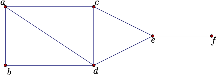
Figure 1: The simple graph G
It can be observed that the graph G of Fig. 1 satisfies that dim(G) = 2. But for each one of the metric bases, there exist at least a pair of edges which is not distinguished by the corresponding metric basis as shown in Tab. 1. For the metric basis {a, b} the edges ac and ad are equidistant from it while for the metric basic {c, d}, the edges ad and bd are equidistant and so on. In this sense, a natural question is: Are there some sets of vertices/nodes which uniquely identify all the edges of a graph? To answer this, a new parameter was recently introduced in which the question is to whether there are some sets of nodes which can uniquely identify all the edges of a graph [28].
Let G = (V, E) be a connected graph. Let x ∈ V be a node and e = uv ∈ E be an edge, then the distance between the node x and the edge e is defined as dG (e, x) = min {dG (u, x), dG (v, x)}. A node x distinguishes any two edges e, f if dG (x, e) ≠ dG (x, f). A set S ⊂ V is an edge metric generator (EMG) for G if for any two distinct edges e1 and e2, there exists at least one node v ∈ S such that the distances dG (e1, v) and dG (e2, v) are different. An EMG with the smallest size is referred to as an edge metric basis (EMB) for G, and its size is an edge metric dimension (EMD), which is denoted by edim(G). Another useful approach for an EMG is as follows. Given an ordered set of nodes S = (s1, s2,…, sd ) of a connected graph G, for any edge e in G, the d-vector (ordered d-tuple) is referred to as r(e|S ) = (dG (e, s1), dG (e, s2),…, dG (e, sd )) as the edge metric representation of e with respect to S. In this sense, S is an EMG for G if and only if for every pair of different edges e1, e2 of G, r(e1|S ) ≠ r(e2|S ) [29].
In [29], it was proved that the edim(G) = 1 if and only if it is a path. They also proved that paths Pn, cycles Cn and complete graphs Kn are families of graphs for whom dim(G) = edim(G).
The determination of EMD is NP hard problem. Hence, one has to consider particular classes of graphs. In [30,31], the author characterized the graphs for which edim(G) = n − 1. The EMD of some graph products was computed in terms of the graphs of the products [32].
In this paper the following have been proved:
• The EMD of Honeycomb networks is 3.
• The EMD of Hexagonal networks is 6.
• The upper bound of two extensions of these networks called the Hex derived networks is proposed.
The rest of the manuscript is organized as follows. Section 2 provides the background of honeycomb and hexagonal networks along with their applications plus the related research in this domain. In Section 3, the edge metric dimension of the honeycomb and hexagonal networks are discussed where the resolving set for the HDN1(n) network is presented. The paper is concluded in the Section 4 while highlighting the limitations and future direction of the proposed work.
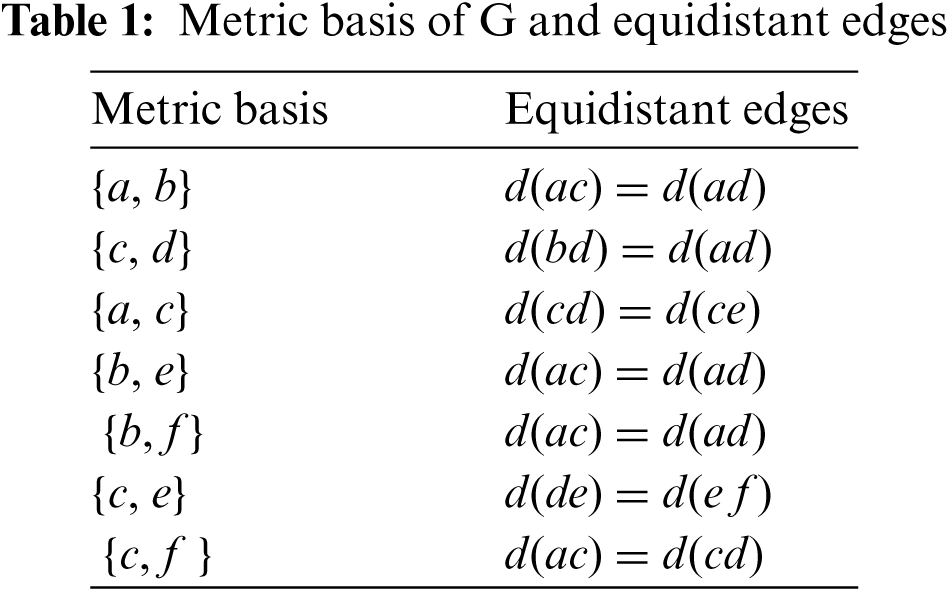
The honeycomb networks are built by recursively using the hexagonal tessellation [33]. The honeycomb network can be easily built from simple hexagons in various ways. HC(1) is just a simple hexagon. Adding one hexagon to each edge of this hexagon gives us HC(2). Similarly, HC(n) can be obtained in the same manner. The network cost, defined as the product of degree and diameter, is better for honeycomb networks than for the two other families based on square (mesh-connected computers and tori) and triangular (hexagonal meshes and tori) tessellations. Honeycomb networks provide simple and optimal routing, broadcasting, and semigroup computation algorithm. Honeycomb networks have major applications in mobile base stations, sensor networks, image processing, and computer graphics. The topological properties of honeycomb networks, their routing as well as torus honeycomb networks have been studied in [33].
On the other hand, the hexagonal network which was introduced in [34] is made of a minimum of six triangles and denoted by HX(2) whereas HX(1) does not exist. HX(3) comes from adding a series of triangles around HX(2). This pattern can be extended to HX(n). It is easy to see that n is the number of nodes on any one of the outermost edges of the hexagonal network, see Fig. 2.
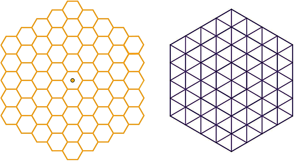
Figure 2: Honeycomb HC(4) and hexagonal HX(5) networks
Hexagonal networks also have many applications in wireless communication systems, where the cellular concept plays an important role in solving the problem of spectral congestion and capacity. Hence, the hexagonal concept of model coverage plays an important role in such cellular network communications.
Multiprocessor interconnection networks are often required to connect thousands of homogeneously replicated processor-memory pairs, each of which is called a processing node. Instead of using a shared memory, all synchronization and communication between processing nodes for program execution is often done via message passing. Design and use of multiprocessor interconnection networks have recently drawn considerable attention due to the availability of inexpensive, powerful microprocessors and memory chips [34,35]. Regular plane tessellations can be easily constructed by repeating regular polygons. This design is of extreme importance for direct interconnection networks as it yields high overall performance.
A lot of research followed this and a host of generators, such as [36,37], were introduced. However, these generators primarily focused on the differentiation of the nodes. The idea was that a network in which a metric generator can distinguish the vertices behaves like an accurate surveillance activated network. But, if there is an intruder which accesses the network not through its vertices, but by using some connections between them (edges), then such intruder could not be identified, and in this sense, the surveillance fails in its commitment and some extra property is required in the network to be used effectively for this purpose [38]. The honeycomb and hexagonal networks along with the security are studied in [39]. Hence, such limitation can cause a major disadvantage from the application point of view. It is this shortcoming, that motivated the authors to explore a unique edge metric generator for this family of networks.
3 Result Discussions and Analysis
In this section, the EMD of the Honeycomb and hexagonal networks will be computed. The bounds for one of the hex derived networks will also be proposed. It is interesting to find that the EMD of honeycomb network and the hexagonal network are constant. For the hex-derived networks, it still needs to be seen whether an exact value for the EMD can be obtained or not.
3.1 Edge Metric Dimension of the Honeycomb Network
In this subsection, the EMD will be computed for the Honeycomb network HC(n), It is interesting to note that the EMD is the same as the metric dimension of the honeycomb network. This will provide a partial answer to the question about the families of graphs for which the EMD and the usual metric dimension are same. In order to prove the EMD for the honeycomb network, first the paths for this network are defined. Let αPi, βPj and γPk be paths defining HC(n) such that 0 ≤ i, j, k ≤ 2n − 1 as shown in the Fig. 3. It is easy to see that each edge is the intersection of exactly two different paths.
Figure 3: Paths in honeycomb network-HC(4)
Theorem 1. Let HC(n) be the honeycomb network. Then edim(HC(n)) = 3.
Proof: This proof consists of two parts, where the first part is divided into three cases depending upon the paths, and the second part is divided into two cases. The first part of the proof is of forward inequality followed by proof of backward inequality thus leading to the equality itself. Since the honeycomb network is built recursively using the hexagonal tessellation, its properties exhibit symmetry across various dimensions. It is to explain these properties, that the proof is further divided into Cases, sometimes followed by sub-cases to further explain the unique cases underlying a particular pattern.
It will be proved that R = {α, β, γ} is a resolving set for HC(n). As one can see from Fig. 3, that HC(n) network consists of three types of edges with respect to each node in R. For simplicity, three types of edges with respect to α will be taken. The case of the edges with respect to the other nodes of R can be resolved in a similar manner. Let e1 and e2 be any two edges of HC(n). The following cases may ensue, depending on the types of edges.
Case 1: If both edges e1 and e2 belong to the same path αPi for some i, then they will be distinguished by α itself.
Case 2: If both edges e1 and e2 are parallel such that they lie between two consecutive paths αPi and αPi + 1 for some i, that is e1 and e2 does not completely lie on any of these two consecutive paths, then again, they will be distinguished by α.
Case 3: If e1 and e2 lie on two different paths αPi and αPj such that i ≠ j, then all such pair of edges e1 and e2 will be automatically distinguished by α except the pair of edges for whom d(e1, α) = d(e2, α). In this situation, two possibilities may arise, i.e., : Subcase 3a: If e1, e2 ∈ βPk for some k, then we are in Case 1 for the node β. Subcase 3b: If e1, e2 ∉ βPk for some k, then this happened only if e1 ∈ βP2k and e2 ∈ βPl + 1 for some k and l, then it is easy to see that d(e1, γ) < d(e2, γ) and both edges will be distinguished by γ. Hence, the edim(HC(n)) ≤ 3.
Conversely, it can be proved that the edim(HC(n)) ≥ 3. On the contrary, suppose that there is a resolving set of cardinality two, say S = {a, b} ∈ V(HC(n)). Since each node of HC(n) lies on some paths of α, β, γ, let us consider all the nodes lying on the paths indexed by γ. So, if there exits i and j such that a ∈ γPi and b ∈ γPj, then the following two cases are to be considered:
Case 1: If i = j, it means that both the nodes of S lie on a path γPi of even length l = 2q. If the distance between them is denoted by d(a, b) = m. then two cases may arise depending upon m.
Subcase 1a: If m < l, then there will exist two edges e1 and e2 incident to one of the nodes of S say a, such that one of the edges lies on the path γPi and the other does not. It is easy to see that d(e1 | S) = d(e2 | S) = (0, m).
Subcase 1b: If m = l, such that i = j ≠ n and a, b ∈ γPi, then there exists at least two edges e1 and e2 in γPi+1 and γPi − 1 such that d(e1 | S ) = d(e2 | S ) = (3, m - 2), a contradiction. If i = j = n and a, b ∈ γPn, then again there exists two edges e1 and e2 on γP3 such that d(e1 | S) = d(e2 | S) = (m + 1, m + 1), a contradiction.
Case 2: For i ≠ j, let a ∈ γPi and b ∈ γPj such that they also lie on αPr or βPs. Then we will be in Case 1 for α or β. If a ∈ γPi and b ∈ γPj such that they do not lie on αPr or βPs, then the following possibilities may ensue:
• If d(a, b) > 3, then there exists at least two edges e1 and e2 with the following properties: e1 and e2 are incident on a node of the shortest path between a and b, and one of the edges say e1 lies on the shortest path. Hence, d(a, e1) = d(a, e2) = 2 and d(e1 | S ) = d(e2 | S).
• If d(a, b) = 3, and a and b lie on two deferent hexagons, then one can find two edges e1 and e2 such that d(e1 | S) = d(e2 | S) = (0, 3).
• If d(a, b) = 3, and a and b lie on the same hexagon, then one can find two edges e1 and e2 such that d(e1 | S) = d(e2 | S) = (0, 2).
• If d(a, b) = 2, then one can find two edges e1 and e2 such that d(e1 | S) = d(e2 | S) = (0, 2).
• If d(a, b) = 1, then there exists two edges e1 and e2 such that d(e1 | S) = d(e2 | S) = (0, 1). Hence, the edim(HC(n)) > 3 and the proof is finished.
3.2 Edge Metric Dimension of the Hexagonal Network
In order to prove this, the concept of the co-ordinate system of the hexagonal network is presented as adapted by Nocetti et al. [39]. He introduced the three axes, X, Y and Z at an angle of 120 along the sides of any triangle within a hexagonal network as shown in the Fig. 4. In this section, the EMD for the hexagonal network HX(n) will be computed. It is interesting to note that the EMD is larger than the metric dimension of the hexagonal network. This will once again provide a partial answer to the question raised in [40] about the classification of families for which the EMD is larger than the usual metric dimension.
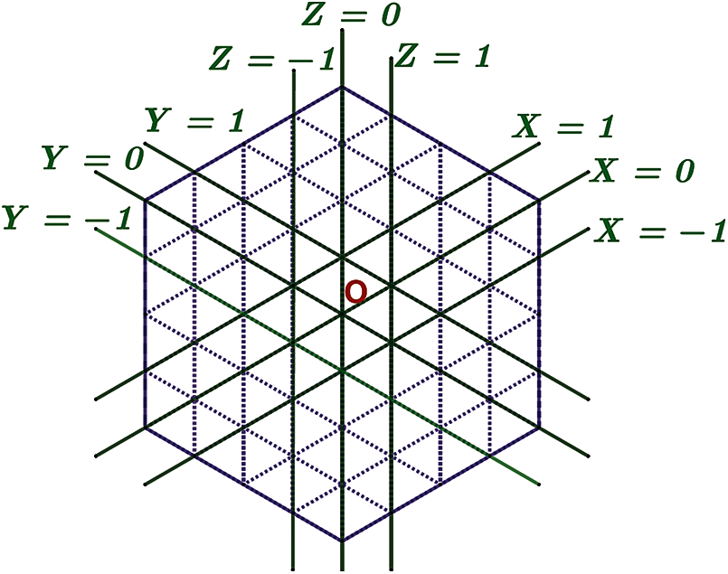
Figure 4: Coordinate system of hexagonal network-HX(5)
The concept of edge neighborhood of a node and state some properties of the same are introduced now. For any node v ∈ V(HX(n)) and e ∈ E(HX(n)), the edge neighborhood of a node v is defined as E Np(v) = {e | d(e, v) = p} where 0 ≤ p ≤ 2n − 2. For the convenience of describing the edges, the lines parallel to X-axis are referred to as X- lines and follow the same concept for defining Y- lines and Z- lines. Furthermore, a segment of any X, Y or Z line is referred to as SX, SY and SZ respectively as shown in the Fig. 4. The central node is labeled by o and the six corner nodes of the outer most hexagon as {α, β, γ, θ, σ, ψ} as shown in the Fig. 5.
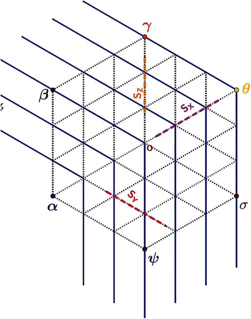
Figure 5: Neighborhoods of hexagonal network-HX(4)
Theorem 2. Let HX(n) be a hexagonal network. Then the edim(HX(n)) = 6
Proof. We will prove that R = {α, β, γ, θ, σ, ψ} is a resolving set for HX(n).
In order to proof that R = {α, β, γ, θ, σ, ψ} is a resolving set for G, the network is divided into 6 triangles namely Δαoψ, Δβoα, Δγoβ, Δθoγ, Δσoθ and Δψoσ.
The proof is presented in two steps. In the first step, it is proved that if e1 and e2 are two edges such that e1 and e2 belong to two different triangles, then they are distinguished by one of the nodes in R. In the second step, it is further proved that if e1 and e2 are two edges belonging to the same triangle, then once again they are distinguished by some node in R.
Case 1: Let e1 and e2 by two edges belongs to two different triangles. There are two subcases to consider depending upon the types of triangles.
Subcase 1a: Let e1 and e2 belong to two non-adjacent triangles. For simplicity let us take the two triangles Δαoψ and Δθoγ such that e1 ∈ Δαoψ and e2 ∈ Δθoγ. Then e1 ∈ E Np(α) such that 0 ≤ p ≤ n − 1 and e2 ∈ E Np(α) such that n − 1 ≤ p ≤ 2n − 2. Hence, at all times e1 and e2 will be distinguished by α ∈ R except when p = n − 1. In such a case, it is easy to see that e1 and e2 will be clearly distinguished by ψ.
Subcase 1b: Let e1 and e2 belong to two adjacent triangles. If e1 and e2 lie on the shared side of the two adjacent triangles, then they will fall under the restrictions of Case 2 discussed below. However, if the edges e1 and e2 are chosen such that e1 ∈ Δαoψ and e2 ∈ Δψoσ such that they do not lie on the shared side then it is observed that e1 ∈ E Np(α) such that 0 ≤ p ≤ n − 1 and e2 ∈ E Np(α) such that n − 1 ≤ p ≤ 2n − 3. Hence, e1 and e2 will be distinguished by α ∈ R except when p = n − 1. In such a case, it is easy to see that e1 and e2 will be clearly distinguished by σ. Symmetry leads to similar reasoning for the cases of any pair of edges belonging to any pair of triangles in the network.
Case 2: Let the two edges e1 and e2 belong to the same triangle, say Δψoσ. See Fig. 5. In this case, the following is observed:
Subcase 2a: If the two edges e1 and e2 lie on the same segment of one of the co-ordinate axes, say SZ of the Z- axis. Then it is easy to see that the two edges e1 and e2 are distinguished by ψ and γ. Similarly, if the edges belonged to SX or SY, then they will be distinguished by α and θ or β and σ respectively.
Subcase 2b: If two edges e1 and e2 are parallel to each other and lie on the segments of one of the axes, say SXi and SXj for i ≠ j. Then it is clear to note that there exists distinct indices p and q such that e1 ∈ E Np(β) and e2 ∈ E Nq(β) and hence the edges are distinguished by β. Similar observations will be observed if the edges belonged to SY or SZ.
Subcase 2c: If the two edges e1 and e2 lie on segments of two different axes, then the following two possibilities arise:
a)If two edges are incident on a node, for simplicity, it can be assumed that e1 = bd ∈ SZi for some i, then the following two possibilities arise:
• If e2 = ab ∈ SXj for some j, then e1 and e2 will be distinguished by α.
• If e2 = dc ∈ SXl for some l, then e1 and e2 will be distinguished by β.
Similarly, all other edges with a common node can be distinguished in a similar manner.
b) If e1 e2 are not incident edges, then they will be disguised by α except if e1, e2 ∈ ENr (α). In such a case, if for simplicity let e1 ∈ SX, then e1, e2 will be distinguished by β because they will lie in different neighborhoods of β as d(e1, e2) ≥ 1. Hence, edim(HX(n)) ≤ 6.
Conversely, Let S = {v1, v2, v3, v4, v5} ⊆ V(G) such that S is an EMG. Then three cases to be considered.
Case 1: If S is such that S ∩ Zn−1 =Φ. Then there will always exist two edges e1 and e2 such that d(e1|S ) = d(e2|S ).
Precisely, the two edges would be given by e1 = rs and e2 = rt where r, s, t are nodes belonging to V(G) such that r ∈ Z(n−2) and s, t ∈ Z(n−1) and their co-ordinates are r = (−1, n − 3, n − 2), s = (−1, n − 2, n − 1), t= (−2, n − 3, n − 1).
Case 2: If S is such that S ∩ Zn−1\{θ, σ} ≠ Φ. Then there will always exist two edges e1 and e2 such that d(e1|S ) = d(e2|S ).
Precisely, the two edges would be given by e1 = or and e2 = os where o, r, s are nodes belonging to V(G), o = (0, 0, 0), r = (0, 1, 1), s = (−1, 0, 1).
Case 3: Suppose S ⊆ {α, β, γ, θ, σ, ψ} such that |S| = 5. For simplicity let us consider S ⊆ {α, β, γ, θ, σ} such that |S| = 5. Then there exists two edges e1 ∈ EN1 (θ) ∩ EN2n − 1(ψ) and e2 ∈ EN2n − 1(α) ∩ EN2n − 1(β) such that d(e1 | S) = d(e2 | S), e1 and e2 have a common node with coordinates (0, n – 1, n – 1).
Thus, all sets of 5 corner nodes of the HX(n) network generate similar equidistant edges. Hence, the edim(HX(n)) ≥ 6 which completes the proof.
In [41] two hex derived networks were introduced as they have much better connectivity as compared to the honeycomb and hexagonal networks. These are HDN1(n) and HDN2(n), for n ≥ 2 as shown in Fig. 6.
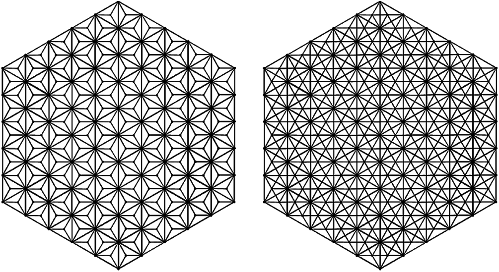
Figure 6: HDN1(n) and HDN2(n) networks
The HDN1(n) is a planar graph and was shown to have
Here |R|, represents the upper bound of the proposed resolving set for the hex derived network HDN1(n), and k is any positive integer.
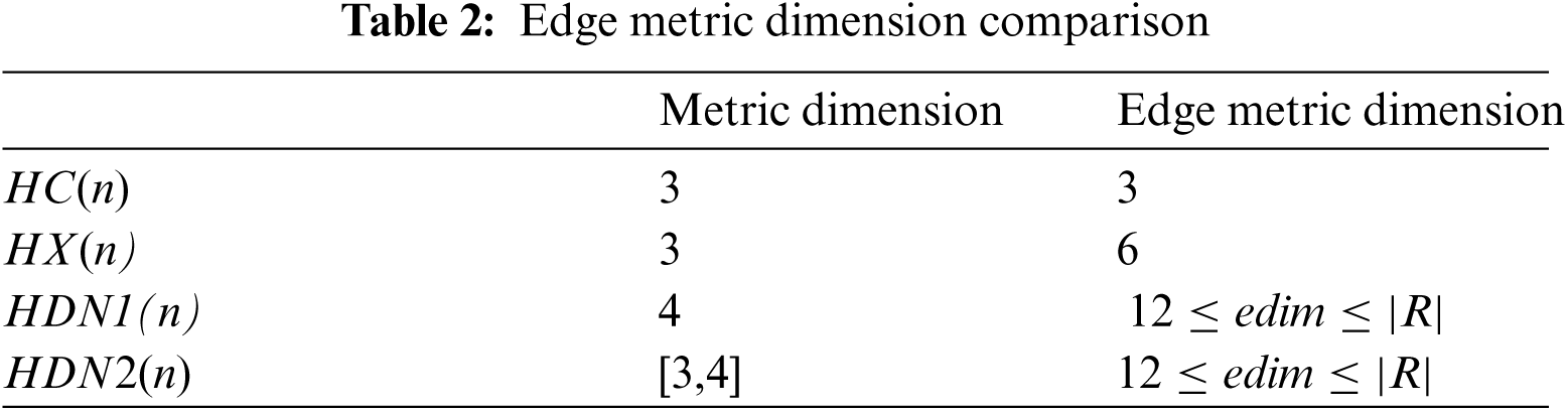
The comparison of the research is summarized in Tab. 2. It is observed that the Metric dimension of HC(n) proposed in [41] and the edge metric dimension of these networks as proved in this research are the same. However, this research shows that the edge metric dimension of the HX(n) is greater than the metric dimension of HX(n) which was found out to be 3 in [41]. While [42] was able to give a bound for both the hex derived networks and [43] found the exact value for HDN1(n) networks and this research is able to find the bounds for the HDN1(n) networks.
In this paper the edge metric dimension of honeycomb and hexagonal networks were studied which could effectively be utilized by wireless sensor networks in a IoT scenario, such as robot/drone navigation. After representing the network via a graph in terms of robots and landmarks, a robot could measure its distance in the graph to any landmark. The objective was to enable robot in finding out the fewest number of landmarks in order to determine its current node thereby using only the distances to the landmarks. It was proved that the minimum landmarks required for a honeycomb network HC(n) and a hexagonal network HX(n) are 3 and 6, respectively. The bounds were proposed for the landmarks required for the hex-derived network HDN1(n), i.e., by finding out the resolving set for the network of HDN1(n). However, the exact values of the number of landmarks required for hex derived networks are still unfound and the methodology proposed for the number of landmarks required for hex networks cannot be naturally extended to hex derived networks. Since the hex derived networks are more efficient in an IoT scenario, exact values for the number of landmarks for these hex-derived networks point towards a future direction of research.
Acknowledgement: The authors thank their families and colleagues for their continued support.
Funding Statement: No funding was received to support any stage of this research study. Zahid Raza is funded by the University of Sharjah under the Projects #2102144098 and #1802144068 and MASEP Research Group.
Conflicts of Interest: The authors declare that they have no conflicts of interest to report regarding the present study.
1. B. Selcuk, A. N. A. Tankul and A. Karci, “Topology properties of hierarchical honeycomb meshes,” in CEUR Workshop Proceedings, vol. 2864, pp. 485–495, 2021. [Google Scholar]
2. F. Khan, S. Abbas and S. Khan, “An efficient and reliable core-assisted multicast routing protocol in mobile ad-hoc network,” International Journal of Advanced Computer Science and Applications, vol. 7, no. 5, pp. 231–242, 2016. [Google Scholar]
3. F. Khan, A. W. Khan, S. Khan, I. Qasim and A. Habib, “A secure core-assisted multicast routing protocol in mobile ad-hoc network,” Journal of Internet Technology, vol. 21, no. 2, pp. 375–83, 2020. [Google Scholar]
4. A. Rashid, F. Khan, T. Gul, S. Khan and F. K. Khalil, “Improving energy conservation in wireless sensor networks using energy harvesting system,” International Journal of Advanced Computer Science and Applications, vol. 9, no. 1, pp. 354–361, 2018. [Google Scholar]
5. F. Javed, S. Khan, A. Khan, A. Javed, R. Tariq et al., “On precise path planning algorithm in wireless sensor network,” International Journal of Distributed Sensor Networks, vol. 14, no. 7, pp. 1–12, 2018. [Google Scholar]
6. S. M. Hussain, A. Wahid, M. A. Shah, A. Akhunzada et al., “Seven pillars to achieve energy efficiency in high-performance computing data centers,” Recent Trends and Advances in Wireless and IoT-Enabled Networks, vol. 92, pp. 93–105, 2019. [Google Scholar]
7. B. S. Tripathi, M. K. Shukla and M. K. Srivastava, “Performance enhancement in wireless sensor network using hexagonal topology,” in IEEE Int. Conf. Communication, Control and Intelligent Systems, Mathura, India, pp. 113–119, 2016. [Google Scholar]
8. V. Soni and D. K. Mallick, “An optimal geographic routing protocol based on honeycomb architecture in wireless sensor networks,” in IEEE Int. Conf. on Electrical, Electronics, and Optimization Techniques, Chennai, India, pp. 4440–4444, 2016. [Google Scholar]
9. A. Rais, K. Bouragba and M. Ouzzif, “Routing and clustering of sensor nodes in the honeycomb architecture,” Journal of Computer Networks and Communications, vol. 2019, pp. 1–13, 2019. [Google Scholar]
10. S. K. Biswash and C. Kumar, “An efficient metric-based (EM-B) location management scheme for wireless cellular networks,” Journal of Network and Computer Applications, vol. 34, no. 6, pp. 2011–2026, 2011. [Google Scholar]
11. R. d. Rosa, M. A. Wehrmeister, T. Brito, J. L. Lima and A. I. P. N. Pereira, “Honeycomb map: A bioinspired topological map for indoor search and rescue unmanned aerial vehicles,” Sensors, vol. 20, no. 3, pp. 907–930, 2020. [Google Scholar]
12. E. Kadioglu, C. Urtis and N. Papanikolopoulos, “UAV coverage using hexagonal tessellation,” in 27th Mediterranean Conf. on Control and Automation, Akko, Israel, pp. 37–42, 2019. [Google Scholar]
13. S. M. Amini, A. Karimi and M. Esnaashari, “Energy-efficient data dissemination algorithm based on virtual hexagonal cell-based infrastructure and multi-mobile sink for wireless sensor networks,” Journal of Supercomputing, vol. 76, no. 1, pp. 150–173, 2020. [Google Scholar]
14. O. C. Mathew and A. M. J. Z. Rahman, “A novel energy optimization mechanism for medical data transmission using honeycomb routing,” Journal of Medical Imaging and Health Informatics, vol. 6, no. 3, pp. 857–862, 2016. [Google Scholar]
15. C. Zhu, G. Han and H. Zhang, “A honeycomb structure based data gathering scheme with a mobile sink for wireless sensor networks,” Peer-to-Peer Networking and Applications, vol. 10, no. 3, pp. 484–499, 2017. [Google Scholar]
16. Y. Zhuang, T. A. Gulliver and Y. Coady, “On planar tessellations and interference estimation in wireless ad-hoc networks,” IEEE Wireless Communications Letters, vol. 2, no. 3, pp. 331–334, 2013. [Google Scholar]
17. A. M. Khedr, W. Osamy, A. Salim and S. Abbas, “A novel association rule-based data mining approach for internet of things based wireless sensor networks,” IEEE Access, vol. 8, pp. 151574–151588, 2020. [Google Scholar]
18. H. Harb, C. A. Jaoude and A. Makhoul, “An energy-efficient data prediction and processing approach for the internet of things and sensing based applications,” Peer-to-Peer Networking and Applications, vol. 13, no. 3, pp. 780–795, 2020. [Google Scholar]
19. F. Kiani and A. Seyyedabbasi, “Wireless sensor network and internet of things in precision agriculture,” International Journal of Advanced Computer Science and Applications, vol. 9, no. 6, pp. 99–103, 2018. [Google Scholar]
20. E. Akanksha, “HNM: Hexagonal network model for comprehensive smart city management in internet-of-things,” Advances in Intelligent Systems and Computing, vol. 1224, pp. 542–553, 2020. [Google Scholar]
21. K. Shafique, B. A. Khawaja, F. Sabir, S. Qazi and M. Mustaqim, “Internet of things (IoT) for next-generation smart systems: A review of current challenges, future trends and prospects for emerging 5G-IoT scenarios,” IEEE Access, vol. 8, pp. 23022–23040, 2020. [Google Scholar]
22. S. Ahmad, S. Malik, I. Ullah, D. H. Park, D. Kim et al., “Towards the design of a formal verification and evaluation tool of real-time tasks scheduling of IoT applications,” Sustainability, vol. 11, no. 1, pp. 204–231, 2019. [Google Scholar]
23. F. Mehmood, S. Ahmad and D. Kim, “Design and implementation of an interworking IoT platform and marketplace in cloud of things,” Sustainability, vol. 11, no. 21, pp. 5952–5973, 2019. [Google Scholar]
24. S. Ahmad, S. Malik, I. Ullah, M. Fayaz, D.-H. Park et al., “An adaptive approach based on resource-awareness towards power-efficient real-time periodic task modeling on embedded IoT devices,” Processes, vol. 6, no. 7, pp. 90–118, 2018. [Google Scholar]
25. S. Khuller, B. Raghavachari and A. Rosenfeld, “Landmarks in graphs,” Discrete Applied Mathematics, vol. 70, no. 3, pp. 217–229, 1996. [Google Scholar]
26. A. Otto, N. Agatz, J. Campbell, B. Golden and E. Pesch, “Optimization approaches for civil applications of unmanned aerial vehicles (UAVs) or aerial drones: A survey,” Networks, vol. 72, no. 4, pp. 411–458, 2018. [Google Scholar]
27. S. I. Ktena, S. Parisot, E. Ferrante, M. Rajchl, M. Lee et al., “Metric learning with spectral graph convolutions on brain connectivity networks,” NeuroImage, vol. 169, pp. 431–442, 2018. [Google Scholar]
28. N. Zubrilina, “On the edge dimension of a graph,” Discrete Mathematics, vol. 341, no. 7, pp. 2083–2088, 2018. [Google Scholar]
29. A. Kelenc, D. Kuziak, A. Taranenko and I. G. Yero, “Mixed metric dimension of graphs,” Applied Mathematics and Computation, vol. 314, pp. 429–438, 2017. [Google Scholar]
30. Z. Raza and N. Siddiqui, “The edge metric dimension of cayley graphs and its barycentric subdivisions,” Nonlinear Functional Analysis and Applications, vol. 24, no. 4, pp. 801–811, 2019. [Google Scholar]
31. M. S. Bataineh, N. Siddiqui and Z. Raza, “Edge metric dimension of k multiwheel graph,” Rocky Mountain Journal of Mathematics, vol. 50, no. 4, pp. 1175–1180, 2020. [Google Scholar]
32. M. S. Chen, K. G. Shin and D. D. Kandlur, “Addressing, routing, and broadcasting in hexagonal mesh multiprocessors,” IEEE Transactions on Computers, vol. 39, no. 1, pp. 10–18, 1990. [Google Scholar]
33. I. Stojmenovic, “Honeycomb networks: Topological properties and communication algorithms,” IEEE Transactions on Parallel and Distributed Systems, vol. 8, no. 10, pp. 1036–1042, 1997. [Google Scholar]
34. Z. Raza, M. S. Bataineh and M. E. Sukaiti, “On the zagreb connection indices of hex and honeycomb networks,” Journal of Intelligent and Fuzzy Systems, vol. 40, no. 3, pp. 4107–4114, 2021. [Google Scholar]
35. I. Peterin and I. G. Yero, “Edge metric dimension of some graph operations,” Bulletin of the Malaysian Mathematical Sciences Society, vol. 43, no. 3, pp. 2465–2477, 2020. [Google Scholar]
36. F. Okamoto, B. Phinezy and P. Zhang, “The local metric dimension of a graph,” Mathematica Bohemica, vol. 135, no. 3, pp. 239–255, 2010. [Google Scholar]
37. I. G. Yero, “On the strong partition dimension of graphs,” arXiv preprint arXiv:1312.1987, pp. 1–16, 2013. [Google Scholar]
38. A. Kelenc, N. Tratnik and I. G. Yero, “Uniquely identifying the edges of a graph: The edge metric dimension,” Discrete Applied Mathematics, vol. 251, pp. 204–220, 2018. [Google Scholar]
39. M. R. Chithra and M. K. Menon, “Secure domination of honeycomb networks,” Journal of Combinatorial Optimization, vol. 40, no. 1, pp. 98–109, 2020. [Google Scholar]
40. F. G. Nocetti, I. Stojmenovic and J. Zhang, “Addressing and routing in hexagonal networks with applications for tracking mobile users and connection rerouting in cellular networks,” IEEE Transactions on Parallel and Distributed Systems, vol. 13, no. 9, pp. 963–971, 2002. [Google Scholar]
41. P. Manuel, R. Bharati, I. Rajasingh and C. Monica, “On minimum metric dimension of honeycomb networks,” Journal of Discrete Algorithms, vol. 6, no. 1, pp. 20–27, 2008. [Google Scholar]
42. J. Xu and D. Fan, “On the metric dimension of HDN,” Journal of Discret Algorithms, vol. 26, pp. 1–6, 2014. [Google Scholar]
43. Z. Shao, P. Wu, E. Zhu and L. Chen, “On metric dimension in some hex derived networks,” Sensors, vol. 19, no. 1, pp. 94–105, 2019. [Google Scholar]
 | This work is licensed under a Creative Commons Attribution 4.0 International License, which permits unrestricted use, distribution, and reproduction in any medium, provided the original work is properly cited. |