DOI:10.32604/cmc.2022.022952
| Computers, Materials & Continua DOI:10.32604/cmc.2022.022952 | |
| Article |
Deep Reinforcement Learning for Addressing Disruptions in Traffic Light Control
1School of Engineering and Computer Science, University of Hertfordshire, Hatfield, AL109AB, UK
2Department of Computing and Information Systems, Sunway University, Subang Jaya, 47500, Malaysia
3Faculty of Computer Science and Information Technology, University of Malaya, Kuala Lumpur, 50603, Malaysia
4National Advanced IPv6 Centre, Universiti Sains Malaysia, USM, Penang, 11800, Malaysia
*Corresponding Author: Yung-Wey Chong. Email: chong@usm.my
Received: 24 August 2021; Accepted: 27 September 2021
Abstract: This paper investigates the use of multi-agent deep Q-network (MADQN) to address the curse of dimensionality issue occurred in the traditional multi-agent reinforcement learning (MARL) approach. The proposed MADQN is applied to traffic light controllers at multiple intersections with busy traffic and traffic disruptions, particularly rainfall. MADQN is based on deep Q-network (DQN), which is an integration of the traditional reinforcement learning (RL) and the newly emerging deep learning (DL) approaches. MADQN enables traffic light controllers to learn, exchange knowledge with neighboring agents, and select optimal joint actions in a collaborative manner. A case study based on a real traffic network is conducted as part of a sustainable urban city project in the Sunway City of Kuala Lumpur in Malaysia. Investigation is also performed using a grid traffic network (GTN) to understand that the proposed scheme is effective in a traditional traffic network. Our proposed scheme is evaluated using two simulation tools, namely Matlab and Simulation of Urban Mobility (SUMO). Our proposed scheme has shown that the cumulative delay of vehicles can be reduced by up to 30% in the simulations.
Keywords: Artificial intelligence; traffic light control; traffic disruptions; multi-agent deep Q-network; deep reinforcement learning
Traffic congestion has become a problem in most urban areas of the world, causing enormous economic waste, extra travel delay, and excessive vehicle emission [1]. The traffic light controllers, which are installed to monitor and control the traffic flows at intersections in order to alleviate traffic congestion strategically. Each traffic light controller has: a) light colors in which green color represents “go”, amber represents “slow down”, and red represents “stop”; b) traffic phase, in which a set of green lights are assigned to a set of lanes for safe and non-conflicting movements at the intersections; and c) traffic phase split is the time period of a traffic phase. The traffic phase split includes a short moment of red lights for all lanes to provide a safe transition in between traffic phases. The time passed since the respective lane light has changed to red is represented by red timing.
Next, we present five main fundamentals related to our investigation in the use of MADQN to traffic light controllers for reducing the cumulative delay of vehicles. Firstly, various types of traffic light controllers are presented to control and alleviate traffic congestion. Secondly, various artificial intelligence approaches are presented to accomplish fully-dynamic traffic light controllers. Thirdly, the traditional DQN approach is presented as an enhanced artificial intelligence approach applied to traffic light controllers. Fourthly, the significance of using the cumulative delay of vehicles as the performance measure is presented. Fifthly, traffic disruptions to traffic network are introduced using the Burr distribution. The contributions of this paper are also presented.
1.1 Types of Traffic Light Controllers
Traditionally, traffic light controllers monitor traffic movements and determine traffic phase splits to control and reduce congestion in traffic by using three main techniques. Firstly, a deterministic traffic light controller is a pretimed control system that uses historical data of traffic collected at different times and determines traffic phase splits using the Webster formula [2]. Secondly, a semi-dynamic traffic light controller is a system based on actuated control, and it uses instantaneous or short-term traffic condition, such as the absence and presence of vehicles, and assigns green lights to lanes with vehicles [3]. The short-term traffic condition can be detected using an inductive loop detector. Thirdly, a fully-dynamic traffic light controller is also a system based on actuated control; however, it uses longer-term traffic condition, including the average queue length and waiting time of vehicles of a lane. The longer-term traffic condition (e.g., the average queue length and the waiting time of vehicles at a lane) can be measured by the number of vehicles using at least two inductive loop detectors at a lane, one is installed near the intersection and another one is installed further away from the intersection [4]. By measuring the number of vehicles, the average queue length and waiting time of vehicles at a lane can be calculated. Video-based traffic detector (or camera sensor) can also be installed at an intersection, and image processing can be used to calculate the number of vehicles at a lane of an intersection [5]. Subsequently, it adjusts the traffic phase split based on the traffic condition [6]. The fully-dynamic traffic light controllers are more realistic in monitoring traffic movements because it uses longer-term traffic conditions, and the approach has shown to alleviate traffic congestion more effectively compared to deterministic and semi-dynamic traffic light controllers [7–9].
1.2 Common Approaches of Fully-Dynamic Traffic Light Controllers
The fully-dynamic traffic light controller has commonly been accomplished using artificial intelligence approaches, particularly reinforcement learning (RL) [10,11] and multi-agent reinforcement learning (MARL) [12]. RL can be embedded in a single agent (or a decision maker), which is the traffic light controller, to learn, make optimal action (i.e., traffic phase split), and improve its operating environment (i.e., the local traffic condition). In contrast, MARL can be embedded in multiple traffic light controllers (or agents) to exchange knowledge (i.e., Q-values), learn, make optimal joint action, and improves their operating environment (i.e., the global traffic condition) in a collaboration. However, the curse of dimensionality has occurred in single-agent RL and MARL, in which the state space is too large to be handled efficiently due to the complexity of the traffic congestion issue [13], and so this paper uses multi-agent deep Q-network (MADQN) that is based on the traditional single-agent DQN approach [14]. This paper extends our previous work [15] that mainly focuses on measuring the performance measures, such as throughput, waiting time, and queue length, which are unable to relate to drivers’ experience. This paper investigates the use of MADQN to traffic light controllers at intersections with high volume of traffic and traffic disruptions (i.e., rainfall) by measuring the cumulative delay of vehicles as the performance measure, which relate to drivers’ experience.
1.3 DQN as an Enhanced RL-Based Approach for Traffic Light Controllers
DQN is a combination of the new evolving deep learning technique [16] and the traditional RL technique, conveniently called deep reinforcement learning (DRL) [17]. DQN solves the curse of dimensionality and provides two main advantages [18]: a) reduces the learning time and computational cost incurred to explore different pairs of state-action and identify the actions that are optimal; and b) uses hidden layers to provide abstract and continuous representations of the complex and high-dimensional inputs (i.e., the state space) for reducing the capacity of storage needed to store the unlimited number of pairs of state-action (or the Q-values).
1.4 Cumulative Delay of Vehicles as the Performance Measure Used by Traffic Light Controllers
The cumulative delay of the vehicles is the average time (i.e., average travelling and waiting times caused by congestion) taken by vehicles to travel from a source location to a destination location, which may require crossing multiple intersections. Compared to other measures, including the average queue length and waiting time of the vehicles of a lane, and throughput (i.e., the number of vehicles crossing an intersection), the cumulative delay can be directly perceived by drivers, and so it relates to the drivers’ experiences. In other words, drivers perceive the difference between the actual and expected travel times when crossing multiple intersections. The investigations with respect to the cumulative delay of vehicles as the performance measure has gained momentum over the years with the use of DRL to traffic light control. Specifically, the cumulative delay is the most frequently used performance measure in the literature from January 2016 to November 2020 as compared to other performance measures in the investigation of the use of DRL to traffic light control as shown in Fig. 1. The scientific literature databases, including Web of Science [19], IEEE Xplore Digital Library [20], and ScienceDirect [21], have been used to conduct this study. The cumulative delay of vehicles has gained momentum over the years due to its better reflection of the real circumstances, particularly the drivers’ experiences. While the cumulative delay has been used in the literature [22,23], it has not been applied to traffic congestion at multiple intersections scenario under the presence of increased traffic volume and traffic disruptions, and so this paper adopts this measure to calculate the average time required by vehicles to cross multiple intersections.
1.5 Burr Distribution for Introducing Traffic Disruptions to Traffic Networks
Traffic congestion can be categorized into: a) recurrent congestion (RC) caused by the high volume of traffic; and b) non-recurrent congestion (NRC) caused by erratic traffic disruptions, including accidents, and rainfall [24,25]. In the literature [26], the arrival process of vehicles has been widely modeled by the Poisson process, whereby the inter-arrival time of vehicles follows an exponential distribution. The Poisson process incorporates RC naturally; however, it does not incorporate NRC, and so the Burr distribution, which is the generalization of the Poisson process, has been adopted by this work to model the vehicle’s time of inter-arrival under scenarios with a high volume of traffic (i.e., RC) and traffic disruptions (i.e., NRC).
1.6 Contributions of the Paper
Our contribution is to investigate the use of MADQN to traffic light controllers at intersections with a high volume of traffic and traffic disruptions (i.e., rainfall). This work is based on simulation using the Burr distribution, which has been shown to model traffic disruptions in traffic networks accurately in [27]. The performance measure is the cumulative delay of vehicles, which includes the average waiting and travelling times caused by congestion. This performance measure is used because the difference between the actual and expected travel times when crossing multiple intersections can be directly perceived by drivers, and so it relates to the drivers’ experiences. In this paper, we aim to show a performance comparison between MADQN and MARL applied to traffic light controllers at intersections with a high volume of traffic and traffic disruptions in terms of the cumulative delay of vehicles, which has not been investigated in the literature despite its significance.
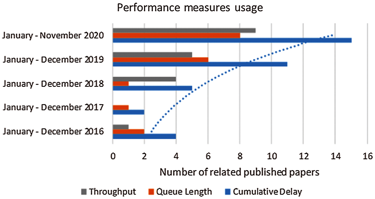
Figure 1: The usage of three popular performance measures in the investigation of the use of DRL to traffic light control in recent years
The paper is structured into six sections.
• Section 1 presents the introduction of traffic light controllers and the background of common approaches for traffic light controllers. It also presents the contributions of the paper.
• Section 2 presents the background of the Krauss vehicle-following model, DRL and MARL. The traditional algorithms of DRL and MARL are also presented in this section.
• Section 3 presents the literature review of DQN-based traffic light controllers. There are five main DQN approaches discussed in this section.
• Section 4 presents the proposed MADQN model for traffic light controllers. It presents the representations of the proposed MADQN model, including the state space, action space, and delayed reward, applied to traffic light controllers. It also presents the MADQN architecture and algorithm.
• Section 5 presents an application for sustainable city (i.e., Sunway city), and our simulation results and discussion.
• Section 6 concludes this paper with a discussion of potential future directions.
This section presents the background of the Krauss vehicle-following model, DRL and MARL. The Krauss vehicle-following model is a mathematical model of safe vehicular movement, whereby a gap between two consecutive vehicles is maintained. The background of DRL includes the traditional single-agent deep Q-network (DQN) algorithm. The background of MARL includes its traditional algorithm.
2.1 Krauss Vehicle-Following Model
In 1997, Krauss developed a vehicle-following model based on the safe speed of vehicles. The safe speed is calculated as follows [28]:
where
In our study, the Krauss vehicle-following model is used to ensure the safe movement of vehicles at intersections of the Sunway city and grid traffic networks (see Section 5).
2.2 Deep Reinforcement Learning
DRL incorporates DNNs into RL that enables agents to learn relationships between actions and states. DeepMind has first proposed the DQN [17], which is the DRL method, and it has been widely adopted in traffic light control [29]. DQN consists of a DNN, which is comprised of three main kinds of layers, namely the input layer, hidden layer(s), and output layer. In DQN, the neurons are interconnected with each other and they can learn complex and unstructured data [30]. During training, the data flows from the input layer to the hidden layer(s), and finally to the output layer. DQN provides two main features, which are: a) experience replay, in which experiences are stored in a replay memory, and then the experiences are randomly selected for training; and b) target network, which is the main network duplicate. The main network selects actions based on observations from the operating environment and updates its weights. The target network approximates the weights of the main network to generate its Q-value. During training, the Q-value of the target network is used to calculate the loss incurred by a selected action, and it has shown to stabilize training. After every certain number of iterations, the target network is updated. The main difference between the main and target networks is that the main network is used during observation, action selection and training processes, while the target network is used during training process only.
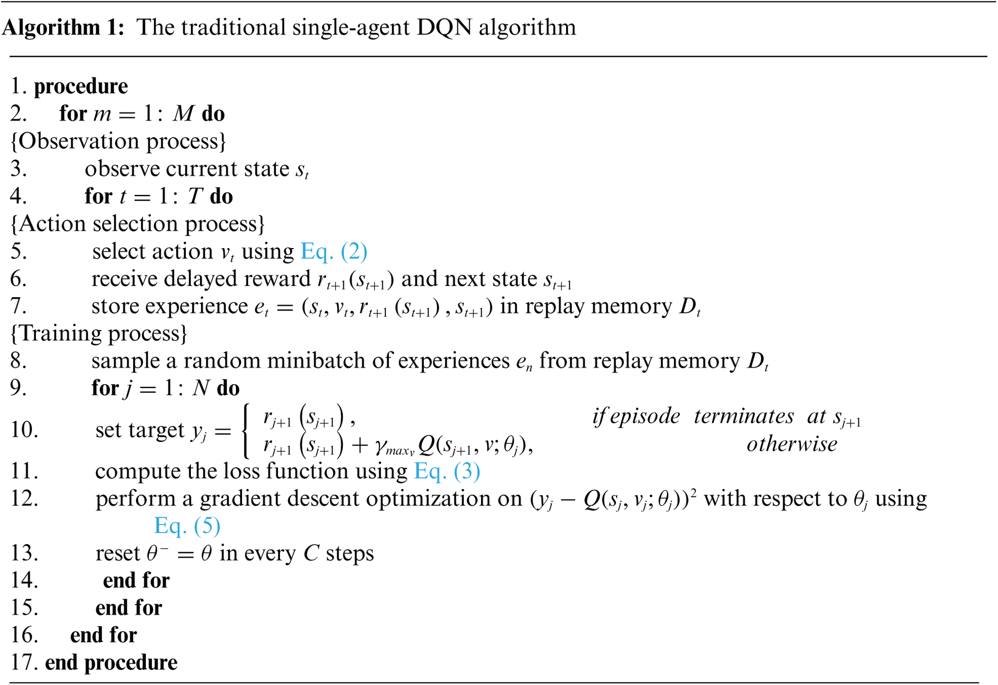
Algorithm 1 shows the DQN algorithm. In
where
where
where
The target Q-values
2.3 Multi-Agent Reinforcement Learning
MARL is an extended approach of the traditional RL approach that enables multiple agents to exchange information with each other in order to achieve the optimal network-wide performance [32]. The optimization of the network-wide objective function is the main purpose, such as the global Q-value that sums up the local Q-values of all agents in a single network, as time goes by
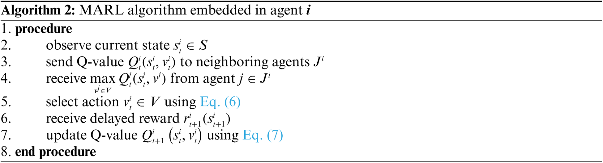
Agent
where
where
This section presents a literature review of DQN-based traffic light controllers, which have shown to achieve various performance measures. Five main DQN approaches have been proposed to reduce the cumulative delay of vehicles. In general, the DQN approaches are embedded in traffic light controllers. The DQN model has an input layer that receives state, and an output layer that provides Q-values for possible actions (e.g., traffic phases [33] and traffic phase splits [34]).
The application of the traditional DNN-based DQN approach to traffic light control is proposed in [33,35]. In the Wan’s DNN-based DQN model [33]: a) state represents the current traffic phase, the queue length, and the green and red timings; b) action represents a traffic phase; and c) reward represents the waiting time of vehicles. In the Tan’s DNN-based DQN model [35]: a) state represents the queue length of vehicles; b) action represents a traffic phase; and c) reward represents the queue length and waiting time, as well as throughput. The proposed schemes have shown to reduce the cumulative delay [33,35] and queue length [35] of vehicles, and improve throughput [33].
The convolutional neural network (CNN)-based DQN approach enables agents to analyze visual imagery of traffic in an efficient manner. The agents process the input states, which are represented in the form of a two-dimensional matrix (i.e., multiple rows and columns of values, such as an image) or one-dimensional vectors (e.g., a single row or column of values, such as the queue length of a lane) [29]. The application of the CNN-based DQN approach to traffic light control is proposed in [22], [23,34,36]. In the Genders’ and Gao’s CNN-based DQN model [22,34]: a) state represents the current traffic phase, as well as the position and speed of vehicles; b) action represents a traffic phase [22] and a traffic phase split [34]; and c) reward represents the waiting time of vehicles. In the Wei’s CNN-based DQN model [36]: a) state represents the current traffic phase, as well as the position and queue length of vehicles; b) action represents a traffic phase; and c) reward represents the waiting time and queue length. In the Mousavi’s CNN-based DQN model [23]: a) state represents the current traffic phase and queue length; b) action represents a traffic phase; and c) reward represents the waiting time of vehicles. The proposed schemes have shown to reduce the cumulative delay [22,23,34,36], waiting time [34], and queue length [22,23,36] of vehicles, as well as improve throughput [22,36].
The stacked auto encoder (SAE) neural network-based DQN approach enables agents to perform encoding and decoding functions, and store inputs efficiently. The application of the SAE neural network-based DQN approach to traffic light control is proposed in [37]. In the Li’s SAE neural network-based DQN model [37]: a) state represents the queue length; b) action represents a traffic phase split; and c) reward represents the queue length and waiting time. The simulation results have shown that the proposed scheme can reduce the cumulative delay and queue length of vehicles.
The long short-term memory (LSTM) neural network-based DQN approach enables agents to memorize previous inputs of a traffic light control using a memory cell that maintains a time window of states. The advantage of the actor critic (A2C)-based method is that it is a combination of value-based and policy-gradient (PG)-based DQN method. Each agent has an actor that controls how it behaves (i.e., PG-based), and a critic that measures the suitability of the selected action (i.e., value-based). The application of the LSTM neural network-based DQN with A2C approach to traffic light control has been proposed in [38]. In [38]: a) state represents the queue length; b) action represents a traffic phase; and c) reward represents the queue length and waiting time. The simulation results have shown that the proposed scheme can reduce the cumulative delay and queue length of vehicles, as well as improve throughput.
The MADQN approach allows multiple DQN agents to share knowledge (i.e., Q-values), learn, and make optimal joint actions (i.e., traffic phase split) in a collaboration. In the Rasheed’s MADQN model [15]: a) state represents queue length, the current traffic phase, red timing, and the rainfall intensity; b) action represents a traffic phase split; and c) reward represents the waiting time of the vehicles. The simulation results have shown that the proposed scheme can reduce the waiting time and queue length at a lane, and improve throughput. In this paper, we extend the work in [15] by evaluating the cumulative delay of vehicles incurred by MARL and MADQN at multiple intersections, while having traffic disruptions (i.e., rainfall).
4 Our Proposed MADQN Approach for Traffic Light Controllers
In a traffic network, an intersections set
MADQN has three main advantages as compared to MARL as follows:
• MADQN uses DNNs, which provide the state space with its continuous representation. Consequently, it represents an unlimited number of pairs of state-action.
• MADQN addresses the curse of dimensionality by providing efficient storage for complex inputs.
• MADQN uses a target network with experience replay, and so it improves the stability of training.
The remainder of this subsection presents the representations of the state, action, and delayed reward of the MADQN model at an intersection
The state
•
•
•
•
•
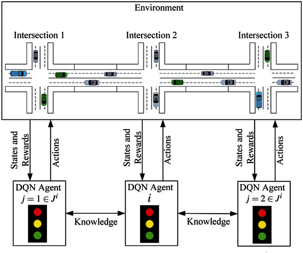
Figure 2: An abstract model of agent
The action
An agent receives delayed rewards that vary with the average waiting time of the vehicles at the intersections. Traffic congestion can cause an increment in the average waiting time of the vehicles at the intersections. The delayed reward
Fig. 3 shows the DQN architecture. There are three main components in an agent, namely the main network, the target network, and the replay memory. The main network consists of a DNN with its weight
The DNN has three kinds of layers (see Section 2). In our DQN architecture, there are
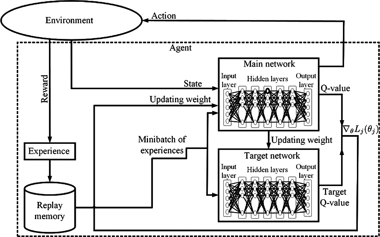
Figure 3: DQN architecture
In this section, the extension of the traditional DQN approach to MADQN for multiple intersections is presented, and it has not been explored in the literature. The proposed MADQN algorithm is evaluated in simulation under different traffic networks (see Section 5) in the presence of traffic disruptions.
MADQN allows knowledge to be learned and exchanged among multiple DQN agents for coordination. The traditional MARL approach enables an agent to choose an optimal action based on its neighboring agents’ actions. In the moving target scenario, actions are selected independently by agents simultaneously, and so the action selected by an agent
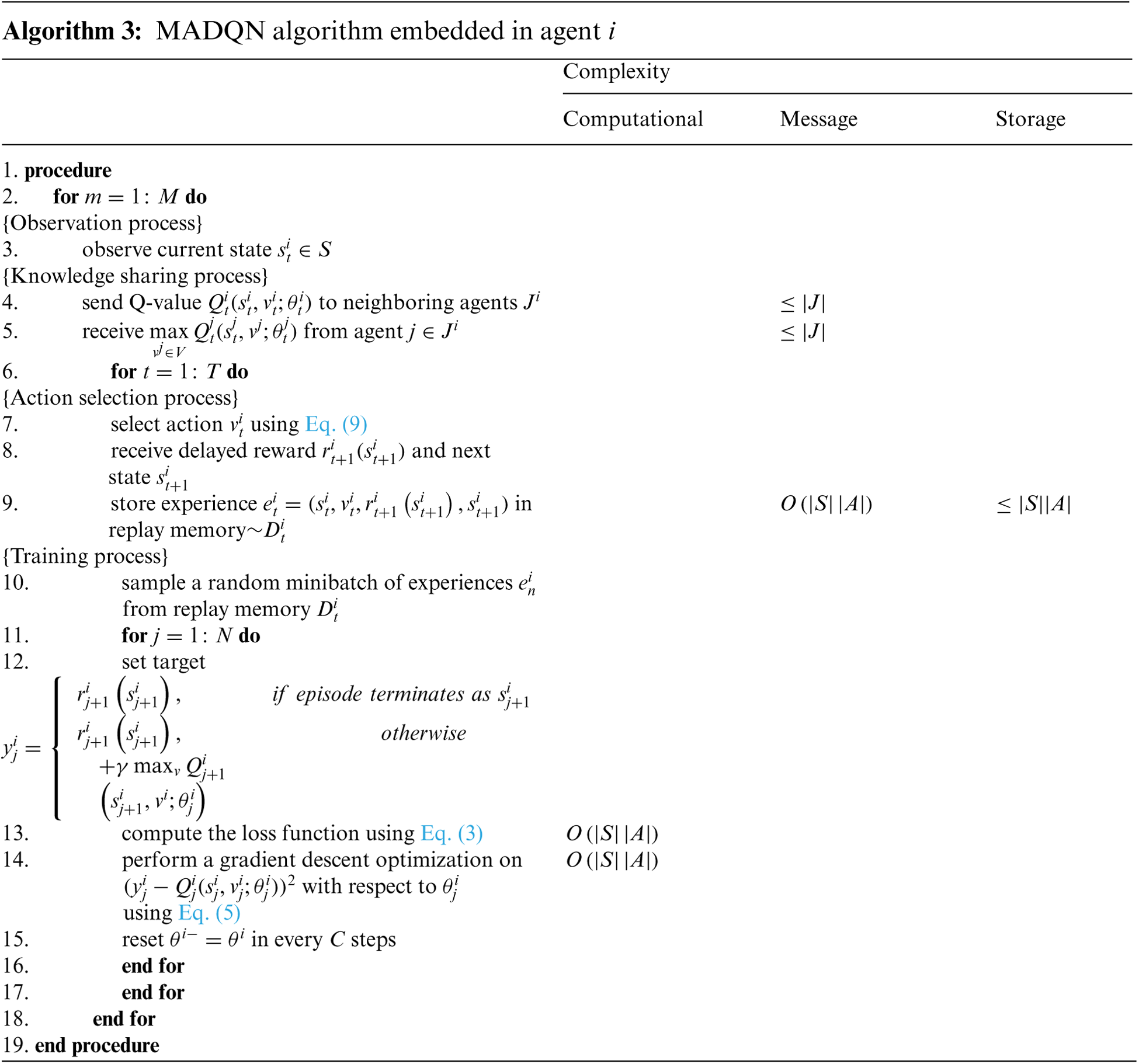
Algorithm 3 shows the algorithm for MADQN, which is an extension of Algorithm 2. In episode
where
where
The proposed MADQN algorithm allows an agent to receive Q-values from neighboring agents and use them to select the optimal action.
This section presents an analysis of the computational, message, and storage complexities of the proposed MADQN algorithm (i.e., Algorithm 3) applied to traffic light controllers. In this paper, the complexity analysis has two levels: a) step-wise that considers a single execution or iteration of the MADQN algorithm; and b) agent-wise that considers all the state-action pairs of an agent. Note that, only exploitation actions are considered while analyzing the algorithm.
Computational complexity estimates the maximum number of iterations, episodes, and so on, executed to calculate Q-values under all possible states. The step-wise computational complexity is considered under a particular state. An agent
Message complexity is the number of messages exchanged between the agents in order to calculate the Q-values. An agent
Storage complexity is the amount of memory needed to store knowledge (i.e., Q-values) and the experiences of agents. An agent
5 Application for Sustainable City and Simulation Results
An investigation of the proposed scheme has been conducted in a case study based on a real traffic network, which is part of a sustainable urban city project in the Sunway City of Kuala Lumpur in Malaysia. Investigation is also performed using a grid traffic network (GTN) to understand the performance of the proposed scheme in a complex traffic network. Hence, our investigation covers both real-world and complex traffic networks, which are based on simulation. In this paper, the traffic networks with a left-hand traffic is considered, in which the traffic movement for the left turn is either protected or does not conflict with other traffic movements. This section also presents simulation results and discussion for our simulation in both RC and NRC environments.
5.1 Sunway City in Kuala Lumpur
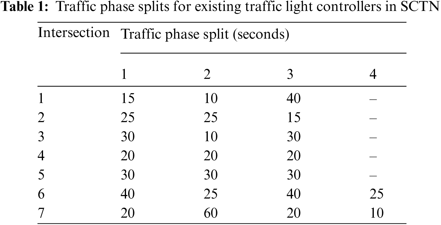
Sunway city is one of the sustainable and smart cities in Malaysia [40]. It has busy commercial areas, residential areas with high density (i.e., LaCosta and Sunway Monash Residence), higher educational institutions (i.e., Monash University Malaysia campus and Sunway University), health centre (i.e., Sunway Medical Centre), amusement park (i.e., Sunway Lagoon), hotel (i.e., Sunway Resort Hotel & Spa), and so on, as shown in Fig. 4. In Fig. 4, the Sunway city traffic network (SCTN) has seven intersections, whereby every intersection has a traffic light controller. Fig. 5 shows the traffic phases, and Tab. 1 shows the traffic phase splits of existing (i.e., deterministic) traffic light controllers at all intersections in SCTN. The traffic phase splits were observed during the evening busy hours (i.e., 5–7 pm) of a working day, and they were measured using a stopwatch.
Malaysia ranks third and fifth worldwide in the number of lightning strikes (i.e., around 240 thunderstorm days/year [41]) and rainfall (i.e., around 1000 mm/year [42]), respectively. So, traffic congestion caused by traffic disruptions (i.e., rainfall) during the peak hours is a serious problem.
In this paper, we apply our proposed algorithm to the traffic network of Sunway city. Investigation is conducted in the traffic simulator SUMO [43].
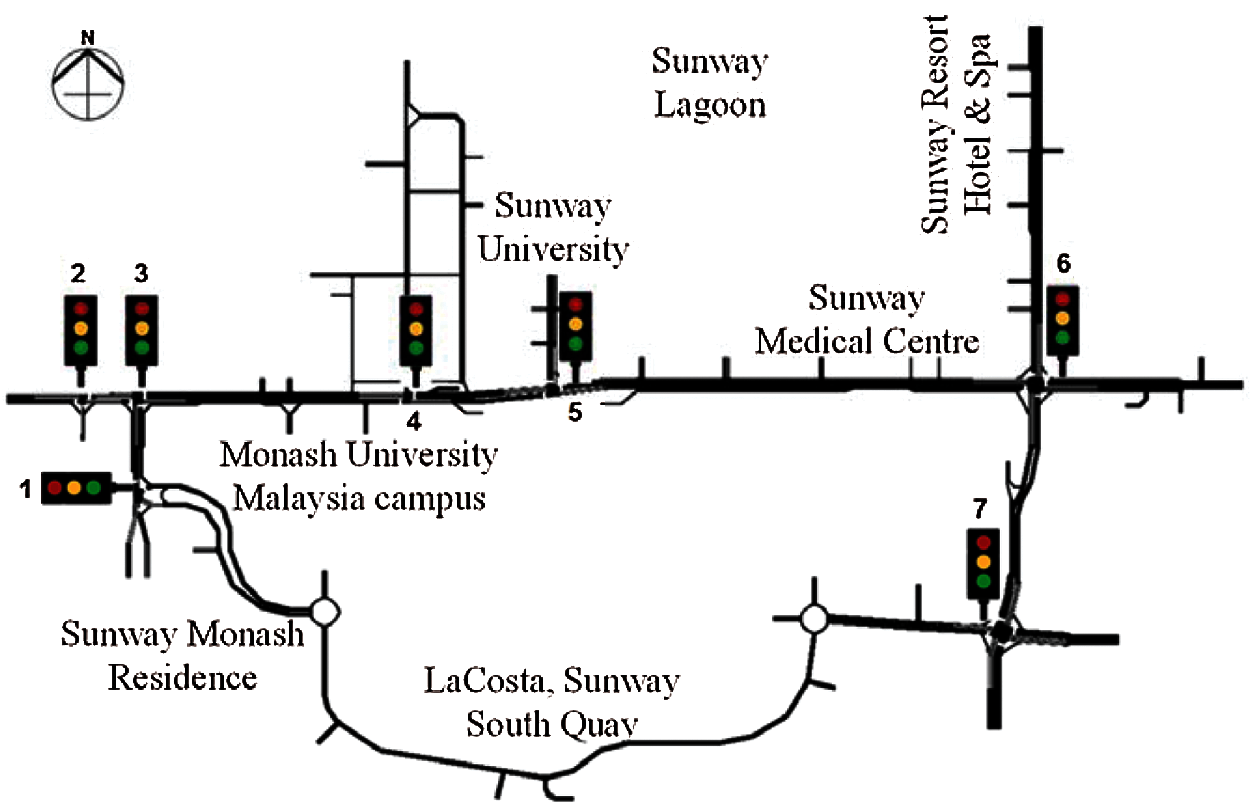
Figure 4: A SCTN and the locations of its traffic light controllers
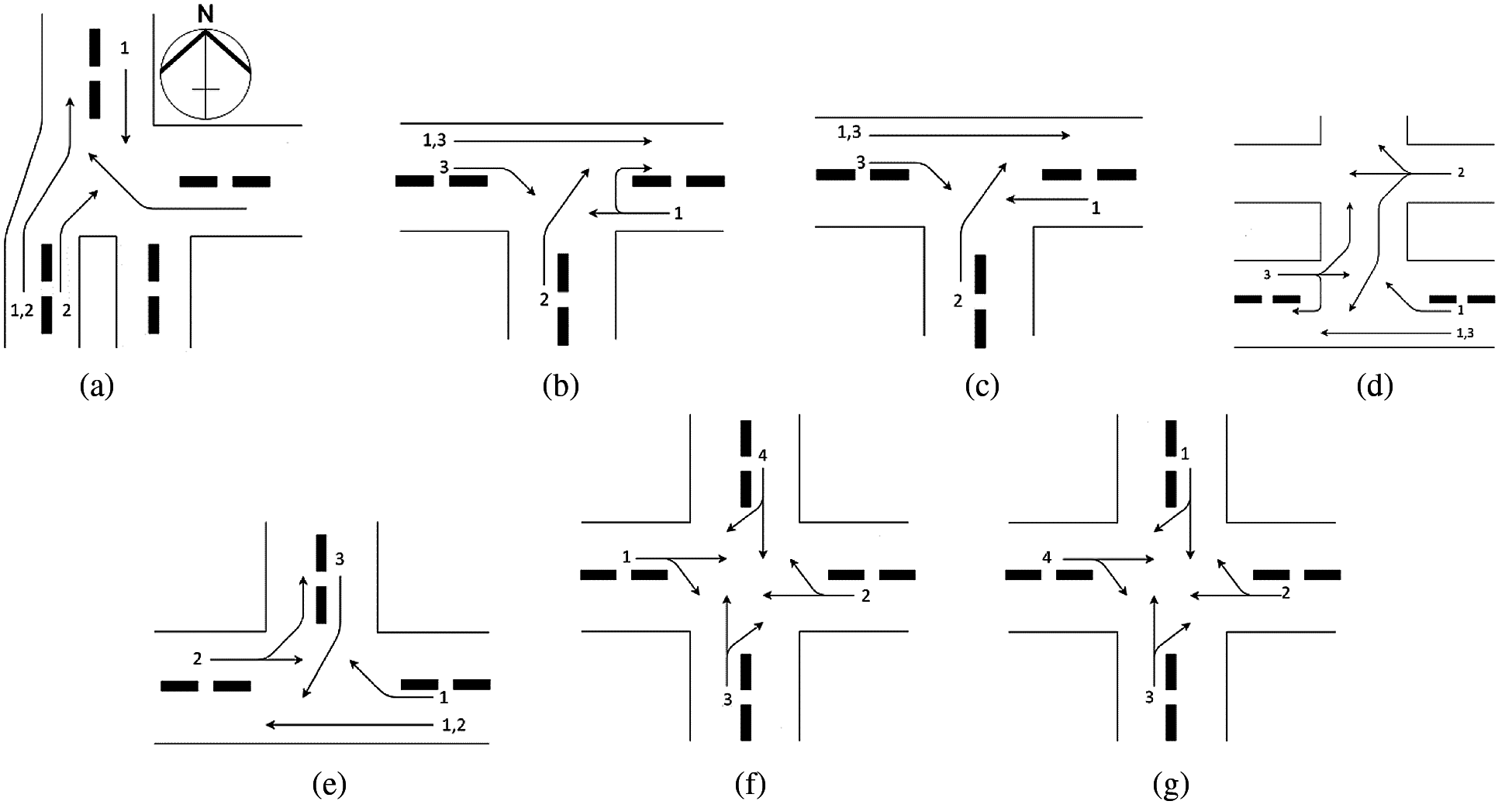
Figure 5: Seven intersections of the SCTN shown in Fig. 4. (a) Intersection 1 (b) Intersection 2 (c) Intersection 3 (d) Intersection 4 (e) Intersection 5 (f) Intersection 6 (g) Intersection 7
A GTN, which is a complex traffic network, has been widely adopted in the literature [15,44–47] to conduct similar investigations, and so it is selected for investigation in this paper to show that the proposed scheme is effective. This paper uses a 3 × 3 GTN with nine intersections, whereby a traffic light controller is installed at each intersection, which has 4 legs in four different directions (i.e., north bound, south bound, east bound, and west bound). Each leg has two lanes so that a vehicle can either enter or leave the leg of an intersection.
This subsection provides the specification of simulation setup. Two different traffic networks are investigated: a) SCTN with seven intersections (see Fig. 4), and b) a
5.4 Parameters of Simulation and Performance Measure
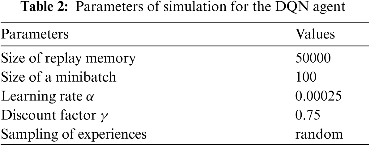
The parameters of simulation, which allow the best possible results for a DQN agent are presented in Tab. 2. Up to 50,000 experiences can be stored in a replay memory, and up to 100 experiences can be sampled randomly to form a minibatch. The values of parameters, which are presented in Tab. 2, have shown to provide the best possible performance in the literature [44].
Tab. 3 presents the parameters of simulation for the Burr type XII distribution model, which has various intensities of rainfall, including no rain (NR), light rain (LR), moderate rain (MR), and heavy rain (HR) scenarios [27]. The lower and higher scale parameter β value shrinks and stretches the distribution, respectively. The shape parameters
The performance measure used in this paper is the cumulative delay of the vehicles. Our proposed scheme aims to reduce the cumulative delay required by vehicles to cross multiple intersections. The cumulative delay also includes the average travelling and waiting times during congestion caused by RC and NRC. The total number of vehicles is 1000 per episode.
This section compares the performance measures achieved by our proposed MADQN, MARL and the baseline approaches, under RC and NRC traffic congestions. Fig. 6 presents a MADQN model loss during the training process under RC and NRC traffic congestions in SCTN and GTN. The lower model loss enhances the performances of both SCTN and GTN under both traffic congestions (i.e., RC and NRC).
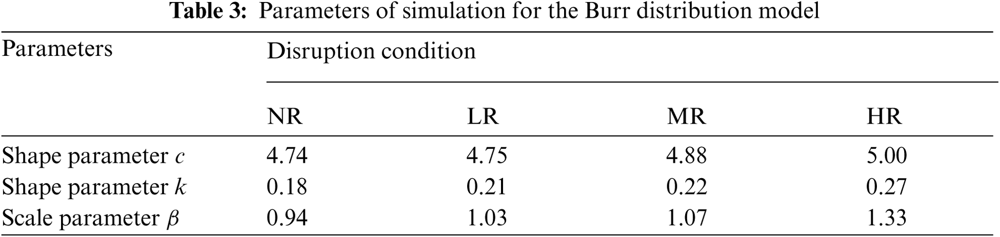
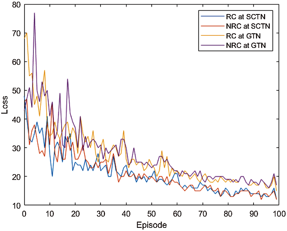
Figure 6: The MADQN model loss under RC and NRC traffic congestions in SCTN and GTN reduces with episode
5.5.1 Accumulated Delayed Reward
The accumulated delayed reward for MARL and MADQN under RC and NRC traffic congestions increases with episode in SCTN, as well as in GTN as shown in Fig. 7. The accumulated delayed reward for both MARL and MADQN approaches becomes steady after 50 episodes. As compared to MARL, the accumulated delayed reward achieved by MADQN is higher in both types of traffic congestions (i.e., RC and NRC) and traffic networks (i.e., SCTN and GTN). Overall, MADQN increases accumulated delayed reward by up to 10% and 12.5% under RC and NRC traffic congestions in the SCTN, and up to 8.3% and 7.2% under RC and NRC traffic congestions in the GTN, respectively.
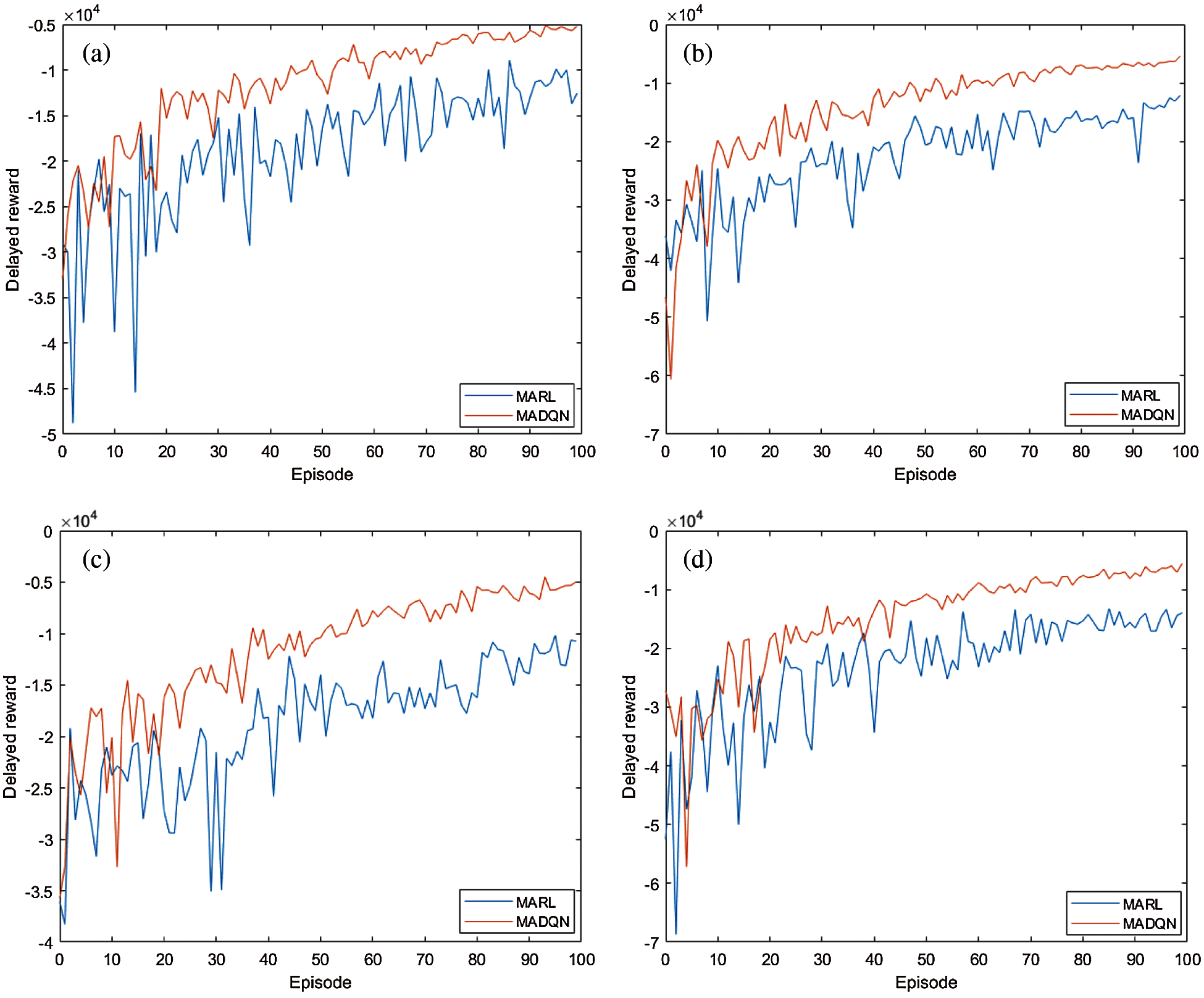
Figure 7: Accumulated delayed reward under RC and NRC traffic congestions in SCTN and GTN increases with episode. The accumulated delayed reward of MADQN is higher than that of MARL, which enhances the performances of both SCTN and GTN. (a) RC at SCTN (b) RC at GTN (c) NRC at SCTN (d) NRC at GTN
5.5.2 Cumulative Delay of the Vehicles
The cumulative delay of the vehicles for MADQN, MARL and the baseline approaches, under RC and NRC traffic congestions reduces with episode in SCTN as shown in Fig. 8. For both RC and NRC traffic congestions, MADQN outperforms MARL and the baseline approaches, in which MADQN achieves a lower cumulative delay compared to MARL and the baseline approaches under increased traffic volume. Similar trend is observed in GTN under RC and NRC traffic congestions as shown in Fig. 8. Overall, MADQN reduces cumulative delay of vehicles by up to 27.7% and 27.9% under RC and NRC traffic congestions in SCTN, and up to 28.5% and 27.8% under RC and NRC traffic congestions in GTN, respectively.
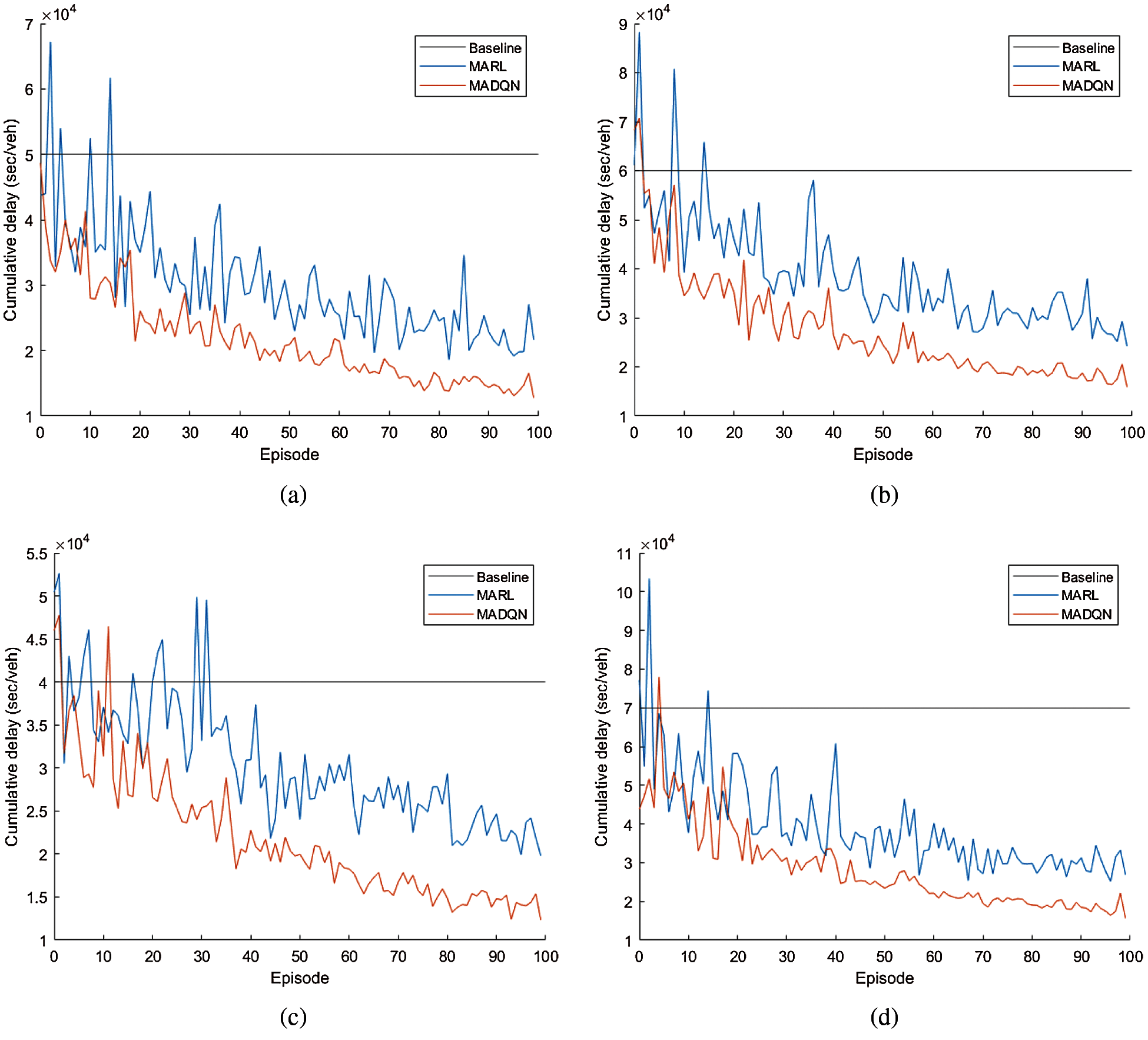
Figure 8: Cumulative delay of the vehicles under RC and NRC traffic congestions in SCTN and GTN reduces with episode. The cumulative delay of the baseline approach is fixed, and for the MARL and MADQN approaches, they reduce with episodes. MADQN has a lower cumulative delay than that of MARL and baseline approaches, which enhances the performances of both SCTN and GTN. (a) RC at SCTN (b) RC at GTN (c) NRC at SCTN (d) NRC at GTN
Fig. 9 presents a performance comparison between MARL and MADQN traffic light controllers in SCTN and GTN, in terms of cumulative delay of vehicles. MADQN achieves lower values compared to MARL in both SCTN and GTN under both RC and NRC traffic congestions. Overall, MADQN has similar results in RC and NRC traffic congestions because of its two main features, particularly target network and experience replay, which have shown outperforming results as compared to MARL in both complex GTN and real-world SCTN.
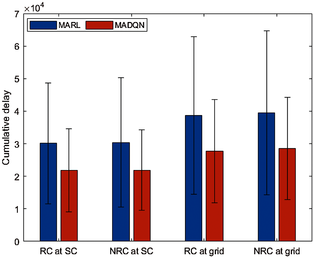
Figure 9: Performance comparison between MARL and MADQN traffic light controllers applied in SCTN and GTN under RC and NRC traffic congestions. MADQN achieves a lower cumulative delay compared to MARL under increased traffic volume. Lower cumulative delay enhances the performance of the traffic networks
6 Conclusions and Future Directions
This paper investigates the application of multi-agent deep Q-network (MADQN) to traffic light controllers at multiple intersections in order to address two types of traffic congestions: a) recurrent congestion (RC) caused by high volume of traffic; and b) non-recurrent congestion (NRC) caused by traffic disruptions, particularly bad weather conditions. From the traffic light controller perspective, MADQN adjusts traffic phase split according to traffic demand in order to minimize the number of waiting vehicles at different lanes of an intersection. From the MADQN perspective, it enables traffic light controllers to use deep neural networks (DNNs) to store and represent complex and continuous states, exchange knowledge (or Q-values), learn, and achieve optimal joint actions while addressing the curse of dimensionality in a multi-agent environment. There are two main features in MADQN, namely target network and experience replay, which provide training with stability in the presence of multiple traffic light controllers. MADQN is investigated in a traditional GTN and a real traffic network based on the Sunway city. Our simulation in Matlab and SUMO shows that MADQN outperforms MARL by reducing the cumulative delay of vehicles by up to
There are six future works that could be pursued to improve MADQN. Firstly, relaxing the assumption in which the left-turning (or right-turning) traffic movement is not protected or can conflict with other traffic movements in a left-hand (or right-hand) traffic network. Secondly, prioritizing the experiences during experience replay for faster learning in a multi-agent environment with multiple intersections. Thirdly, addressing the effects of dynamicity to MADQN, including the dynamic movement of vehicles. Fourthly, providing fairness and prioritized access among traffic flows at intersections. Fifthly, other kinds of disruptions of traffic, including crashes, could be considered into the state space as they tend to cause serious traffic congestion. Lastly, real field experiment can be conducted to train and validate the proposed scheme using real-world feedback. The real field data can be collected so that the traffic network and the system performance achieved in the simulation can be calibrated.
Funding Statement: This research was supported by Publication Fund under Research Creativity and Management Office, Universiti Sains Malaysia.
Conflicts of Interest: The authors declare that they have no conflicts of interest to report regarding the present study.
1. H. A. Aziz, F. Zhu and S. V. Ukkusuri, “Learning-based traffic signal control algorithms with neighborhood information sharing: An application for sustainable mobility,” Journal of Intelligent Transportation Systems, vol. 22, no. 1, pp. 40–52, 2018.
2. B. Yin, M. Dridi and A. El Moudni, “Traffic network micro-simulation model and control algorithm based on approximate dynamic programming,” IET Intelligent Transport Systems, vol. 10, no. 3, pp. 186–196, 2016.
3. S. B. Cools, C. Gershenson and B. D’Hooghe, “Self-organizing traffic lights: A realistic simulation,” in Advances in Applied Self-Organizing Systems. London: Springer, pp. 45–55, 2013.
4. J. C. Medina and R. F. Benekohal, “Traffic signal control using reinforcement learning and the max-plus algorithm as a coordinating strategy,” in 15th Int. IEEE Conf. on Intelligent Transportation Systems, Anchorage, AK, USA, pp. 596–601, 2012.
5. T. Semertzidis, K. Dimitropoulos, A. Koutsia and N. Grammalidis, “Video sensor network for real-time traffic monitoring and surveillance,” IET Intelligent Transport Systems, vol. 4, no. 2, pp. 103–112, 2010.
6. S. El-Tantawy, B. Abdulhai and H. Abdelgawad, “Multiagent reinforcement learning for integrated network of adaptive traffic signal controllers (MARLIN-ATSCMethodology and large-scale application on downtown Toronto,” IEEE Transactions on Intelligent Transportation Systems, vol. 14, no. 3, pp. 1140–1150, 2013.
7. S. Shen, G. Shen, Y. Shen, D. Liu, X. Yang et al., “PGA: An efficient adaptive traffic signal timing optimization scheme using actor-critic reinforcement learning algorithm,” KSII Transactions on Internet and Information Systems (TIIS), vol. 14, no. 11, pp. 4268–4289, 2020.
8. C. T. Phan, D. D. Pham, H. V. Tran, T. V. Tran and P. N. Huu, “Applying the IoT platform and green wave theory to control intelligent traffic lights system for urban areas in Vietnam,” KSII Transactions on Internet and Information Systems (TIIS), vol. 13, no. 1, pp. 34–51, 2019.
9. F. Rasheed, K. L. A. Yau, R. M. Noor, C. Wu and Y. C. Low, “Deep reinforcement learning for traffic signal control: A review,” IEEE Access, vol. 8, pp. 208016–208044, 2020.
10. R. S. Sutton and A. G. Barto, Reinforcement Learning: An Introduction, 2nd ed., Cambridge: The MIT Press, 2018.
11. M. F. Khan and K. L. A. Yau, “Route selection in 5G-based flying ad-hoc networks using reinforcement learning,” in 10th IEEE Int. Conf. on Control System, Computing and Engineering (ICCSCEPenang, Malaysia, pp. 23–28, 2020.
12. L. Buşoniu, R. Babuška and B. De Schutter, “Multi-agent reinforcement learning: An overview,” in Innovations in Multi-Agent Systems and Applications. Berlin, Heidelberg: Springer, pp. 183–221, 2010.
13. K. L. A. Yau, J. Qadir, H. L. Khoo, M. H. Ling and P. Komisarczuk, “A survey on reinforcement learning models and algorithms for traffic signal control,” ACM Computing Surveys (CSUR), vol. 50, no. 3, pp. 1–38, 2017.
14. V. Mnih, K. Kavukcuoglu, D. Silver, A. A. Rusu, J. Veness et al., “Human-level control through deep reinforcement learning,” Nature, vol. 518, no. 7540, pp. 529–533, 2015.
15. F. Rasheed, K. L. A. Yau and Y. C. Low, “Deep reinforcement learning for traffic signal control under disturbances: A case study on Sunway city, Malaysia,” Future Generation Computer Systems, vol. 109, no. 3, pp. 431–445, 2020.
16. Y. LeCun, Y. Bengio and G. Hinton, “Deep learning,” Nature, vol. 521, no. 7553, pp. 436–444, 2015.
17. V. Mnih, K. Kavukcuoglu, D. Silver, A. Graves, I. Antonoglou et al., “Playing Atari with deep reinforcement learning,” arXiv preprint arXiv:1312.5602, 2013.
18. M. Gregurić, K. Kušić, F. Vrbanić and E. Ivanjko, “Variable speed limit control based on deep reinforcement learning: A possible implementation,” in Int. IEEE Symp. ELMAR, Zadar, Croatia, pp. 67–72, 2020.
19. Clarivate Analytics, Web of science. [Online]. Available: https://www.webofknowledge.com.
20. IEEE, IEEE Xplore. [Online]. Available: https://ieeexplore.ieee.org.
21. Elsevier, ScienceDirect. 1997. [Online]. Available: https://www.sciencedirect.com.
22. W. Genders and S. N. Razavi, “Using a deep reinforcement learning agent for traffic signal control,” arXiv: 1611.01142, 2016.
23. S. S. Mousavi, M. Schukat and E. Howley, “Traffic light control using deep policy-gradient and value-function-based reinforcement learning,” IET Intelligent Transport Systems, vol. 11, no. 7, pp. 417–423, 2017.
24. B. Anbaroğlu, T. Cheng and B. Heydecker, “Non-recurrent traffic congestion detection on heterogeneous urban road networks,” Transportmetrica A: Transport Science, vol. 11, no. 9, pp. 754–771, 2015.
25. A. Skabardonis, P. Varaiya and K. F. Petty, “Measuring recurrent and nonrecurrent traffic congestion,” Transportation Research Record, vol. 1856, no. 1, pp. 118–124, 2003.
26. W. F. Adams, “Road traffic considered as a random series,” Journal of the Institution of Civil Engineers, vol. 4, no. 1, pp. 121–130, 1936.
27. H. M. Alhassan and J. Ben-Edigbe, “Effect of rain on probability distributions fitted to vehicle time headways,” International Journal on Advanced Science, Engineering and Information Technology, vol. 2, no. 2, pp. 31–37, 2012.
28. S. Krauß, P. Wagner and C. Gawron, “Metastable states in a microscopic model of traffic flow,” Physical Review E, vol. 55, no. 5, pp. 5597–5602, 1997.
29. M. Gregurić, M. Vujić, C. Alexopoulos and M. Miletić, “Application of deep reinforcement learning in traffic signal control: An overview and impact of open traffic data,” Applied Sciences, vol. 10, no. 11, pp. 4011, 2020.
30. I. Goodfellow, Y. Bengio and A. Courville, Deep Learning. Cambridge: MIT press, 2016.
31. J. Fan, Z. Wang, Y. Xie and Z. Yang, “A theoretical analysis of deep Q-learning,” in Learning for Dynamics and Control, virtual conference, pp. 486–489, 2020.
32. M. Tan, “Multi-agent reinforcement learning: independent vs. cooperative agents,” in Proc. of the 10th Int. Conf. on Machine Learning, Amherst, MA, USA, pp. 330–337, 1993.
33. C. H. Wan and M. C. Hwang, “Value-based deep reinforcement learning for adaptive isolated intersection signal control,” IET Intelligent Transport Systems, vol. 12, no. 9, pp. 1005–1010, 2018.
34. J. Gao, Y. Shen, J. Liu, M. Ito and N. Shiratori, “Adaptive traffic signal control: Deep reinforcement learning algorithm with experience replay and target network,” arXiv preprint arXiv: 1705.02755, 2017.
35. K. L. Tan, S. Poddar, S. Sarkar and A. Sharma, “Deep reinforcement learning for adaptive traffic signal control,” in Dynamic Systems and Control Conf., American Society of Mechanical Engineers, Utah, USA, 2019.
36. H. Wei, G. Zheng, H. Yao and Z. Li, “Intellilight: A reinforcement learning approach for intelligent traffic light control,” in Proc. of the 24th ACM SIGKDD Int. Conf. on Knowledge Discovery & Data Mining, London, UK, pp. 2496–2505, 2018.
37. L. Li, Y. Lv and F. Y. Wang, “Traffic signal timing via deep reinforcement learning,” IEEE/CAA Journal of Automatica Sinica, vol. 3, no. 3, pp. 247–254, 2016.
38. T. Chu, J. Wang, L. Codecà and Z. Li, “Multi-agent deep reinforcement learning for large-scale traffic signal control,” IEEE Transactions on Intelligent Transportation Systems, vol. 21, no. 3, pp. 1086–1095, 2019.
39. T. T. Nguyen, N. D. Nguyen and S. Nahavandi, “Deep reinforcement learning for multiagent systems: A review of challenges, solutions, and applications,” IEEE Transactions on Cybernetics, vol. 50, no. 9, pp. 3826–3839, 2020.
40. K. L. A. Yau, S. L. Lau, H. N. Chua, M. H. Ling et al., “Greater Kuala Lumpur as a smart city: A case study on technology opportunities,” in 8th Int. Conf. on Knowledge and Smart Technology (KSTChiangmai, Thailand, pp. 96–101, 2016.
41. A. R. Syakura, M. Z. A. Ab Kadir, C. Gomes, A. B. Elistina and M. A. Cooper, “Comparative study on lightning fatality rate in Malaysia between 2008 and 2017,” in 34th Int. Conf. on Lightning Protection (ICLPRzeszow, Poland, pp. 1–6, 2018.
42. N. Krishnan, M. V. Prasanna and H. Vijith, “Fluctuations in monthly and annual rainfall trend in the limbang river basin, Malaysia: a statistical assessment to detect the influence of climate change,” Journal of Climate Change, vol. 4, no. 2, pp. 15–29, 2018.
43. M. Behrisch, L. Bieker, J. Erdmann and D. Krajzewicz, “SUMO-simulation of urban mobility: An overview,” in Proc. of SIMUL 2011, The Third Int. Conf. on Advances in System Simulation, ThinkMind, Barcelona, Spain, 2011.
44. E. van der Pol and F. A. Oliehoek, “Coordinated deep reinforcement learners for traffic light control,” in Proc. of 30th Conf. Neural Inf. Process. Syst., no. Nips, Barcelona, Spain, pp. 8, 2016.
45. L. A. Prashanth and S. Bhatnagar, “Threshold tuning using stochastic optimization for graded signal control,” IEEE Transactions on Vehicular Technology, vol. 61, no. 9, pp. 3865–3880, 2012.
46. M. A. Khamis, W. Gomaa and H. El-Shishiny, “Multi-objective traffic light control system based on Bayesian probability interpretation,” in 15th Int. IEEE Conf. on Intelligent Transportation Systems, Anchorage, USA, pp. 995–1000, 2012.
47. T. Chu, J. Wang, L. Codecà and Z. Li, “Multi-agent deep reinforcement learning for large-scale traffic signal control,” IEEE Transactions on Intelligent Transportation Systems, vol. 21, no. 3, pp. 1086–1095, 2019.
48. D. J. Higham and N. J. Higham, MATLAB Guide. Philadelphia, PA, USA: SIAM, 2016.
49. A. F. Acosta, J. E. Espinosa and J. Espinosa, “TraCI4Matlab: Enabling the integration of the SUMO road traffic simulator and Matlab® through a software re-engineering process,” in Modeling Mobility with Open Data, Cham: Springer, pp. 155–170, 2015.
 | This work is licensed under a Creative Commons Attribution 4.0 International License, which permits unrestricted use, distribution, and reproduction in any medium, provided the original work is properly cited. |