Computers, Materials & Continua DOI:10.32604/cmc.2022.022018
Article

Optimization of Interval Type-2 Fuzzy Logic System Using Grasshopper Optimization Algorithm

Saima Hassan1, Mojtaba Ahmadieh Khanesar2, Nazar Kalaf Hussein3, Samir Brahim Belhaouari4,*, Usman Amjad5 and Wali Khan Mashwani6

1Institute of Computing, Kohat University of Science and Technology, Kohat, Pakistan
2Department of Mechanical, Materials and Manufacturing Engineering, Faculty of Engineering, University of Nottingham, UK
3College of Computer Sciences and Mathematics, Tikrit University, Iraq
4Division of Information and Computing Technology, College of Science and Engineering, Hamad Bin Khalifa University, Qatar
5Department of Computer Science, Sir Syed University of Engineering and Technology, Pakistan
6Institute of Numerical Sciences, Kohat University of Science and Technology, Kohat, Pakistan
*Corresponding Author: Samir Brahim Belhaouari. Email: sbelhaouari@hbku.edu.qa
Received: 24 July 2021; Accepted: 06 October 2021

Abstract: The estimation of the fuzzy membership function parameters for interval type 2 fuzzy logic system (IT2-FLS) is a challenging task in the presence of uncertainty and imprecision. Grasshopper optimization algorithm (GOA) is a fresh population based meta-heuristic algorithm that mimics the swarming behavior of grasshoppers in nature, which has good convergence ability towards optima. The main objective of this paper is to apply GOA to estimate the optimal parameters of the Gaussian membership function in an IT2-FLS. The antecedent part parameters (Gaussian membership function parameters) are encoded as a population of artificial swarm of grasshoppers and optimized using its algorithm. Tuning of the consequent part parameters are accomplished using extreme learning machine. The optimized IT2-FLS (GOAIT2FELM) obtained the optimal premise parameters based on tuned consequent part parameters and is then applied on the Australian national electricity market data for the forecasting of electricity loads and prices. The forecasting performance of the proposed model is compared with other population-based optimized IT2-FLS including genetic algorithm and artificial bee colony optimization algorithm. Analysis of the performance, on the same data-sets, reveals that the proposed GOAIT2FELM could be a better approach for improving the accuracy of the IT2-FLS as compared to other variants of the optimized IT2-FLS.

Keywords: Parameter optimization; grasshopper optimization algorithm; interval type-2 fuzzy logic system; extreme learning machine; electricity market forecasting

1  Introduction

The ability of processing noisy and uncertain data has made the use of fuzzy sets in numerous applications a vital option. One such application is the fuzzy logic system (FLS) that is solving prediction, classification and control problems effectively. Initial version of the FLS, known as type-1 fuzzy logic system (T1-FLS), is based on fuzzy set that has crisp membership values. Modification and extension to the fuzzy sets were mainly studied over the past few decades. These include interval-valued fuzzy set [1], general Type-2 fuzzy set [2] and interval T2-fuzzy set [3]. Type-2 fuzzy logic system (T2-FLS) with the presence of footprint-of uncertainty can model and handle the uncertainty very well [4]. However, current research of the T2-FLS has been dominated by the research applications of IT2-FLS, due to its simpler structure and reduced computational cost, as compared to a general T2-FLS [4]. Fuzzy membership functions like Gaussian, triangular and trapezoidal are used to define a fuzzy set. Every membership function has its own parameters to be selected for defining fuzzy rules. T1-FLSs use crisp values of these parameter, however, using an exact membership value for may not be the best way to deal with uncertainty in data. A T2-FLS with fuzzy membership functions can handle any type of uncertainty by the concept of blurring a T1 membership function. However, this blurring approach to form a secondary membership, the third dimension, in T2-FLS is a complex and computationally expensive task. Instead of fuzzy or blur membership, IT2-FLS uses interval values for membership function parameters, ignoring the third dimension of the T2-FLS, that eventually simplifies the computation. The rules (If-then parts), shape and operators are different components of a FLS that is described as the fuzzy system's parameters. Learning of these parameter is needed to be adaptively constructed in order to handle the prevailing uncertainties and imprecision of nonlinear dynamic systems. Among various approaches to handling uncertain data, it is observed that most studies on IT2-FLSs are confronted with determining the optimal parameters [5].

Generally, both premise part and consequent part of a FLS can be optimized, however; optimization of the parameters of a fuzzy inference has attracted much attention of the research community [5]. Fuzzy inference system (FIS) consists of if-then rules that represent the antecedent part (AP) and the consequent part (CP), respectively. Artificial neural networks being the simplest method has been utilized to determine the FIS [6], however, such neuro-fuzzy model does not guarantee the convergence and/or effectiveness of the optimal FIS. In order to tackle this issue, optimization of the FIS was tackled by incorporating the population information of the evolutionary algorithms [7]. T1 and T2-FLS have a history to be optimized with various population based optimization algorithms, for example, some of the recent work of these optimization algorithms can be found in [8–10]. Likewise, appropriate parameters and structure of the IT2-FLS can also be optimized using different optimization algorithms. A general framework for the design of IT2-Fuzzy controllers based on various bio-inspired algorithms was presented in [11]. A concise review of bio-inspired algorithms namely particle swarm optimization (PSO), genetic algorithm (GA) and Ant colony optimization to tune IT2-FLS parameters for different applications can be found in [12]. Optimization of an IT2-FLS has also been carried out using artificial bee colony (ABC) optimization [13], PSO [14], and Cuckoo search algorithm [15]. A comparative analysis of two optimized IT2-FLS with the randomly and manually generated parameters of IT2-FLS was presented in [16] with noise-free and noisy Mackey-glass time series prediction. The results revealed better performance of the optimized IT2-FLS with noisy dataset as compared to other approaches. Grasshopper optimization algorithm (GOA) is a newly proposed [17] population based meta-heuristic algorithm that mimics the swarming behavior of grasshoppers in nature. The main feature of GOA is the movement of swarm, which is defined based on the position of all individual grasshoppers in the swarm. GOA for various optimization problems has shown its efficiency as compared to existing optimization algorithms. A GOA based parameter optimized PI controller has proved its enhanced performance over PSO and Whale optimization algorithm based controller [18]. Kernel function and penalty factor of a support vector machine (SVM) was optimized using GOA and was evaluated for a regional power load forecasting [19].

Our previous works presenting hybrid intelligent approaches to tune the parameters of IT2-FLSs are hybrid of ABC and extreme learning machine (ELM) [13] and hybrid of GA and ELM [16]. Hybrid methods demonstrate superior performance as an intelligent optimizer is used for AP and a computational approach is utilized to train the linear parameters. Use of hybrid methods makes it possible to skip local minima which naturally exist when optimizing the AP. Hybrid algorithms have already shown their superior priority over several other state-of-the-art optimization algorithms in literature including PSO [20], discrete heuristic particle swarm ant colony optimization [21], mine blast algorithm [22], and symbiotic organisms search [23]. The probability of this heuristic approach to deal with local minima is investigated in different benchmark optimization problems including convex optimization problems, non-convex optimization problems, and the ones with several local minima [17]. The superior performance of the GOA over other optimization algorithm has motivated us to propose a new variant of our previous work, where the Gaussian membership function parameters are optimized using GOA for the electricity load and price forecasting.

This paper presents hybrid of GOA and ELM to tune the parameters of the IT2-FLS. The GOA is for the first time used to optimize the APs of an IT2-FLS. Optimization of the CPs using ELM (IT2FELM) can be seen in [24] with random generated APs. This research work is the continuation of our previous work [13], where GA and ABC were utilized for the parameter optimization of the IT2FELM.

The structure of the rest of this paper is as follows. The background studies of the methods used is given in Section 2. Methodology of the proposed hybrid learning algorithm is presented in Section 3. Data and results are discussed in Section 4. The paper is concluded with some remarks and recommendation in Section 5.

2  Preliminaries

This section defines IT2-FLS including some relevant concepts along well defined mathematics are provided so as to report these sets in an effectual manner. In order to begin, the taxonomy of T1 fuzzy set followed by T2 fuzzy set expressed mathematically so as to facilitate the discussion of this article.

Definition 1. IF X≠0 is a collection of objects denoted generically by x, then a fuzzy set F in X is defined as F={(x,μF(X))|x∈X}. μF:X→[0,1] is the membership function (MF) and the degree of membership of x in F is μF(x), ∀x∈X [25].

Definition 2. A type-2 fuzzy set, denoted by F~ is characterized by a type-2 membership function μF~(x,u), where x∈X and u∈Jx⊂[0,1] , i.e.,

F~=((x,u),μF~(x,u))|∀x∈X,∀u∈Jx⊆[0,1](1)

in which μF~(x,u)∈[0,1]. When X×Jx is continuous then F~ can be expressed as

F~=∫x∈X⁡∫u∈J⁡μF~(x,u)/(x,u)Jx⊆[0,1],(2)

where ∫⁡∫ denotes union over all admissible x and u.

Jx is known as the primary MF of x in F~. At each value of x say x=x′, the two-dimensional plane, whose axes are u and μF~(x′,u), is called a vertical slice of μF~(x,u) [26]. A secondary MF is a vertical slice of μF~(x,u). It is μF~(x=x′,u) for x′∈X and ∀u∈Jx′⊆[0,1], i.e.,

μF~(x=x′,u)≡μF~(x′)=∫u∈Jx′⁡1/uJx′⊆[0,1](3)

Because ∀x′∈X, the prime notation on μF~(x′) can be referred to μF~(x) as a secondary set [26].

Definition 3. The Interval Type-2 (IT2) Fuzzy Sets F~ is a special case of T2 fuzzy set. A T2 fuzzy set with a uniform secondary MF is called an IT2 fuzzy set, i.e., μF~(x,u)=1 for all x∈X. IT2 fuzzy set in accordance to Eq. (2) can be expressed as

F~=∫x∈X⁡∫u∈J⁡1/(x,u)Jx⊆[0,1](4)

The uncertainty in the IT2 fuzzy set due to the presence of an upper MF and lower MF called the footprints of uncertainty (FOUs) and are denoted by μ¯F~(x) and μ_F~(x) (e.g., see Fig. 1b). It is the Union of all primary MFs.

Figure 1: Illustration of fuzzy membership functions (a) Type-1 fuzzy membership function (b) interval type-2 fuzzy membership function

2.1 Interval Type-2 Fuzzy Logic System

The idea of Fuzzy Set Theory was given by Zadeh [27] to cater the ambiguities and uncertainties present in real world problems. Elements belong to a set based on the MF which gives real values in interval [0,1]. Since the introduction, fuzzy sets faced criticism that MF used in traditional or T1 fuzzy set are not fuzzy numbers so there is no uncertainty in that and thus opposing the concept of fuzzy logic. To address the issue Zadeh [25] proposed another type of fuzzy sets which he called T2 fuzzy set. A T2 fuzzy set handles this issue by incorporating fuzziness or uncertainty in the MF. A T2 fuzzy set has a MF which is fuzzy and has three dimensions. Membership of each element of this fuzzy set is itself another fuzzy set in the range [0,1]. This third dimension in T2 fuzzy set provides extra degree of freedom to cater additional information about the value. These fuzzy sets are used when it becomes difficult to find out exact MF of a fuzzy set. The IT2-FLS are computationally less expensive as compared to general T2-FLS as the secondary MF of IT2 MF is equal to 1. The structure of an IT2-FLS is given in Fig. 2.

Figure 2: Structure of interval type-2 fuzzy logic system

The fuzzifier in an IT2-FLS maps an input vector x=[x1,x2,⋯,xd]T into d IT2 fuzzy sets F~i,i=1,2,⋯,d. In order to choose the type of MF, Gaussian MF is preferred as it cover the entire input domain and hence guarantee continuity during the input-output mapping. A Gaussian MF with a fixed mean min and uncertain standard deviation [σin1,σin2 is considered here [5]:

μF~in(xi)=exp[−12(xi−minσin)2],σin∈[σin1,σin2],(5)

where mean and spread of the Gaussian MF are represented by min,σin, respectively. μF~in(xi) of Eq. (5) has upper MF, μ¯F~in(xi), and lower MF, μ_F~in(xi), as follows:

μ¯F~in(xi)=N(min,σin2;xi)(6)

μ_F~in(xi)=N(min,σin1;xi)(7)

A TSK fuzzy rule (Rn) in the rule set with N rules of an IT2-FLS can be expressed as [25]:

Rn: IF x1 is F~1n∧x2 is F~2n∧⋯∧xd is F~dn THEN yn(x)=[y_n,y¯n]

where y_n,y¯n,c_in and c¯in are crisp numbers. The total firing interval Fn=[f_n,f¯n] of the IT2 fuzzy set is described as:

f_n(x)=μ_F~1n(x1)⋆μ_F~2n(x2)⋆⋯⋆μ_F~dn(xd)=∏i=1d⁡μ_F~in(xi)(8)

and

f¯n(x)=μ¯F~1n(x1)⋆μ¯F~2n(x2)⋆⋯⋆μ¯F~dn(xd)=∏i=1d⁡μ¯F~in(xi)(9)

The output of the THEN-part (consequent part) of the nth rule is a crisp value that can be written as:

y_n=y¯n=c0n+c1nx1+⋯+cdnxd,=∑i=0d⁡cinxi=yn,x0=Δ1.(10)

The output sets received from the rule firing interval Fn(x) and the corresponding rule consequents Y=[yl,yr] are IT2 fuzzy sets. A Type reducer computes the IT2 fuzzy sets using

Y=[yl,yr]=∫y1∈[y_1,y¯1]⁡⋯∫yN∈[y_1,y¯1]⁡∫f1∈[f_1,f¯1]⁡⋯∫fN∈[f_N,f¯N]⁡1∑n=1N⁡fnyn∑n=1N⁡fn.(11)

The Karnik-Mendel (K-M) algorithm [28] as a centroid type reduction is used to obtain T1 fuzzy sets. Finally, the crisp output for each output variable can be obtained during defuzzification as:

y=(yl+yr)2.(12)

2.2 Grasshopper Optimization Algorithm (GOA)

The Grasshopper Optimization Algorithm (GOA) is a modern steepest meta-heuristic optimization algorithm based on natural swarms of grasshoppers. The two aspects of any metaheuristic algorithm are exploration in which the agents freely move to explore the search space and exploitation where the neighborhood is exploited to reach optimal solution [17,29]. The basic inspiration of GOA mimics two concepts of grasshopper swarm; the first is the slow motion of grasshopper larvae swarms in order to find the food and exploit the region fully, the second is the adult grasshoppers which move quickly and suddenly by individuals or swarms to explore to find new places contains food. The principles of exploration and exploitation are thus implemented in GOA in this way. The mathematic model of GOA is described below: If the current position of the ith grasshopper in swarm is represented by Xi, the social interaction of ith grasshopper as Si, the gravity force on ith grasshopper as Gi and the wind advection as Ai than

Xi=Si+Gi+Ai(13)

The social interaction between the ith grasshopper and jth grasshopper with the Euclidian distance dij=|xj−xi| in Eq. (13) is calculated as:

Si=∑j=1j≠iN⁡s(dij)d→iji≠j(14)

where d→ijxj−xidij represents a unit vector for distance between ith and jth grasshopper. The strength of social forces s with intensity of attraction f and attractive length scale l is calculated as a function as follows

s(r)=fe−dl−e−d(15)

Similarly, the gravity component G of Eq. (13) with the gravitational constant g and a unity vector towards the center of earth e→g is computed as:

Gi=−ge→g(16)

The last component wind direction Ai in Eq. (13) with a constant drift u and a unity vector in the direction of wind e→w is calculated as follows

Ai=−ue→w(17)

Substituting Eqs. (14), (16) and (17) in (13) the extended form of Xi is obtained as follows

Xi=−∑j=1j≠iN⁡|xj−xi|xj−xidij−ge→g+ue→w(18)

Since various grasshoppers reach the comfort zone very soon and contribute less towards optimization so the Eq. (18) cannot be used directly. To solve the issue of optimization for comprehensive convergence, i.e., the arrival of grasshopper flock to the goal and converge there in the target area, the previous equation can be modified as

Xi=c[∑j=1j≠iN⁡cubd−lbddijs(xj−xi)xj−xidij]+Td,(19)

where ubd, lbd are the upper and lower bound and Td is the target value in the dth dimension. The parameter c is called a decreasing coefficient and it is responsible for reducing the comfort zone, repulsion zone and the attraction zone. c it is calculated as follow

c=cmax−lcmax−cminL,(20)

where l is the current iteration, cmax, cmin are the maximum and minimum value which are assume in the begining and the L is the maximum number of iterations. It is evident from Eq. (19) that for every grasshopper agent the next position is determined by using the current position of agent along with target position and other agents’ positions. Eq. (19) also shows that the first component takes into account the position of current agent with respect to other agent. Moreover, the positions of all agents are taken into account for defining positions of search agents around the target.

2.3 Extreme Learning Machine (ELM)

ELM as a tuning-free algorithm for SLFN was proposed in [30], where the input weights and hidden biases are chose randomly. Brief mathematics of ELM for SLFNs is described as follows.

Given an arbitrary D training samples (xi,yi)i=1D, where xi=[xi1,xi2.⋯,xid]⊂Rd and yi=[yi1,yi2,⋯,yim]⊂Rm, the output of an SLFNs with N~ hidden nodes and G(x) activation function is modeled as:

∑j=1N~⁡βj,kGj(xi)=∑j=1N~⁡βjG(xi;wj,bj)=yi,k,i=1,…,Dandk=1,…,m,(21)

where wi and bi are parameters of the activation function G(xj;wi,bi). Eq. (21) in a matrix form can be rewritten as:

Hβ=Y(22)

where

  =[ G(x1;w1,b1)amp;⋯amp;G(x1;wN˜,bN˜)⋮amp;⋱amp;⋮G(xD;w1,b1)amp;⋯amp;G(xD;wN˜,bN˜) ]D×N˜(23)

β=[β1T⋮βN~T]N~×m=[β11⋯β1m⋯⋱⋯βN~1⋯βN~m]N~×m(24)

and

Y=[y1T⋮yDT]D×m(25)

Here H is known as the hidden layer output matrix generated randomly with parameters wi and bi. βi is the output weight matrix, yT is the transpose of vector y. An optimal solution β^ of βi under the constraint of minimum least square minβ∥β∥ and minβ∥Hβ−Y∥ of the linear system in Eq. (22) can be calculated as

β^=H†Y(26)

where H† is the Moore-Penrose generalized inverse of matrix H [31].

3  Methodology of the Hybrid Learning Algorithm (GOAIT2FELM)

The AP parameters appear nonlinearly in the output and the CP parameters appear linearly. The problem which is addressed in this paper involves the training of IT2-FLS parameters using hybrid of GOA and ELM. The proposed hybrid learning algorithm tune the CPs using ELM with randomly generated APs initially. The APs are then encoded in a population of artificial swarm and optimized using GOA in the direction of having best candidate solution. Fig. 3 shows the flowchart of the design of IT2-FLS using hybrid learning algorithm of GOA and ELM. As can be seen from the flowchart, the proposed estimation method is mainly an iterative approach in which the parameters which appear non-linearly in the CP are trained using GOA and the linear parameters are trained using ELM.

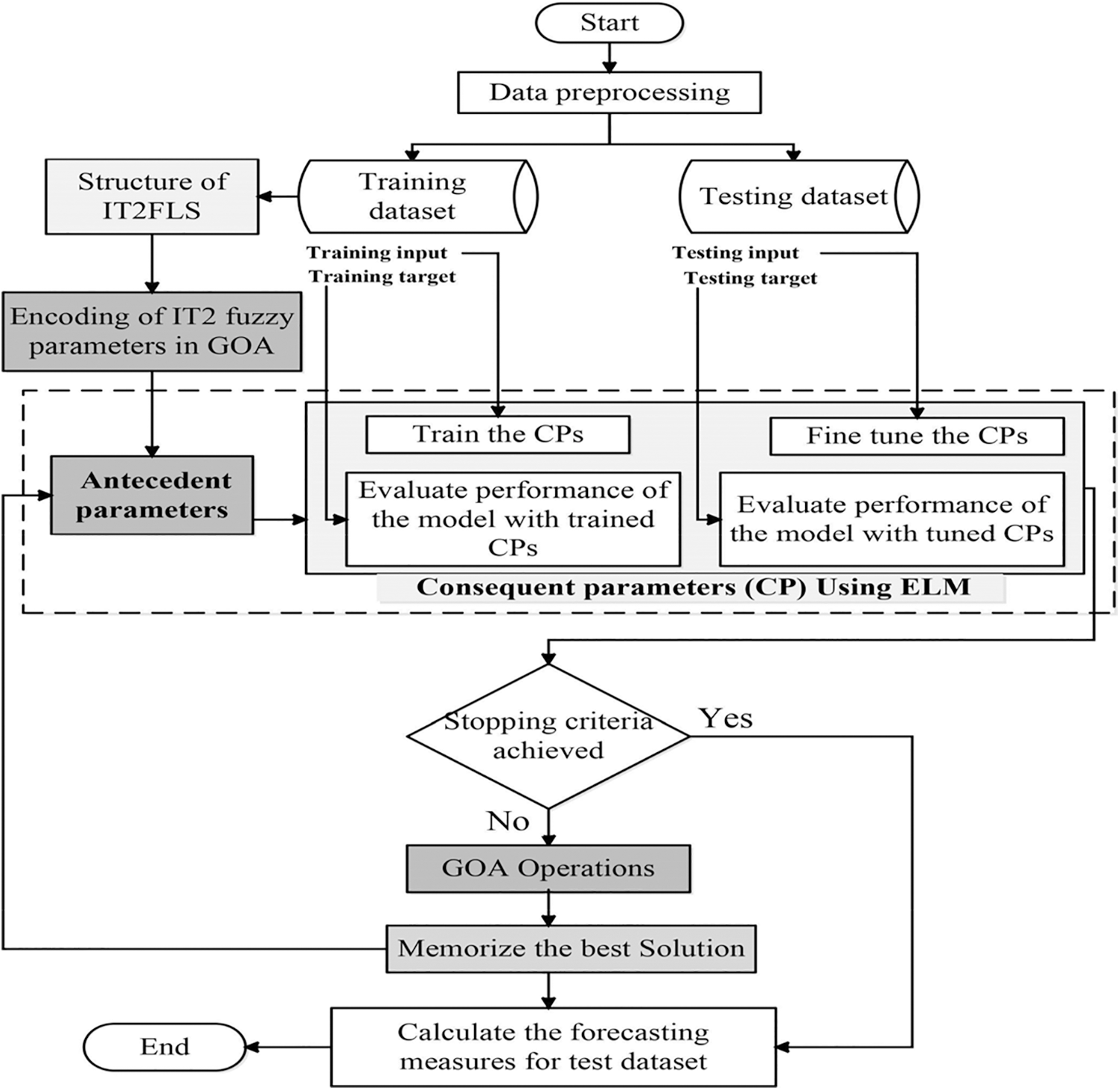
Figure 3: Flowchart of the proposed model

3.1 Data Preprocessing and Input Selection

The data pre-processing techniques reduces the complexity in data, and will enable the Proposed models trained with this data to exhibit better predictive performance. Data is normalized in a range between [0,1] using the following equation

DN=Di−DminDmax−Dmin,(27)

where DN represents the normalized data. The data sets used are divided into two sets of training and testing. Training data set is used during the training of proposed model whereas the model performance is evaluated with the testing data set. The proposed model utilizes multi-inputs to the system. A partial autocorrelation analysis is utilized as input-selection method, that selects the influential inputs for a model. The time-delays of the data set which have significant coefficients are selected as inputs to the model.

3.2 Structure of the Interval Type-2 Fuzzy Logic System

The hybrid learning algorithm is proposed for a TSK based IT2-FLS. The IT2-FLS described in Section 2.1, also known as A2-C1, is utilized here to approximate the input-output relationship of the problem. Here “A” and “C” are short for antecedent and consequent, respectively. This indicates that the Aps of this IT2-FLS are T2FSs and the CP are T1FSs.

3.3 Antecedent Parameter Generation Using GOA

The IT2 Gaussian MF with uncertain standard deviation [σin1,σin2] and fixed mean min are the parameters that need to be learnt using GOA. Therefore, these APs are encoded into a swarm of artificial grasshopper and computed using Eqs. (13), (14), (16) and (17). While learning any fuzzy system, encoding of the parameters into corresponding optimization algorithm is the main task. The APs here are encoded as the population of grasshopper. Let Xi=[xi1,xi2,⋯,xiM](i=1,2,⋯,P), represents the ith grasshopper in the population. Then Xi can be initialized randomly as:

Xi=rand(d×M×3)(28)

where P, d and M are the population size, number of inputs and number of membership functions, respectively. Considering the three parameters of the IT2 Gaussian MF, the total length of the solution size becomes d×M×3. Encoding of the IT2 fuzzy APs into a population of grasshopper in a vector form is represented in Eq. (29) and is illustrated in Fig. 4 as follows:

F=[m11,⋯,mMd,σ111,⋯,σ1Md,σ211,⋯,σ2Md](29)

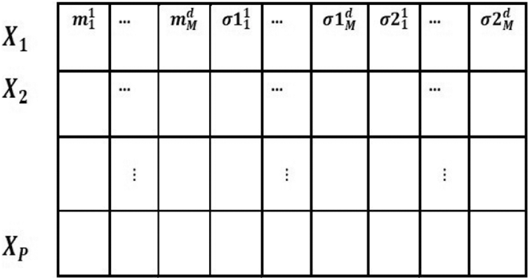
Figure 4: Encoding of antecedent parameters into a swarm

3.4 Consequent Parameter Tuning Using ELM

In order to determine rule consequent in the hybrid algorithm GOA-ELM, ELM is employed as in [24,32]. Setting and tunning of the CPs are done accordingly as our previous work [24].

3.5 Cost Function

With the aim of learning the APs of the IT2-FLS, fitness of the individual grasshopper population is evaluated with a cost function in the hybrid learning algorithm. Lower the value of the cost function higher will be the fitness of the candidate solution. Individual swarm of grasshopper produces a modification on the IT2 fuzzy Aps in each iteration and evaluate it with the RMSE (Eq. (31)) as a cost function.

3.6 Verification

In order to verify, performance of the proposed hybrid learning algorithm, test data-set is used and evaluated with the following error-based measures.

SMAPE=1N∑i=1N⁡|yia−yif|yia|+|yif||×100(30)

RMSE=1N∑i=1N⁡(yia−yif)2(31)

where N is the size of test data-set. yia is the actual output and yif is the forecasted output.

4  Simulation Results

The comparative study of the proposed hybrid GOAIT2FELM vs. current state-of-the-art hybrid intelligent methods including the original version of IT2FELM for the electrical load demand prediction and its price prediction are presented in this section. The First problem is to find an IT2-FLS which predicts the behavior of electrical energy price at Victoria region. The dataset is collected from the Australian National Electricity Market (NEM) which include six months of data. The data samples are treated as a time series whose future values are solely dependent upon its current and past values. The total number of samples in this dataset corresponds to Jan-2019 to June-2019. The percentage of this dataset used for training and testing are 70\% and 30\%, respectively. As the second real-world prediction example, the electrical load forecasting problem for Queensland region over six months period time is considered. The dataset in this case is available from Jan-2019 to June-2019. The electrical power price values associated with this dataset are predicted as the third dataset. The total number of samples in this dataset corresponds to the same dates as the previous two dataset. The split percentage for this dataset is considered to be the same as the previous two dataset as well.

The proposed hybrid training method based on GOA is compared against other hybrid training methods of ABCIT2FELM [13], GAIT2FELM [16] as well as original version of IT2FELM [32].

4.1 Electrical Power Price at Victoria Region

The overall number of training samples for this case study is 6081 of the whole dataset consist of 8688 samples, and 2606 number of samples are used for testing. The data sample split ratio between train and test samples is 70/30. The data is treated as a time series whose future 30 minute value depends on the current and three consecutive previous delayed values of data with the same sample time of 30 minutes.

Tab. 1 presents statistical values corresponding to the dataset which shows that the electricity power price at Victoria region covers a wide range of real values with its minimum value and its maximum value being equal to −57 and 14500, respectively. The standard deviation value associated with data is 568 which shows that data varies highly around its mean value.

Tab. 2 presents the parameter values associate with ABCIT2FELM, GOAIT2FELM and GAIT2FELM for performing optimization. It is clear from these values that the population size and the number of epochs are kept the same for all algorithms. This is mainly because the population size and number of iterations in these algorithms plays an important role in the analysis. The experiments are conducted 10 times and mean values and standard deviations are reported in Tab. 3. The comparisons are made in terms of RMSE and SMAPE obtained for all algorithms. The results obtained in Tab. 3 for the proposed algorithm outperforms other investigated algorithms including IT2FELM, GAIT2FELM, and ABCIT2FELM in terms of the mean value of the results as well as the consistency of the results which is demonstrated by the standard deviation of the results. The performance of the proposed predictor is demonstrated in Fig. 5. It can be seen that the results of IT2FELM are the furthest signal from the original data. This is mainly because this algorithm does not provide any tool to estimate the APs. This is the main motivation for the use of nonlinear optimization techniques for these parameters. However, among the three approaches used to optimize the APs including ABC, GA and GOA, the results obtained by GOA are the closest to the target electrical power prices. The histogram of error associated with the proposed algorithm is presented in Fig. 6 which shows that error values follow a Gaussian histogram. This type of histogram is desirable and validates the results obtained using the proposed algorithm.

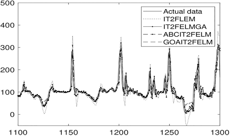
Figure 5: Identification performance of the algorithms for forecasting of electrical power prices at Victoria region

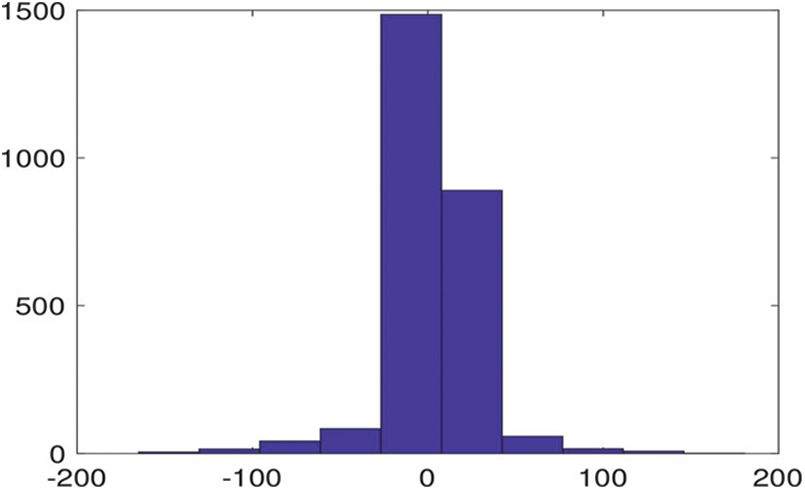
Figure 6: Histogram of error associated with GOAIT2FELM for forecasting of electrical power prices at Victoria region

4.2 Electrical Power Load Demand at Queensland Region

As the second dataset, electrical power load demand at Queensland region is predicted using the proposed approach. The overall number of samples for this case study is 8688 which split into train and test data samples with ratio of 70/30 for train and test data samples. Similar to the previous case, data is treated as a time series whose future 30 minute values depend on the current and three consecutive previous time delayed values of data.

The statistics associated with this dataset are presented in Tab. 1. The minimum value associated with this electricity load demand is 4578.5 and its maximum is 9988.1. The mean value and the standard deviation of this load demand are 6413.3 and 890.7, respectively. Hence similar to the previous case, this dataset is a highly varying dataset.

Tab. 4 presents the comparison result between the proposed algorithm and ABCIT2FELM, GAIT2FELM, and IT2FELM. The proposed algorithm outperforms the other mentioned algorithm (reported in Tab. 4.) except GAIT2FELM both in terms of mean values and standard deviations of RMSE as well as SMAPE. This means that not only the proposed approach acts better than the two other methods but also it is more consistent. Forecast performance of the proposed algorithm vs. ABCIT2FELM, GAIT2FELM and IT2FELM are presented in Fig. 7. Forecasting with good performance can be seen in Fig. 7.

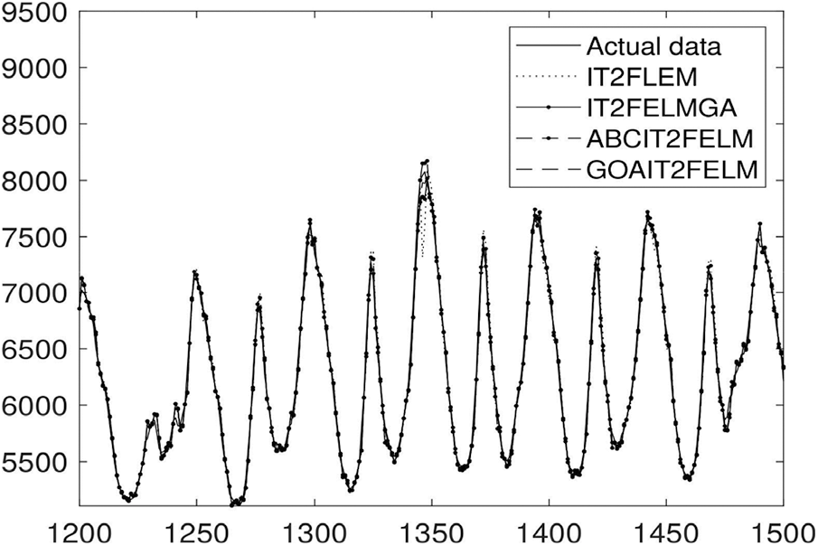
Figure 7: Identification performance of four algorithms for power load demand at Queensland region

Fig. 8 demonstrates the probability distribution function of the error associated with the proposed GOAIT2FELM. As can be seen from the figure that the probability distribution function of error is close to a Gaussian function which is highly desirable.

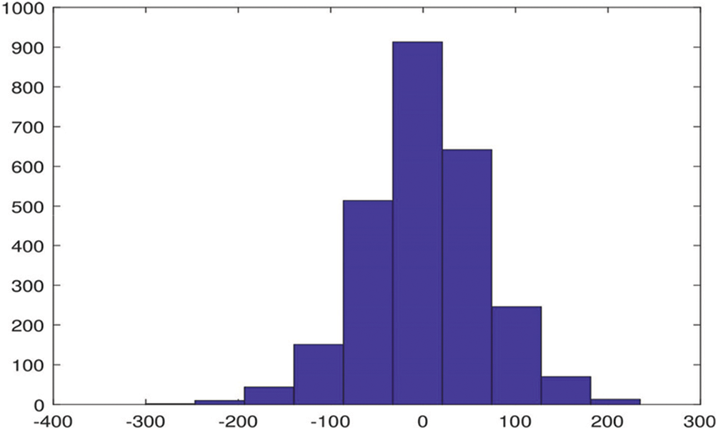
Figure 8: Histogram of error associated with the proposed GOAIT2FELM for power load demand at Queensland region

The evolution of RMSE during the optimization using the proposed GOAIT2FELM vs. other two algorithms of ABCIT2FELM and GAIT2FELM is depicted in Fig. 9. The evolution of the proposed approach is faster that the other two optimization algorithms.

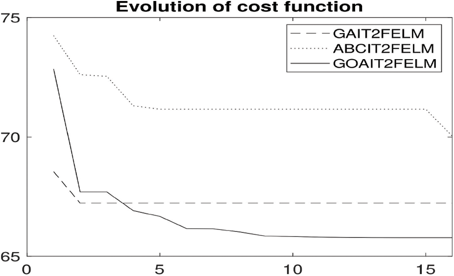
Figure 9: Evolution of RMSE during optimization using the three optimization algorithms

4.3 Electricity Power Price at Queensland Region

As the third dataset, electricity power price at Queensland region is predicted using the proposed approach. Similar to the previous two cases, the total number of samples in this case is equal to 8688 which split between train and test data samples of 70/30. The inputs taken for the predictor are similar to the previous case, i.e., taking the future 30 min values to be dependent upon the current and three consecutive previous time delayed values of data with the sample time of 30 minutes.

The statistics specification of electricity power price in Queensland region are presented in Tab. 1. These statistics show that this dataset is a highly varying dataset with its minimum value equal to −261.3 and its maximum being equal to 1223.3. The mean value and the standard deviation of this electricity price dataset are 80.9 and 34.3, respectively.

Tab. 5 illustrates the comparison result between the proposed algorithm and ABCIT2FELM, GAIT2FELM, and IT2FELM in terms of RMSE and SMAPE. Tab. 5 reports that using GOAIT2FELM, it is possible to forecast data with higher performance in terms of mean values and standard deviations over 10 times of run of programs. It is further noticed during simulation that IT2FELM failed to perform the optimization in one run over 10 times run of programs which resulted in a very large RMSE. Overall Tab. 5 shows that the proposed approach acts better than the three other methods and it is a more consistent algorithm. Hence, it is expected that the proposed approach result in a superior performance than the other two approaches in every single run of program with a high probability. Forecast performance of all algorithms are presented in Fig. 10. It can be seen that the proposed model's prediction is achieved with high performance . Moreover, it can be inferred from Fig. 10 that the results obtained by IT2FELM are the furthest from the electrical power demand at Queensland area. This result is what we expect from this training algorithm as it does not provide any means to estimate the AP parameters.

Probability distribution function associated with the proposed GOAIT2FELM is presented in Fig. 11 which demonstrates the probability distribution function of the error associated with the proposed GOAIT2FELM has the properties of a Gaussian function which basically having a very large value close to its mean value and gradually decreases to a very small value.

The general trend of RMSE during the optimization using the proposed GOAIT2FELM vs. other two algorithms of ABCIT2FELM and GAIT2FELM is depicted in Fig. 12. This shows that the proposed approach is faster that the other two optimization algorithms as well.

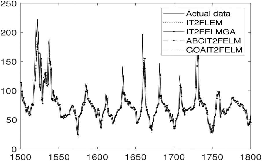
Figure 10: Forecasts for electricity power price for Queensland region using all four algorithms

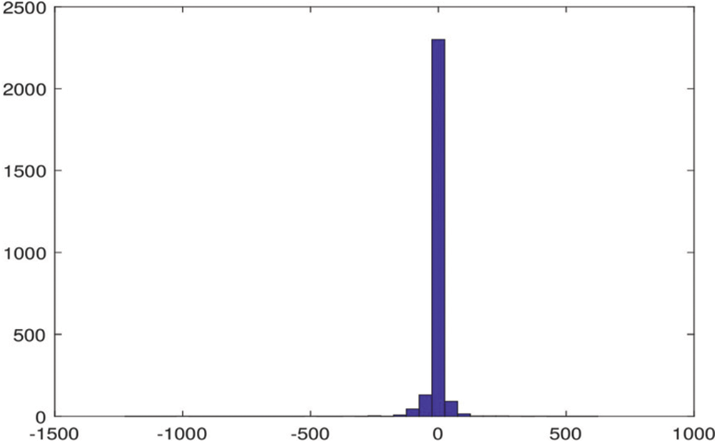
Figure 11: Histogram of error associated with electricity power price for Queensland region using GOAIT2FELM

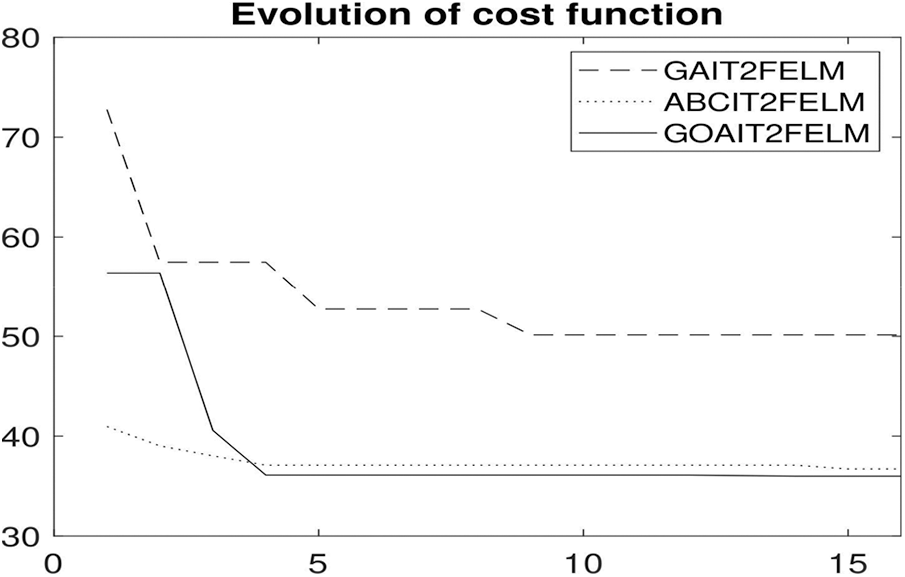
Figure 12: Evolution of RMSE during optimization for electricity power price for Queensland region

5  Conclusions

A hybrid parameter estimation method is proposed for IT2-FLSs which is a modified version of IT2FELM. IT2FELM is a two stage parameter estimation algorithm for the parameters of IT2-FLSs. However, IT2FELM does not include any means to estimate the AP parameters of IT2FELM. In this paper, GOA which is a recent optimization algorithm is used for the AP parameters and IT2FELM is used for the CP parameters. Simulation results demonstrate that using GOA for the AP parameters improves the the overall prediction performance using IT2-FLSs. The proposed hybrid algorithm is called GOAIT2FELM and is compared with ABCIT2FELM, GAIT2FELM and IT2FELM. The proposed algorithm is used for the prediction problem of electricity power price of Victoria region in Australia, electricity load demand for Queensland region and electricity power price of the same region. The simulation results demonstrated the superior performance of the proposed approach over ABCIT2FELM, GAIT2FELM and IT2FELM on these applications in terms of RMSE and SMAPE. Not only the results obtained using the proposed approach are better than that of the three other algorithms, they are more consistence which means that in future trials, it is expected to gain superior performance in a single run of the algorithm. The evolution of the proposed GOAIT2FELM is compared against the two estimation algorithms namely ABCIT2FELM and GAIT2FELM which shows that the speed of the convergence of the proposed algorithm is higher than the two other investigated algorithms namely ABCIT2FELM and GAIT2FELM.

Funding Statement: The publication of this article is funded by the Qatar National Library. The authors would like to acknowledge the library for supporting the publication of this article.

Conflicts of Interest: The authors declare that they have no conflicts of interest to report regarding the present study.

This work is licensed under a Creative Commons Attribution 4.0 International License, which permits unrestricted use, distribution, and reproduction in any medium, provided the original work is properly cited.