Computers, Materials & Continua DOI:10.32604/cmc.2022.021629
Article

A Deep Two-State Gated Recurrent Unit for Particulate Matter (PM2.5) Concentration Forecasting

Muhammad Zulqarnain1, Rozaida Ghazali1,*, Habib Shah2, Lokman Hakim Ismail1, Abdullah Alsheddy3 and Maqsood Mahmud4

1Faculty of Computer Science and Information Technology, Universiti Tun Hussein Onn Malaysia, Batu Pahat, Johor, Malaysia
2College of Computer Science, King Khalid University, Abha, Saudi Arabia
3College of Computer and Information Sciences, Imam Mohammad Ibn Saud Islamic University, Riyadh, Saudi Arabia
4Department of Management Information Systems, College of Business Administration, Imam Abdulrahman Bin Faisal University, 31441, Dammam, Saudi Arabia
*Corresponding Author: Rozaida Ghazali. Email: rozaida@uthm.edu.my
Received: 08 July 2021; Accepted: 23 August 2021

Abstract: Air pollution is a significant problem in modern societies since it has a serious impact on human health and the environment. Particulate Matter (PM2.5) is a type of air pollution that contains of interrupted elements with a diameter less than or equal to 2.5 m. For risk assessment and epidemiological investigations, a better knowledge of the spatiotemporal variation of PM2.5 concentration in a constant space-time area is essential. Conventional spatiotemporal interpolation approaches commonly relying on robust presumption by limiting interpolation algorithms to those with explicit and basic mathematical expression, ignoring a plethora of hidden but crucial manipulating aspects. Many advanced deep learning approaches have been proposed to forecast Particulate Matter (PM2.5). Recurrent neural network (RNN) is one of the popular deep learning architectures which is widely employed in PM2.5 concentration forecasting. In this research, we proposed a Two-State Gated Recurrent Unit (TS-GRU) for monitoring and estimating the PM2.5 concentration forecasting system. The proposed algorithm is capable of considering both spatial and temporal hidden affecting elements spontaneously. We tested our model using data from daily PM2.5 dimensions taken in the contactual southeast area of the United States in 2009. In the studies, three evaluation matrices were utilized to compare the overall performance of each algorithm: Mean Absolute Error (MAE), Root Mean Square Error (RMSE), and Mean Absolute Percentage Error (MAPE). The experimental results revealed that our proposed TS-GRU model outperformed compared to the other deep learning approaches in terms of forecasting performance.

Keywords: Deep learning; PM2.5 forecasting; air pollution; two-state GRU

1  Introduction

Particulate matter (PM) levels have recently become a global issue. Atmospheric aerosols are groupings of solid or liquid particles suspended in the air that arise from a variety of sources and come in different shapes and sizes. Furthermore, the majority of particulate matter is formed in the lowest layer of the atmosphere. Fine particles having aerodynamic dimensions less than 10 and 2.5 m are referred to as PM10 and PM2.5 respectively. Many epidemiological studies have demonstrated that PM is extremely harmful to people, especially at high concentrations [1]. PM2.5 is still a major public health concern [2], and it has been related to a number of health consequences, such as cancer, respiratory, mortality, and cardiovascular illnesses [3]. Environmental exposure analysis has increased significantly due to advances in geospatial technologies, particularly Geographic Information Systems (GIS). An adequate knowledge of PM2.5 in a continuous space-time domain is necessary for a useful evaluation of the quantifiable link between adverse health effects and PM2.5 concentrations. Because air pollution data is frequently obtained at discrete or restricted sample areas, it is frequently essential to estimation air quality intensity at current information locations inside the region of a finite set of existing data points, which referred to interpolated in quantitative simulation. Based on the assumption, the spatial interpolation approaches have been already widely examined over the years that are higher associated with ordinary spatial interpolation approaches, including Inverse Distance Weighting (IDW) [4], trend surface [5] and splines [6].

Most well-known interpolation approaches, such as IDW and Kriging, constrain interpolation methods which are commonly described with clear and simple mathematical expression. In contrast to conventional spatial interpolation, spatiotemporal interpolation requires consideration of an additional time dimension. There are some effective and efficient interpolation techniques for complicated spatiotemporal datasets. Some spatiotemporal approaches [7] integrate time and space individually and decrease the temporal interpolated issue to a series of multivariate statistical snapshots. Few other spatiotemporal approaches [8,9] consider time as a separate dimension in space and integrate both temporal and spatial aspects at the same time. Unfortunately, none of the thesis researches provided adequate methodologies for including time aspects, ensuring that the sequential measurement is handled “equitably” in comparison to the spatial dimension. Samal et al. [10] were referred to this issue as the “time scale issue” and later, over the past decades Fioravanti et al. [11] were revised the scaling ratio is known as “spatiotemporal anisotropy parameter”. To estimate this parameter, just a few basic approaches were proposed. The fundamental reason, there is a dearth of strong theoretical assistance for determining the relationship between time and space dimensions. A black box strategy, including the artificial intelligent algorithm, is a reasonable concept and an auspicious way to predict the spatiotemporal assessment parameter in such scenarios. Furthermore, Badli et al. [12] presented an effective parallel machine learning model to address this challenge in order to regulate the appropriate spatiotemporal anisotropy parameters.

Through a hierarchical learning process, deep neural network approaches have extracted high-level, features from data for learning processing [13]. Artificial intelligence inspired the hierarchical learning mechanism, which resembles the deep layered learning mechanism of the core sensory fields of the human brain's neocortex, which pulls functionalities and abstractions from the core input [14,15]. Since its inception, deep learning has been effectively used in time series prediction [16], object detection [17] natural language processing [18], medical images analysis [19] multi-class skin cancer classification [20], and sentiment analysis [21]. Deep recurrent neural network (DRNN) [22] is one of the most suitable deep learning models for time series prediction and sequence modelling because it often perceives the current input but also a trace of formerly obtained data through use of repeatable process, that permits a directly dispensation of sequential relationship and other hidden probability.

Lately, in 2017, Fan et al. [23] introduced a DRNN-based comprehensive forecast architecture for air pollution level. It's a helpful forecasting approach that can't be employed for common interpolation goals. Recently in 2018, Qi et al. [24] proposed broad and efficient technique to address the fine-grained air quality interpolation, forecasting, and feature analysis in one model. The RNN was used as the major ingredient in their method as well. Previous RNN-based deep learning approaches relied solely on historical data. Furthermore, they considered that the present air pollution intensity is solely driven to the concerned point's by previous information and the present air quality strengths of its environmental situations. This argument is flawed because it ignores the time relation between spatial neighbors.

This research intends to create a unique spatiotemporal interpolation technique for predicting PM2.5 based on Two-State Gated Recurrent Unit, which considers both past and future spatiotemporal relationships between geographical neighbours. Our methodology enables the creation of more precise air pollution estimates on a vast geographic area due to long period of time. Generally, RNN's memory of previously acquired patterns fades with time, resulting in a calculation difficulty known as vanishing gradient [25]. We explored the advanced variant of recurrent neural networks such as Gated Recurrent Unit (GRU) [26] GRU handles this problem by retaining an internal flow of information and establishing routes where the gradient can flow for a long period of time. Specifically, we used the Two-State GRU (TS-GRU) to train our prediction model for air pollution concentrations. In particularly, the two-state principle divides the neurons of a developed TS-GRU into two directions, allowing for simultaneous consideration of both past and future information. We assessed the model performance of our proposed model using ground PM2.5 measurements from the US Environmental Protection Agency (EPA)'s Air Quality System (AQS). In order to examine the impact of concentration influence on the temporal dimension, we also compared our developed approaches to the existing GRU RNN model.

2  Related Works

2.1 Spatial Temporal Interpolation

Despite the fact that PM2.5 concentrations are usually observed in common countries including USA, the number of sensors and their geographic range continue restricted. Mostly In any circumstance, none of these studies provide a strategy for predicting pollution over the next several months or identifying associated factors. With ever-increasing levels of air pollution, it's critical to develop efficient air quality monitoring simulations based on data provided by pollution sensors. These algorithms may help predict the concentration of particles and provide an assessment of air pollution in each location. As a result, air quality assessment and forecasting has become a significant study area. In conjunction to pieces within the ensemble that address the hypothesis of air pollution. Advanced spatiotemporal interpolation technique is critical for gaining a good understanding of the observed air pollutants because it can have a significant influence on the precise assessment of humanoid revelation to PM2.5 and obtain more consistent analysis of the correlation among PM2.5 and disease consequences through time [26]. Assume that in an area A, there are n various monitoring stations {S1, . . . ,Sn}. The analysis for particular situation Si at a certain time stamp t can be defined as a tuple xi,t=(loni,lati,t,vi) where vi is the reported air pollutant concentration is measured, loniandlati defining the longitude and latitude of the station Si, accordingly. As a result, the input dataset can be referred to as n time series, {ts1,…,tsn}. The sequential time series ts1=xi,1,…,xi,T that observed by data at a single station Si. Based on the time series the basic purpose of this research is target to estimateA at any time for the position of v. The local air quality is frequently affected by nearby places in the spatial dimension as air pollutants can disseminate or spread across the atmosphere with the wind [27].

Historical air pollution levels can influence present and future levels in the temporal dimension. For example, the pollution levels of the previous hour will have an impact on the next hours of pollution levels during the observation process. Furthermore, some various cases have included in recent years is that, atmosphere has tended to be similar during the same time of periods. In conclusion, to all influencing factors mentioned above, many other factors including weather, human activities and traffic flow can cause changes in air quality in both geographic and frequency domain, affecting air pollutant concentrations. It is difficult to construct a comprehensive mathematical model to estimate the levels of air quality due to the lack of a available dataset and only three affecting parameters, namely longitude, latitude, and time have been used in the recent studies. Although GRU is one of the most effective approaches, it has been applied for the prediction of various types of particulate matter (PM) levels.

2.2 Gated Recurrent Unit (GRU)

The GRU is a more advanced and simplified version of the recurrent neural network such as LSTM, which was first proposed on statistical machine translation by [28]. GRU is based on the LSTM, which uses an update gate zt and a reset gate rt to handle information flow inside the unit without the use of separate memory. As a result, GRU can capture the mapping relationship between time-series data [29,30], while also offering appealing benefits such as reduced complexity and a faster computational procedure. Fig. 1 demonstrate the GRU computational structure, which shows the connection among the update and reset gates. Furthermore, GRU uses internal memory to retain the filter information and combines the input and forget gates into a single update gate with previous state ht−1 and the candidate computation illustrated by h~t. The update gate, reset gate, and candidate state are the three major components of GRU, and their equations summaries as follows:

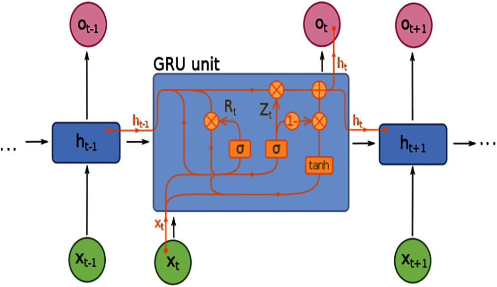
Figure 1: GRU Architecture

zt=φ(Vxzxt+Uhzht−1+Bz)(1)

rt=φ(Vxrxt+Uhrht−1+Br)(2)

h~t=tanh(Vxh~xt+Uhh~(rt∗ht−1)+Bh~)(3)

ht=(1−zt)∗ht−1+zt∗h~t)(4)

where Vxz, Vxr and Vxh~ present to the weights vector between the input layer and update gate, reset gate and candidate vector while weight matrix Uhz, Uhr and Uhh~ referring the recurrent connection respectively. φis the nonlinear activation function of update and reset gates, * conducts multiplication operation between the component and Bz, Br and Bh~ are the associated biases.

3  The Proposed Model: Two-State GRU Mechanism

GRU is the latest kind of traditional RNN which particularly has to be used for sequential modeling. However, a recurrent layer required the input vector ht ∈ Rn at each timestep t, and hidden state ht by implementing the recurrent procedure:

ht=f(Wxt+Uht−1+b)(5)

where W∈Rm∗n,b∈Rm∗m,b∈Rm weights matrix, and element-wise nonlinearity is represented by ƒ. Training the long-term dependencies with RNN is very complicated due to the problem of vanishing gradient and exploding [31]. By applying the gating architecture, GRU can maintain memory substantially better than traditional RNN [32]. However, based on the existing literature, we explored that when GRU analyze a word it only includes the forward semantic information, so it is impossible for GRU to learns the backward contexts. As the results, we also observed that in any language approach, which process of sentence is not affected only through forward information but also in the backward context. Therefore, in this study, we proposed Two-State GRU (TS-GRU) to solve the aforementioned issue. The proposed TS-GRU model consists of two processes, one for positive pass known as “forward pass”, and other for negative pass known as “backward pass” presented in Fig. 2. The two-state GRU can efficiently learn the context through both directions.

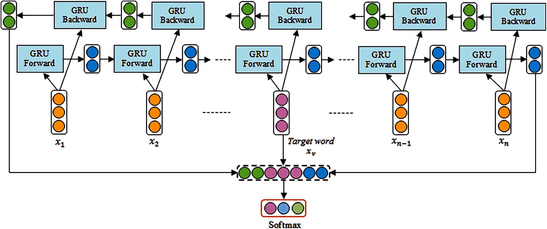
Figure 2: The proposed Two-State GRU architecture for sentiment analysis

TS-GRU is inspired by the bidirectional recurrent neural networks (BRNNs) in [33]. It consists of two separate recurrent nets in the terms of forward passes (left to right (for future information)) and backward passes (right to left (for past information)) in the training process and finally both of them are merged to produce output layer. The formulas for update gate zt, reset gate rt, candidate state h~t, and final output activation state ht of the forward and backward GRU are shown as a follows:

Forward pass:

zt→=σ(Wzx→xt)+Uzh→ht−1→+bz→)(6)

rt→=σ(Wrx→xt)+Urh→ht−1→+br→)(7)

h^t→=tanh(Wh^→xt)+rt→∗Uh^→ht−1→+bh^→)(8)

ht→=(1−zt→)∗ht−1→+zt∗h^t→)(9)

Additionally, we implemented backward pass in the proposed approach to explore more valuable information.

Backward Pass:

zt←=σ(Wzx←xt)+Uzh←ht−1←+bz←)(10)

rt←=σ(Wrx←xt)+Urh←ht−1←+br←)(11)

ht←=tanh⁡(Wh←xt)+rt←∗Uh←ht−1←+bh←)(12)

ht←=(1−zt←)∗ht−1←+zt∗h^t←)(13)

The activation of a word at time t: ht=[ht→,ht←] = for an arbitrary sequence (x1,x2,…,xn) containing n words, at time t each word illustrated as a dimensional vector. The forward GRU computes ht→ which takes left-to-right contexts of the sentence whereas the reverse GRU consider right-to-left contexts ht← for attention. Then forward and backward context descriptions are then combined into a single context. In common, Backpropagation Through Time (BPTT) is a gradient constracted based methodology and a veriation of the conventional backpropagation method that can be used to train the DRNN (Chauvin and Rumelhart 1995) [34]. BPTT starts with development of a unfolding RNN in time so that each timestep has one input timestep, one copy of the network, and one output.

The system flow diagram of the proposed TS-GRU is presented in Fig. 3. During training to avoid being excessively fractional to a particular dimension, the original dataset is first normalized, that is, the data points of all dimensions are constrained to a range of 0 to 1. Furthermore, the regularized data is divided into two sections: training data and testing data. Only the training data is used throughout the training to maintain the impartiality of performance evaluation. When training data is fed into the TS-GRU, a loss value is created, and the enhancement adjusts the parameters of TS-GRU using the backpropagation method. The forecasting performance of TS-GRU will become more precise with the increase of training iterations. The testing data is entered into the TS-GRU when the learning is finished, and evaluate the performance of the TS-GRU the testing results and real results were compared. Overfitting can happen when there is not enough training data or when there is too much training.

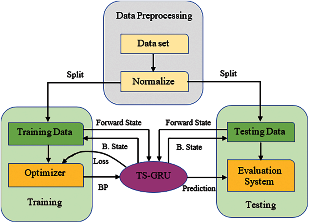
Figure 3: The system flow diagram of the proposed TS-GRU

However, overfitting can be avoided using several methods including, regularization [35], data augmentation [36], dropout [37], and dropconnect [38]. Regularization can be divided into two types: L1 regularization and L2 regularization, both of which are commonly employed in deep learning. To avoid overfitting, both of these strategies minimize the weight value of the neural network as much as possible. The goal of data augmentation is to enhance the dimension of the dataset as much as conceivable, for example, by adding random bias or noise, in order to diversity the training data and improve training results. Dropout and dropconnect are similar in that the former pauses the neuro's operation at random, while the latter eliminates the connection at discrete points. The early stopping technique is implemented in this paper [39].

4  Experimental Design

In this section, we briefly explained the experimental settings, measure of performance and empirical results of the developed two-state GRU approach.

4.1 Data Set Description

We investigated the daily PM2.5 data set in Florida in 2009 to illustrate the performance and efficiency of our developed approach. This data was accessed by the United States Environmental Protection Agency's Air Quality System (AQS) controlling process and can be accessible via EPA's website. In this dataset, a tuple entry (t,lon,lat,v), is determined by each dataset where lon and lat are referring to the length and parallel coordinates of the controlling station, t=(year,month,day) representing the date when a PM2.5 dimension is reserved, and v is the calculated PM2.5 value. Tab. 1 shows the separate entity from one controlling station. The extracted features from dataset defined the collection of n time series {ts1,…,tsn} from n controlling positions. Each time series tsi=xi,1,…,xi,T is an sequential observation of data at a one station Si, and xi,t=(t,lon,lat,v) represents one assessment from each station Si at a certain time step t. We can notice from the sample data that the range of raw information fluctuates greatly. Suppose, the [1,12] is the range features of the month, whereas the limit of PM2.5 values is (0, 210]. As a result, we measure the informative features so that all values fall between 0 and 1. Moreover, Ioffe et al. [40] also shown that when features are scaled, gradient descent converges substantially faster.

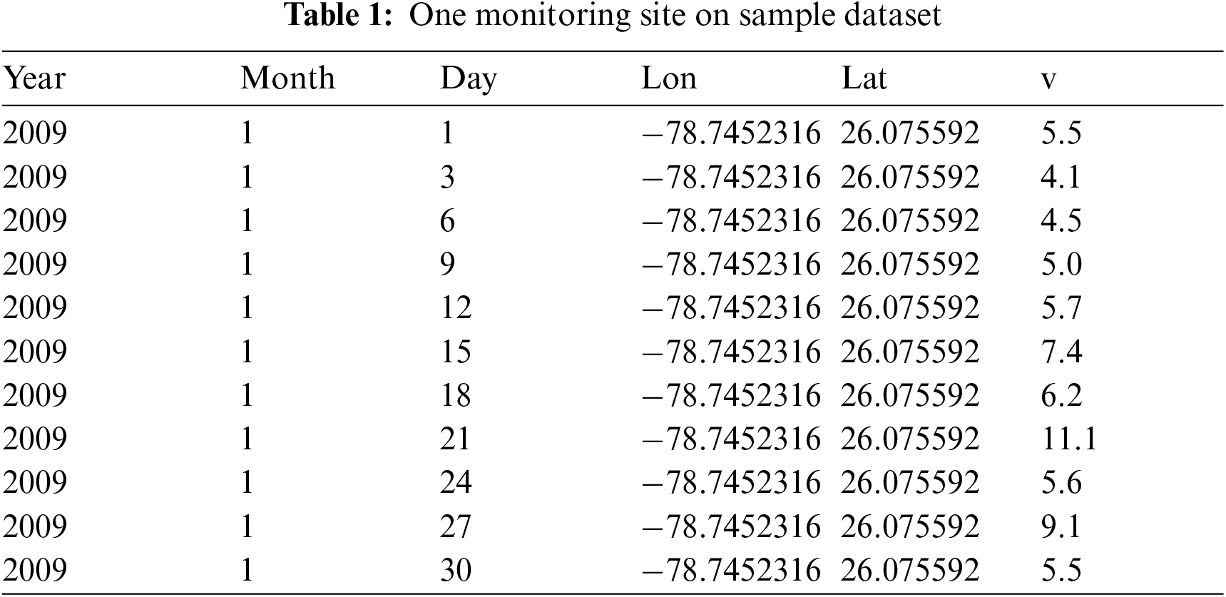
The original dataset consists incorrect entries, indicating that no measurements were taken at a distinct location and on a specific day. There were 6,698 everyday proportions at 30 controlling locations on all 365 days of 2009 after eliminating all the incorrect entries.

4.2 Implementation Detail and Parameter Settings

In the temporal interpolation, we assume that reginal pollution levels are influenced not just in nearby fields, but similarly associated by factual and prospective information from surrounding places [41]. Our proposed framework uses the TS-GRU (illustrated in Fig. 2) to collect the both geographical and temporal relationships. In the proposed framework two directions GRU layers and conventional dense layers are stacked in the network. Furthermore, the random uniform approach is used to set the parameters of each layer randomly and equally, and the sigmoid nonlinear process is utilized to imitate non-linearity in each layer. We used MAPE as our loss function because of its scale independence and interpretability. Finally, we used Adam algorithm [42] to train and optimized the entire neural network, which is a numerically effective technique for rapid stochastic optimization. Kingma and Ba showed that, Adam algorithm is suitable for issues with enormous amounts of data and is also suitable for non-stationary goals [42]. All the simulations of this research were implemented on Intel core-i7-3770 CPU @ 3.40 GHz, DDR3 and 8 GB of RAM with Window 10 operating system. We used Python 3.7 compiler and a high-level NNs API-Keras as the development environment, with required libraries TensorFlow 1.14 and Keras 2.3.

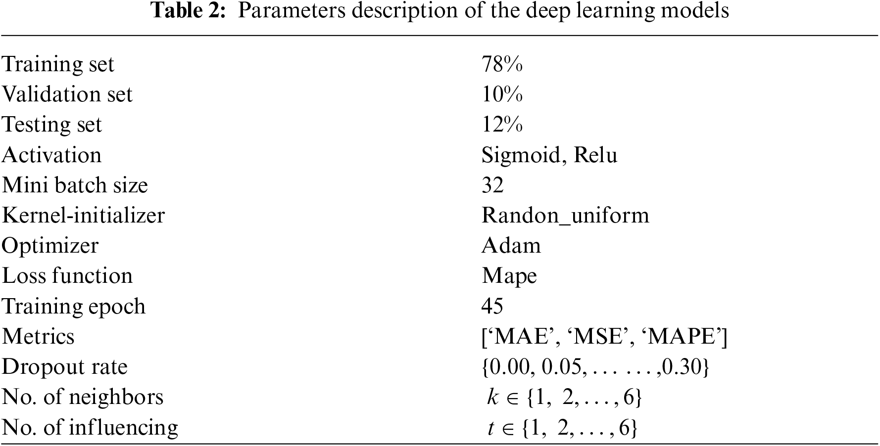
It is usual to run into the overfitting issue, when training neural network algorithm (see Tab. 2. for the details), which indicates the performance of both training and testing set. However, the training set is substantially superior than testing set. To solve the overfitting issue and enhance the robustness of our approach, we used the k-fold cross validation [43] and dropout technique [37]. We divide the dataset into k equivalent-size subgroups for k-fold cross validation, then choose one subset as the testing set and train on the subsisting k–1 subset iteratively. In this study, we used the generally utilized 10-fold cross validation method. As a result, we randomly partition our dataset into 78% training set, 10% validation set and 12% testing test, and then train our network on the training set using the 10-fold cross validation technique.

When training a neural network, the dropout technique works by sampling a “thinned” model. To optimize the model, we arbitrarily selected a portion of nodes in hidden layer and temporarily deleted them from the network, as well as all input and output connectivity at each iteration. As a side effect, the dropout technique also improves the training efficiency by requiring fewer computations. We also explored that the actual air quality is strongly linked to air quality levels in the past and future days.

4.3 Evaluation Methods

In this paper, we employed three assessment measures to access the performance of the developed model. When comparing predictions to actual values, these metrics were calculated: mean absolute error (MAE), root-mean-square error (RMSE), and mean absolute percentage error (MAPE). Smaller values indicate better performances. The Large error are given relatively high weights by the RMSE. These equations are follows:

MAE=1N∑i=1N⁡|Oi−Pi|(14)

MAPE=1N∑i=1N⁡|Oi−Pi|Oi(15)

RMSE=1N∑i=1N⁡(Oi−Pi)2(16)

where Oi represents the observed air quality, while predicted air quality denoted by Pi, and the number of assessment samples showed by N. The absolute error is calculated using the previous two indices, whereas the relative error is calculated using the third. In other words, the extreme consequence and error scope of the projected values are expressed by RMSE and MAE, while the specificity of the average projected value is represented by MAPE [44].

5  Results and Discussion

In this section, three experiments were conducted to investigate the spatiotemporal relationships and to illustrate the efficacy of our proposed methodology.

Experiment 1: network architecture to insert our spatiotemporal dataset, we initially investigated appropriate deep learning architecture. The purpose of our first experiment is determined to stability the efficacy of our spatial and temporal interpolation technique by selecting the dropout rate, epoch numbers, and batch size. We consider that both the variables of closest neighbors and the quantity of the influencing days are 1, i.e., k=1,t=1. In this experiment, the training set is separated through a number of constant dimension batches during the neural network training, in which each batch being transformed in order to during one learning session. As a result, we notice that the gradient and frequency of weights updates by batch size. Smaller batch sizes are usually encountered in less training epochs, whereas higher batch sizes provide additional similarity and thus superior calculation competence, as the separate learning instances within a single batch might be procedure in similar [45]. In this study, we experimented with numerous batch sizes because our training data set is rather tiny, with only about 7,000 entrances. we experimented with several batch sizes {4, 8, 16, 32, 64, 128, 256}. Tab. 3 illustrates the results. Finally, we selected 32 as our batch size to attain a proportion among the computational efficacy and competence. An epoch is a single pass over the complete training set batch by batch. The drawbacks of neural networks include the possibility of overfitting and a high computational cost.

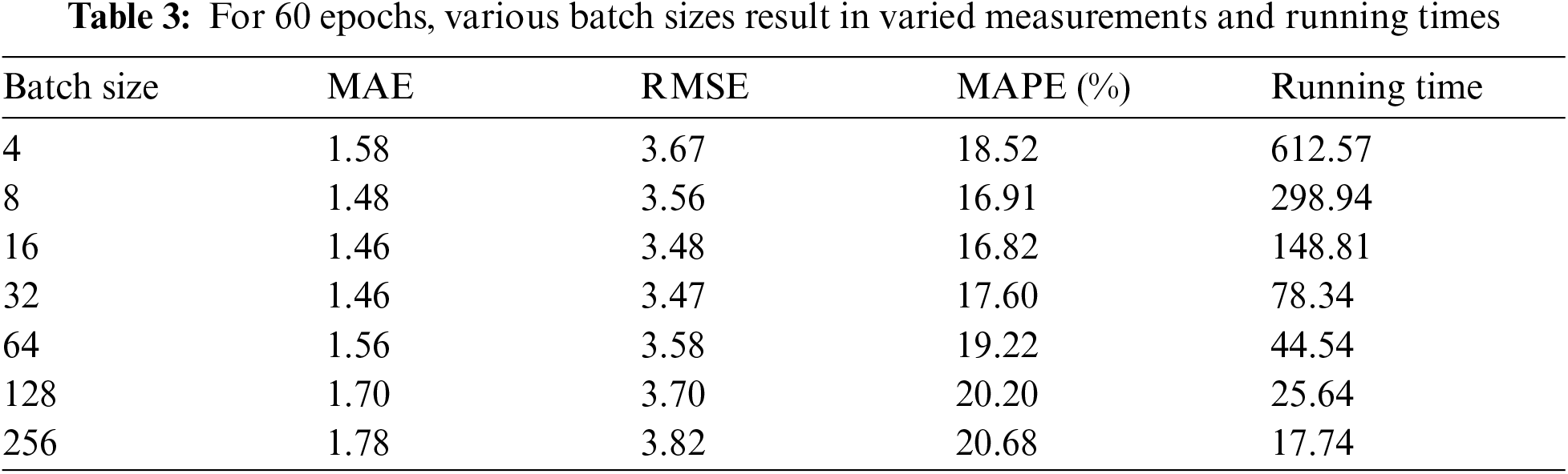
We trained our model over 60 epochs when the batch size was 32, and the temporal training and validation losses were reported in Fig. 4. During the training process, we noticed that both kinds of losses generally remain constant when the epoch number is greater than 45. Therefore, for our subsequent experiments, we set the epoch number up to 45. As we discussed in the previous section, the dropout technique is employed to enhance the performance of our developed approach by neglecting a smaller faction of interconnections at randomly. We have attempted eight various dropout rates to determine the dropout rate: {0.00, 0.05, 0.10, 0.15, 0.20, 0.25, 0.30, 0.35}. Tab. 4 contains the statistical data, and Fig. 5. Depicts a performance of MAPE in the term of visualizations representation. In this case, we noticed that the values of MAPE increases as the dropout rate increases, as shown in Fig. 5. Which indicates a weak model for a higher dropout rate.

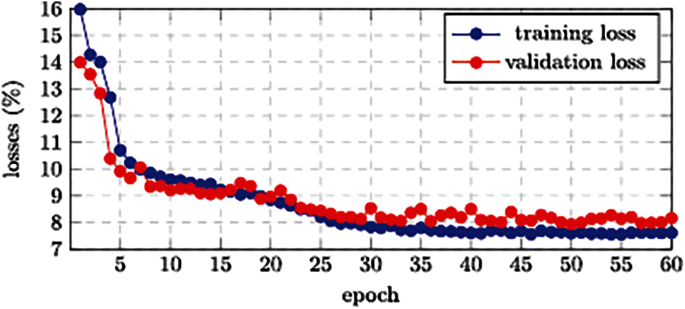
Figure 4: The training and validation losses

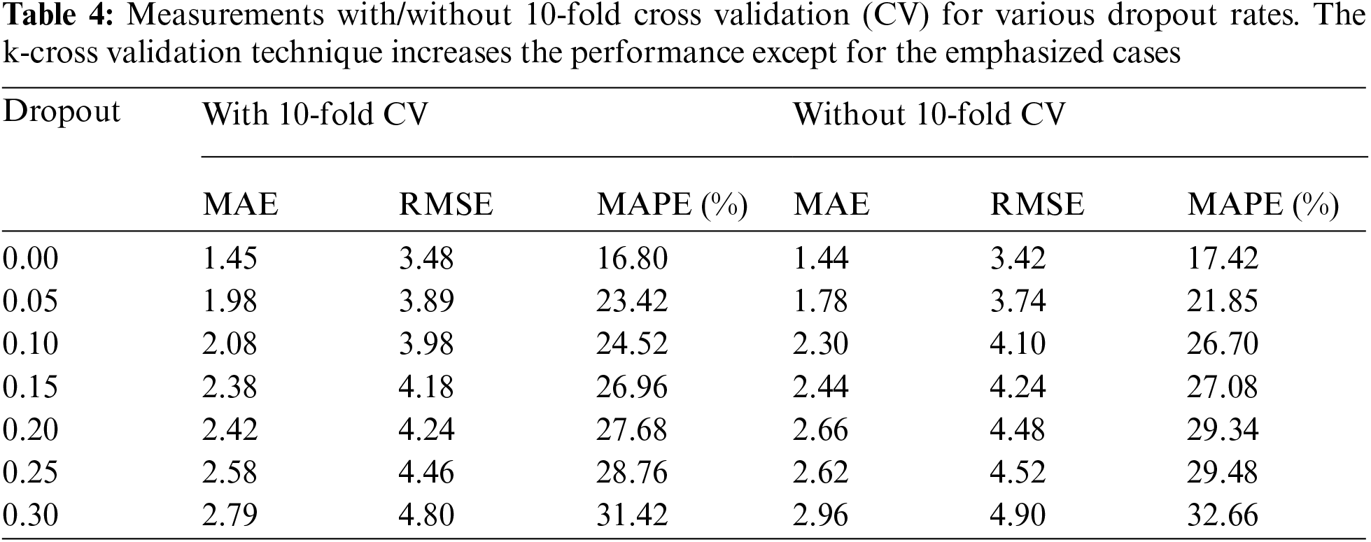
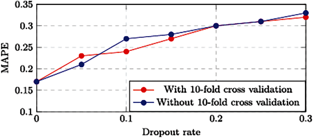
Figure 5: MAPE for various dropout rate

For improving the performance of our developed approach, we adopted another approach, 10-fold cross-validation, during the training procedure. The previous experiment was replicated without the 10-fold cross validation approach, as well as the findings are summarized in Tab. 4. The 10-fold cross validation certainly enhance the robustness of our developed approach in the vast majority of scenarios.

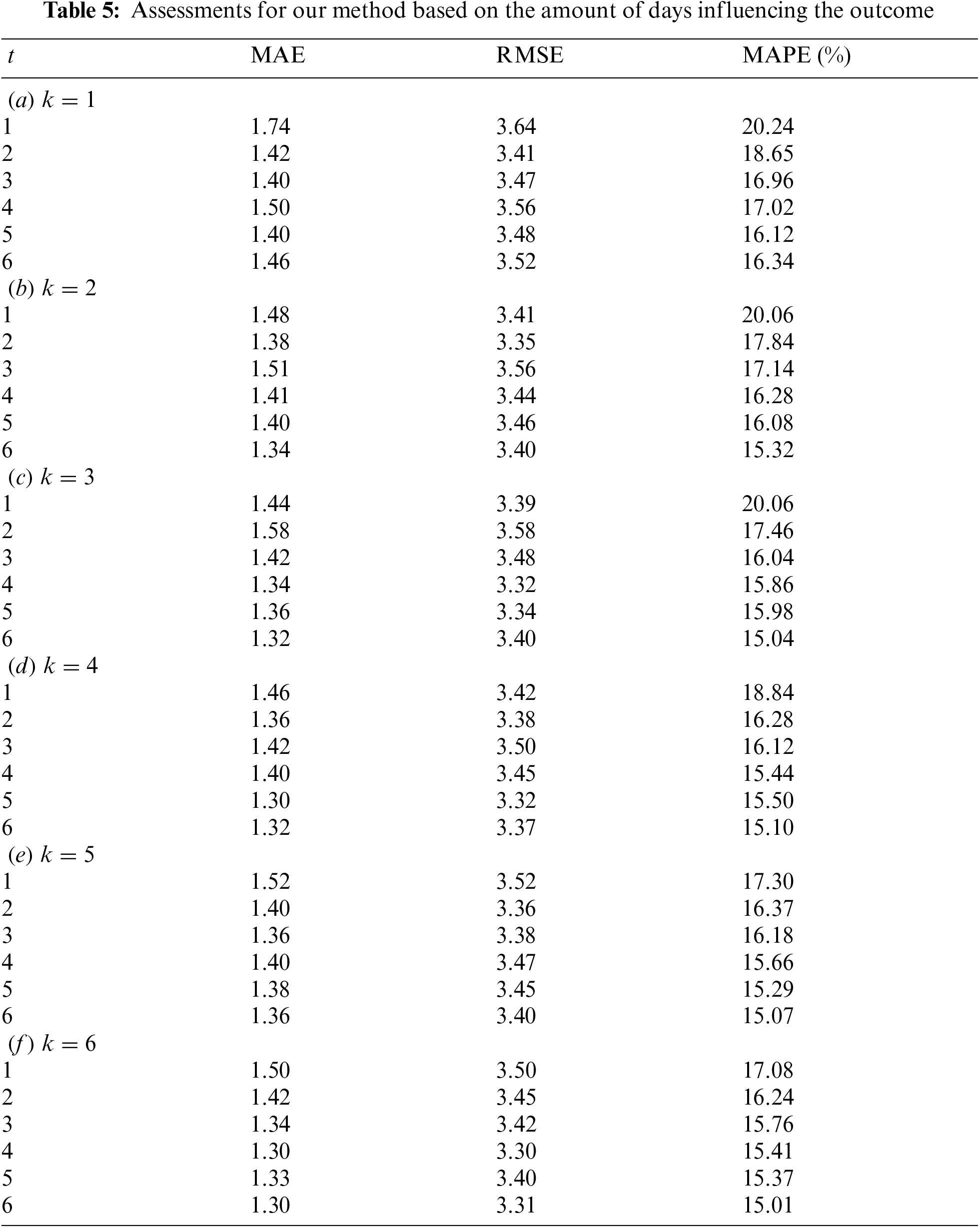
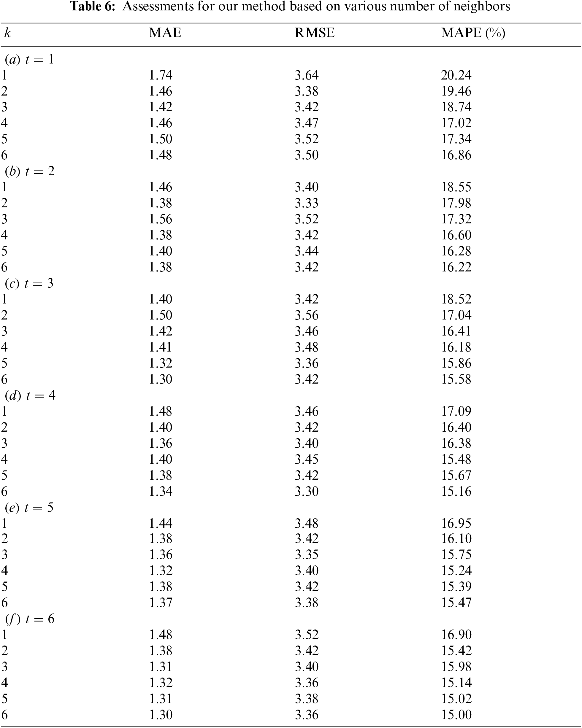
Experiment 2: number of influencing neighbors and days We examined various k and t at the interested point to investigate how environmental and sequential neighbours affect air quality. We set k∈{1,2,3,4,5,6} and t∈{1,2,3,4,5,6} in a more specific way. Tabs. 5 and 6 reported the statistical measurements were collected by experiment. In this experiment, we noticed that during the training process the network takes into the account additional geographical neighbours of the interested site and the MAPE tends to reduces. On the other hand, when the network considers further previous and future days, these reducing features probably applies.

Experiment 3: comparison with GRU-base RNN In our final experiment, we compared the developed TS-GRU model with the existing deep GRU discover if the present condition of the air quality is associated with the future outcomes. In this experimental procedure, we build a GRU-based deep RNN, that is comparable to the network in Fig. 2 besides that the Two-State GRU layers are adjusted as the standard GRU architecture. In the GRU, we suppose that the existing level of air pollution is unaffected by descriptive statistics. In other words, the existing GRU is a spatiotemporal prediction network. As a experimental results, the left subfigure of Fig. 6 depicts a three-dimensional mesh representation of the MAPE values. On the right side, a three-dimensional mesh representation for the TS-GRU is illustrated for comparison. When we compared to the present GRU, the MAPE values reduces as k or t increases, which is a comparable observation of GRU. However, the intensity is much smaller for the GRU. Another interesting observation has been made. The GRU attains superior results than the TS-GRU when t is small (t ≤ 3) no matter what k is. In contract, if t is substantial adequate, i.e., k>3, the TS-GRU got remarkable performance than traditional GRU for all k values. More particularly, historical levels of air pollution have a greater impact on future levels of air pollution.

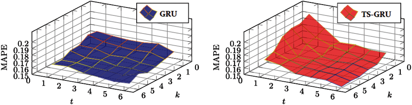
Figure 6: MAPE for traditional GRU and the proposed TS-GRU models

Despite the fact that the TS-GRU model analyses based on informative contents from the future, the near future data brings extra unpredictability or uncertainty into the system, causing the TS-GRU to perform poorly when t is small. The existing GRU approach picks up noise from the past information, whereas the TS-GRU model can calibrate these noises through future information. As a result, the TS-GRU illustrates excellent performance as compared to existing GRU when t is large enough.

Fig. 7 presents the comparison analysis of four experimental approaches. The real data is shown by the solid blue line. Usually, the LSTM and GRU models showed the poor match to the actual data, whereas another hybrid model was consistent. The hybrid approach mostly performed superior than the single approaches. In order to forecasting PM2.5 levels, both the GRU and LSTM approaches were ineffective in forecasting the future higher and lower levels. The hybrid approach predicts the extreme events and commonly outperforms the single approaches. The proposed TS-GRU approach remarkable predicted PM2.5 concentration levels, as compared to hybrid CNN–GRU model over 3 days in the term of future hours. The proposed TS-GRU model outperformed as compared to existing approaches and might be used to predict high PM concentrations in the future.

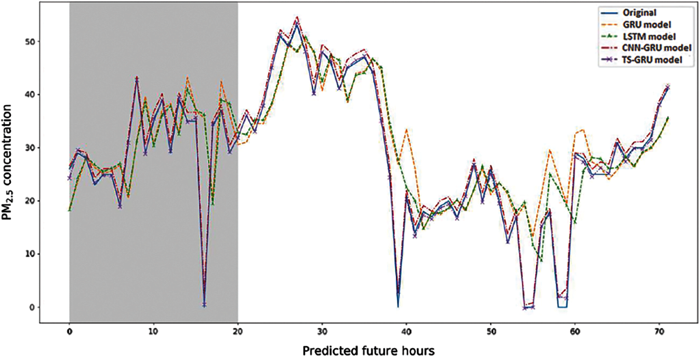
Figure 7: Predicted 3-day PM2.5 concentration; all approaches

6  Conclusion

In this study, we proposed a novel spatiotemporal technique for interpolating PM2.5 concentrations based on Two-State gated recurrent unit. This technique is based on recently proposed deep learning techniques and considers both spatial and temporal aspects simultaneously. In order to remember facts from the past as well as the future, we used the Two-State GRU to split the neurons of an existing GRU into two directions. The particulate matter (PM2.5) predictions are done using deep learning approaches based on the statistical computations of parameters including; MAE, RMSE and MAPE. The results illustrate that our proposed model is perform superior than the existing approaches and also present the actual values and predicted values are very near to each other. To the best of our observation, it is the first time that the Two-State GRU has been used in the spatiotemporal interpolation of air pollutants concentrations. Our future research will focus on this technique for further investigation on ground PM2.5 measurements as well as auxiliary data such as satellite-derived aerosol optical depth (AOD), land use, roads, elevation, and weather circumstances. We will also further investigate the robustness of this strategy for prediction of other pollutant concentrations including ozone (O3) and nitrogen dioxide (NO2) and increase our research field to cover a larger geographical domain. In the future research, we will also explore how to speed up the developed model through using cluster computing frameworks.

Acknowledgement: The authors thank to King Khalid University of Saudi Arabia for supporting this research under the grant number R.G.P. 1/365/42.

Funding Statement: This research work supported by Khalid University of Saudi Arabia under the grant number R.G.P. 1/365/42.

Conflicts of Interest: The authors declare that they have no conflicts of interest to report regarding the present study.

References

 1.  F. Lu, D. Xu, Y. Cheng, S. Dong, C. Guo et al., “Systematic review and meta-analysis of the adverse health effects of ambient PM2.5 and PM10 pollution in the Chinese population,” Environmental Research, vol. 136, pp. 196–204, 2015. [Google Scholar]

 2.  B. M. Balter and M. V. Faminskaya, “Irregularly emitting air pollution sources: Acute health risk assessment using AERMOD and the monte carlo approach to emission rate,” Air Quality Atmosphere & Health, vol. 10, no. 4, pp. 401–409, 2017. [Google Scholar]

 3.  E. N. Schachter, E. Moshier, R. Habre, A. Rohr, J. Godbold et al., “Outdoor air pollution and health effects in urban children with moderate to severe asthma,” Air Quality Atmosphere & Health, vol. 9, no. 3, pp. 251–263, 2016. [Google Scholar]

 4.  D. Shepard, “Two-dimensional interpolation function for irregularly-spaced data,” in Proc. of the 1968 23rd ACM National Conf., Cambridge, Massachusetts, pp. 517–524, 1968. [Google Scholar]

 5.  T. Vogl, K. Sripathy, A. Sharma, P. Reddy, J. Sullivan et al., “Radiation tolerance of two-dimensional material-based devices for space applications,” Nature Communications, vol. 10, no. 1, pp. 1–10, 2019. [Google Scholar]

 6.  C. de Boor, “A practical guide to splines,” Mathematical Computing, vol. 34, no. 149, pp. 325, 1980. [Google Scholar]

 7.  A. Appice, A. Ciampi, D. Malerba and P. Guccione, “Using trend clusters for spatiotemporal interpolation of missing data in a sensor network,” Journal of Spatial Information Science, vol. 6, no. 12, pp. 119–153, 2013. [Google Scholar]

 8.  E. Pebesma, “Spacetime: Spatio-temporal data in R,” Journal of Statistical Software, vol. 51, no. 7, pp. 1–30, 2012. [Google Scholar]

 9.  L. Li, T. Losser, C. Yorke and R. Piltner, “Fast inverse distance weighting-based spatiotemporal interpolation: A web-based application of interpolating daily fine particulate matter PM2:5 in the contiguous U.S. using parallel programming and k-d tree,” International Journal of Environmental Research and Public Health, vol. 11, no. 9, pp. 9101–9141, 2014. [Google Scholar]

10. K. Samal, K. S. Babu and S. K. Das, “Spatio-temporal prediction of air quality using distance-based interpolation and deep learning techniques,” EAI Endorsed Transactions on Smart Cities, vol. 5, no. 14, pp. e4, 2021. [Google Scholar]

11. G. Fioravanti, S. Martino, M. Camelett, and G. Cattani, “Spatio-temporal modelling of PM10 daily concentrations in Italy using the SPDE approach,” Atmospheric Environment, vol. 248, pp. 118192, 2021. [Google Scholar]

12. C. Badii, S. Bilotta, D. Cenni, A. Difino, P. Nesi et al., “High density real-time air quality derived services from IoT networks,” Sensors (Switzerland), vol. 20, no. 18, pp. 1–26, 2020. [Google Scholar]

13. M. M. Najafabadi, F. Villanustre, T. M. Khoshgoftaar, N. Seliya, R. Wald et al., “Deep learning applications and challenges in big data analytics,” Journal of Big Data, vol. 2, no. 1, pp. 1–21, 2015. [Google Scholar]

14. H. Patel, A. Thakkar, M. Pandya and K. Makwana, “Neural network with deep learning architectures,” Journal of Information and Optimization Sciences, vol. 39, no. 1, pp. 31–38, 2018. [Google Scholar]

15. S. Pouyanfar, S. Sadiq, Y. Yan, H. Tian, Y. Tao et al., “A survey on deep learning: Algorithms, techniques, and applications,” ACM Computing Surveys (CSUR), vol. 51, no. 5, pp. 23–51, 2018. [Google Scholar]

16. M. Zulqarnain, R. Ghazali, M. G. Ghouse, Y. M. M. Hassim and I. Javid, “Predicting financial prices of stock market using recurrent convolutional neural networks,” International Journal of Intelligent Systems and Applications, vol. 12, no. 6, pp. 21–32, 2020. [Google Scholar]

17. K. Kang, H. Li, J. Yan, X. Zeng, B. Yang et al., “T-cnn: Tubelets with convolutional neural networks for object detection from videos,” IEEE Transactions on Circuits and Systems for Video Technology, vol. 28, no. 10, pp. 2896–2907, 2017. [Google Scholar]

18. T. Young, D. Hazarika, S. Poria and E. Cambria, “Recent trends in deep learning based natural language processing,” IEEE Computational IntelligenCe Magazine, vol. 13, no. 3, pp. 55–75, 2018. [Google Scholar]

19. G. Litjens, T. Kooi, B. E. Bejnordi, A. A. A. Setio, F. Ciompi et al., “A survey on deep learning in medical image analysis,” Medical Image Analysis, vol. 42, no. 8, pp. 60–88, 2017. [Google Scholar]

20. S. S. Chaturvedi, J. V. Tembhurne and T. Diwan, “A multi-class skin cancer classification using deep convolutional neural networks,” Multimedia Tools and Applications, vol. 79, no. 39, pp. 28477–28498, 2020. [Google Scholar]

21. M. Zulqarnain, S. A. Ishak, R. Ghazali, N. M. Nawi and M. Aamir, “An improved deep learning approach based on variant two-state gated recurrent unit and word embeddings for sentiment classification,” International Journal of Advanced Computer Science and Applications, vol. 11, no. 1, pp. 594–603, 2020. [Google Scholar]

22. Y. Gao and D. Glowacka, “Deep gate recurrent neural network,” in 8th Asian Conf. on Machine Learning, PMLR, The University of Waikato, Hamilton, New Zealand, pp. 350–365, 2016. [Online]. Available: http://arxiv.org/abs/1604.02910. [Google Scholar]

23. J. Fan, Q. Li, J. Hou, X. Feng, H. Karimian et al., “A spatiotemporal prediction framework for air pollution based on deep RNN,” ISPRS Annals of the Photogrammetry, Remote Sensing and Spatial Information Sciences, vol. 4, no. 15, pp. 15–22, 2017. [Google Scholar]

24. Z. Qi, T. Wang, G. Song, W. Hu, X. Li et al., “Deep air learning: Interpolation, prediction, and feature analysis of fine-grained air quality,” IEEE Transactions on Knowledge and Data Engineering, vol. 30, no. 12, pp. 2285–2297, 2018. [Google Scholar]

25. C. W. Ruiz, J. Perapoch, F. Castillo, S. Salcedo and E. Gratacós, “Learning long-term dependencies with gradient descent is difficult,” IEEE Transactions on Neural Networks, vol. 66, no. 2, pp. 53–61, 1994. [Google Scholar]

26. Y. Bezyk, I. Sówka, M. Górka and J. Blachowski, “GIS-Based approach to spatio-temporal interpolation of atmospheric CO2 concentrations in limited monitoring dataset,” Atmosphere, vol. 12, no. 3, pp. 384, 2021. [Google Scholar]

27. W. Mao, W. Wang, L. Jiao, S. Zhao and A. Liu, “Modeling air quality prediction using a deep learning approach: Method optimization and evaluation,” Sustainable Cities and Society, vol. 65, pp. 102567, 2021. [Google Scholar]

28. K. Cho, V. B. Merrienbore, C. Gulcehre, D. Bahdanau, F. Bougaress et al., “Learning phrase representations using RNN encoder-decoder for statistical machine translation,” arXiv preprint arXiv, no. 9, pp. 1–15, 2014. [Google Scholar]

29. R. Ghazali, N. A. Husaini, L. H. Ismail, T. Herawan and Y. M. M. Hassim, “The performance of a recurrent HONN for temperature time series prediction,” in 2014 Int. Joint Conf. on Neural Networks (IJCNNno. July, Beijing, China, pp. 518–524, 2014. [Google Scholar]

30. G. Shen, Q. Tan, H. Zhang, P. Zeng and J. Xu, “Deep learning with gated recurrent unit networks for financial sequence predictions sequence predictions,” Procedia Computer Science, vol. 131, pp. 895–903, 2018. [Google Scholar]

31. A. Hassan and A. Mahmood, “Efficient deep learning model for text classification based on recurrent and convolutional layers,” in 2017 16th IEEE Int. Conf. on Machine Learning and Applications (ICMLAno. December, pp. 1108–1113, 2017. [Google Scholar]

32. M. Zulqarnain, R. Ghazali, Y. M. M. Hassim and M. Aamir, “An enhanced gated recurrent unit with auto-encoder for solving text classification problems,” Arabian Journal for Science and Engineering, vol. 46, pp. 1–15, 2021. [Google Scholar]

33. F. Grégoire and P. Langlais, “Extracting parallel sentences with bidirectional recurrent neural networks to improve machine translation,” in Proc. of the 27th Int. Conf. on Computational Linguistics, Santa Fe, New Mexico, USA, pp. 1442–1453, 2018. [Google Scholar]

34. Y. Chauvin, D. E. Rumelhart, R. Durbin and R. Golden, “Backpropagation: The basic theory,” Backpropagation: Theory, Architecture and Applications, no. 14, pp. 1–34, 1995. [Google Scholar]

35. D. Arpit, Y. Zhou, H. Q. Ngo and V. Govindaraju, “Why regularized auto-encoders learn sparse representation,” in 33rd Int. Conf. Machine Learning ICML 2016, New York, NY, USA, vol. 1, pp. 211–223, 2016. [Google Scholar]

36. J. Wei and K. Zou, “EDA: Easy data augmentation techniques for boosting performance on text classification tasks,” arXiv preprint arXiv:1901.11196, 2019. [Google Scholar]

37. G. Hinton, “Dropout: A simple way to prevent neural networks from overfitting,” Journal of Machine Learning Research, vol. 15, no. 1, pp. 1929–1958, 2014. [Google Scholar]

38. C. Y. Lee, P. Gallagher and Z. Tu, “Regularization of neural networks using dropConnect,” IEEE Transaction Pattern Analysus Machine Intelligent, vol. 40, no. 4, pp. 863–875, 2018. [Google Scholar]

39. C. J. Huang and P. H. Kuo, “A deep cnn-lstm model for particulate matter (PM2.5) forecasting in smart cities,” Sensors (Switzerland), vol. 18, no. 7, pp. 2220, 2018. [Google Scholar]

40. S. Ioffe and C. Szegedy, “Batch normalization: accelerating deep network training by reducing internal covariate shift,” in Int. Conf. on Machine Learning, no. July, pp. 6–11, 2015. [Google Scholar]

41. Z. H. Ash'aari, A. Z. Aris, E. Ezani, N. I. A. Kamal, N. Jaafar et al., “Spatiotemporal variations and contributing factors of air pollutant concentrations in Malaysia during movement control order due to pandemic COVID-19,” Aerosol and Air Quality Research, vol. 20, no. 10, pp. 2047–2061, 2020. [Google Scholar]

42. D. P. Kingma and J. L. Ba, “A method for stochastic optimization,” arXiv, no. March, pp. 1–15, 2015. [Google Scholar]

43. N. Muhammad, T. Coolen-Maturi and F. P. Coolen, “Nonparametric predictive inference with parametric copulas for combining bivariate diagnostic tests,” Statistics, Optimization & Information Computing, vol. 6, no. 3, pp. 398–408, 2018. [Google Scholar]

44. Y. Chen, R. Shi, S. Shu and W. Gao, “Ensemble and enhanced PM10 concentration forecast model based on stepwise regression and wavelet analysis,” Atmosphere Environmental, vol. 74, pp. 346–359, 2013. [Google Scholar]

45. A. Devarakonda, M. Naumov and M. Garland, “Adabatch: Adaptive batch sizes for training deep neural networks,” arXiv Prepr. arXiv, vol. 9, no.4, 2017. [Google Scholar]

This work is licensed under a Creative Commons Attribution 4.0 International License, which permits unrestricted use, distribution, and reproduction in any medium, provided the original work is properly cited.