Computers, Materials & Continua DOI:10.32604/cmc.2022.022219
Article

Defocus Blur Segmentation Using Local Binary Patterns with Adaptive Threshold

Usman Ali and Muhammad Tariq Mahmood*

Future Convergence Engineering, School of Computer Science and Engineering, Korea University of Technology and Education, 1600, Chungjeol-ro, Byeongcheon-myeon, Cheonan, 31253, Korea
*Corresponding Author: Muhammad Tariq Mahmood. Email: tariq@koreatech.ac.kr
Received: 31 July 2021; Accepted: 15 September 2021

Abstract: Enormous methods have been proposed for the detection and segmentation of blur and non-blur regions of the images. Due to the limited available information about blur type, scenario and the level of blurriness, detection and segmentation is a challenging task. Hence, the performance of the blur measure operator is an essential factor and needs improvement to attain perfection. In this paper, we propose an effective blur measure based on local binary pattern (LBP) with adaptive threshold for blur detection. The sharpness metric developed based on LBP used a fixed threshold irrespective of the type and level of blur, that may not be suitable for images with variations in imaging conditions, blur amount and type. Contrarily, the proposed measure uses an adaptive threshold for each input image based on the image and blur properties to generate improved sharpness metric. The adaptive threshold is computed based on the model learned through support vector machine (SVM). The performance of the proposed method is evaluated using two different datasets and is compared with five state-of-the-art methods. Comparative analysis reveals that the proposed method performs significantly better qualitatively and quantitatively against all of the compared methods.

Keywords: Adaptive threshold; blur measure; defocus blur segmentation; local binary pattern; support vector machine

1  Introduction

Generally, images contain defocus blur at the time of acquisition, because of limited depth of field of lens and improper adjustment of the focal length of the imaging system. Blur could be intentional, where the blur is induced by the photographers to give the visual effects. It is important phenomenon and it has many applications in the field of computer vision. However, unintentional defocus blur can lead to the loss of valuable and necessary information needed to understand the content of the image. Hence, detection and classification of blurred and non-blurred regions is vital in many computer vision applications, including segmentation, object detection, classification of scenes, and image forgery detection [1,2]. Commonly, blur detection and classification techniques consist of two key steps. Firstly, a blur measure operator is applied to differentiate the blurred pixels from the sharp pixels in the image. It provides an initial blur map. Then, a classification method is applied which produces the segmented or classified blur map [3,4].

In literature, many blur measures for blur detection are proposed. Shi et al. [5] discriminated the blur and non-blur region using several features. Two features are, (i) calculating the average power spectrum in the frequency domain, and (ii) computing the gradient distribution of the local patches and then evaluating the kurtosis since kurtosis varies in blurred and sharp regions. Golestaneh et al. [6] exploited the difference in frequency domain for blur and non-blur region of the image and computed the spatially varying blur by applying multiscale fusion of the high-frequency Discrete Cosine Transform (DCT) coefficients (HiFST). In [7], authors suggested a deep self-supervised partial blur detection framework, that localizes defocus blur for a single image. In [8], a blur metric based on multiscale singular values (SVs) is proposed that automatically can distinguish an input image into in-focus and out-of-focus (defocus) regions. Recently, an edge-based defocus blur map detection method is proposed that fuses the DCT coefficients ratios in multi-frequency bands to determine the level of blur at each edge position [9]. A comprehensive study for the performance analysis of the blur measures is done in [10].

Recently, a large number of deep learning-based methods are applied for blur detection. In [11], authors proposed a convolutional neural network (CNN) based feature learning method that automatically obtains the local metric map for defocus blur detection. In [12], fully convolutional network (FCN) model is used to learn an end-to-end and image-to-image local blur mapper by utilizing high-level semantic information. In [13], a bottom-top-bottom network (BTBNet) is proposed that effectively merges high-level semantic information encoded in the bottom-top stream and low-level features encoded in the top-bottom stream. In [14], a layer-output guided strategy based network is designed that simultaneously detects the in-focus and out-of-focus pixels by exploiting both high-level and low-level information. The real world blurred images are affected by a number of factors like lens distortion, sensor noise, poor illumination, saturation, nonlinear camera response function and compression in camera pipeline. The blur measure operators discussed above do well against one or only a few of the factors, but not all; more precisely, they cannot handle all the imperfections in equal terms in all images [10]. A blur measure with improved performance is important for accurate blur detection and segmentation.

After computing the blur map, the next step is to segment the image into blurred and non-blurred regions by using the map. For this, Tai and Brown used local contrast (LC) prior for the segmentation of in-focus and out-of-focus regions. If the average LC of the pixel label is larger than 0.75, the pixel is assigned to be in-focus, otherwise out-of-focus [15]. Chakrabarti et al. [16] combined the MRF model with the smoothness constraint to perform segmentation. They defined a ‘Gibbs’ energy function to capture the blur likelihood, color distribution and spatial smoothness constraint on the labels of each location. Zhu and sim used a fixed threshold value to segment the blur and non-blur region in the blur map [17]. They assigned the pixel as focused if the defocus value is smaller than 1, else it is assigned as blur pixel. Lin et al. [18] segmented the motion blur images by estimating the local 1D motion of the blurred object into the matting process to regularize the matte.

Zhang et al. [19] used Double Discrete Wavelet Transform (DDWT) to compute the DDWT coefficients and blur kernels to decouple the blur signal from the image. Shi et al. [5] used the graph-cut method of [20] and assigned its S and T with the value 0.9 and less than 0.1, respectively. Tang et al. [4] used simple linear iterative clustering (SLIC), which adapts k-means clustering to generate super pixels to achieve better segmentation performance. Yi et al. [21] proposed an algorithm that consist of four main steps: multi-scale sharpness map generation, alpha matting initialization, alpha map computation, and multi-scale sharpness inference. Golestaneh et al. [6] used the fixed threshold (0.98) to generate the camera focus point map, which shows the focus point of the camera while taking the photo. Takayama et al. generated the threshold by Otsu’s method [22] for every map and uses it to segment the blur and non-blur region of the image [23].

In this paper, we propose an effective blur measure based on LBP with an adaptive threshold for blur detection. The sharpness metric based on LBP in [21] uses a fixed threshold irrespective of the type and level of blur that may not be suitable for images with variations in imaging conditions, and blur amount and type. Contrarily, the proposed measure uses an adaptive threshold for each image based on the image and blur properties to generate improved sharpness metric. The adaptive threshold is computed based on the model learned through the support vector machine (SVM). To develop SVM-based model, first, we prepare the training data which consists of a feature vector and target value for each image. The feature vector consists of various measures that capture the variations in the image. The performance of the proposed method is evaluated using two different datasets and compared with five state-of-the-art methods. The comparative analysis reveals that the proposed method performs significantly better qualitatively and quantitatively against all methods. Rest of the paper is organized as: the proposed method is explained in Section 2, results and comparative analysis are given in Section 3, while Section 4 concludes this study.

2  Proposed Method

2.1 Motivation

Yi et al. [21] proposed a blur measure operator based on the difference among the distribution of uniform local binary pattern (LBP) to distinguish between blur and non-blur regions. They observed that the blurry regions in an out-of-focus image has less specific LBP than those in the sharp regions. By generating the multiscale metric at a fixed threshold and image matting, they obtained sharpness map with reasonable quality [21]. However, we have observed that this LBP-based method has used a fixed threshold to compute the sharpness metric for all the images, which may not provide optimal results. In our analysis, we generated the sharpness metric of different images with different (empirical) threshold values, and we observed that the accuracy of the sharpness metric changes when we vary the threshold. Most of the images in the dataset do not provide best sharpness metric for fixed threshold used in LBP-based method [21]. Fig. 1 compares the performance of blur segmentation through LBP-based methods using fixed and variable thresholds. We found that the Accuracy is significantly better with variable thresholds as compared to the fixed threshold.

In this study, a method is developed to find the best threshold for every image in the dataset to be used in LBP-based detection instead of giving a fixed threshold. The block diagram of the proposed method is shown in Fig. 2. First, the feature vector f is generated from the input image. This feature vector is then used to develop an SVM model g^(f), which will predict the threshold tvar for each image. In the next step, LBP sharpness metric MLBP of each image is computed using its best threshold tvar. Lastly, the binarization of retrieved sharpness map is done to achieve Mclassified. The proposed method is further explained in subsequent subsections.

2.2 Model for Adaptive Threshold

The main objective of this section is to develop an SVM-based classifier g^(f). Fig. 3 shows the flow chart of main steps followed in the development of adaptive threshold model. These steps are: (i) preparation of training and testing data, (ii) learning of SVM model g^(f) with the training data, (iii) evaluation of learned model g^(f) with test data DTest and computing the classification error (err).

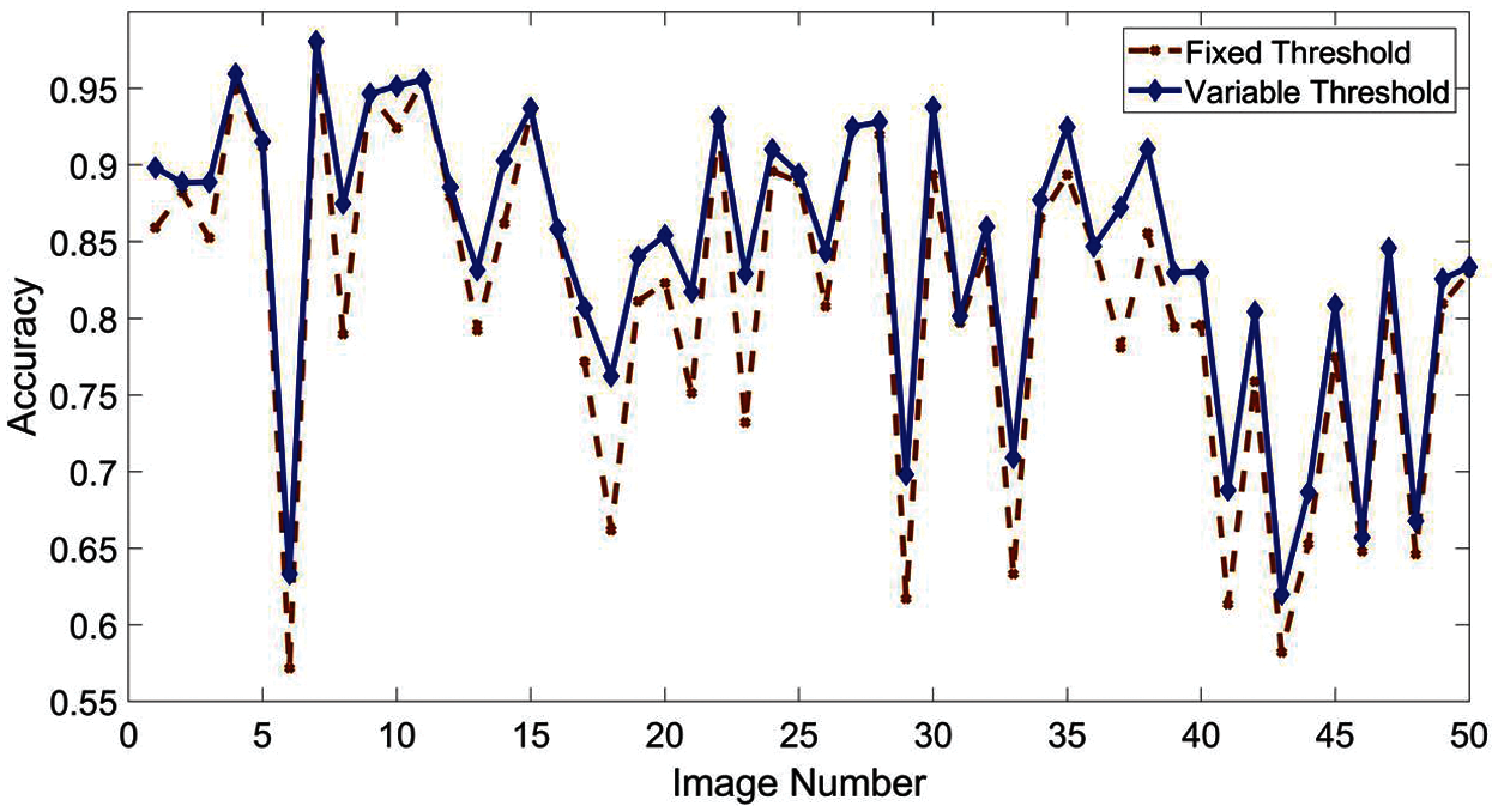
Figure 1: Accuracy evaluation of adaptive threshold i.e., the target threshold t used for training the model (blue solid line) and fixed threshold = 4 (brown dotted line) for first 50 images of dataset A

Figure 2: Block diagram of the proposed method for blur detection

Figure 3: Block diagram of the adaptive threshold prediction model

2.2.1 Data Preparation

In data preparation, first, we create a set of useful features. There is a variety of options to choose sophisticated features in spatial and transform domains [24]. Further, the original features can be refined to get a more effective sub-feature vector. One of such techniques, discrimination power analysis (DPA) is presented in [24,25] to get more discriminated features. Thus, the model accuracy can vary by choosing the different features for learning. In the proposed method, we have computed a feature vector with ten well-known features (f1,f2,…,f10) without any further analysis. Detail of the features is given in Tab. 1.

Mean of all the pixels of an image contains the information about the total brightness. Standard deviation shows the amount of variation from the average value. A low standard deviation indicates that all the pixels tend to be very close to the mean value of pixels, whereas high standard deviation indicates that all the pixels are spread out over a large range. Median is a measure of an intensity level of the pixel which separates the higher intensity value pixels and lower intensity value pixels.

Covariance of an image is a measure of the directional relationship of the pixels. If the variables tend to show similar behavior, the covariance is a positive number, or negative in the opposite case. The correlation coefficient calculates the strength of the relationship between the pixels. The entropy measure calculates randomness among the pixels of an image. Skewness of the image contains information about the surface of the image. It is the measure of the asymmetry of the probability distribution of the pixels. Negative skew indicates that the bulk of the values lie to the right of the mean, whereas positive skewness indicates that bulk of the values lie to the left of the mean. Kurtosis gives information about the noise and resolution measurement together. Higher value of kurtosis indicates that noise and resolution are low. Contrast contains the distinguishable property of objects in an image. It is calculated by taking the difference between the maximum and minimum pixel intensity in an image. Energy gives information on directional changes in the intensity of the image.

We use images of dataset A to generate the data. In this way, for each image 1×10 dimensional feature vector f=(f1,f2,…,f10) is computed. To train a model, every feature vector f should have a target value, which is the best threshold for each image. Mathematically, training data can be represented as:

DT={f(i),t(i)}i=1,2,…,N1(1)

Here, N1 is the sample size of the training data. In our experiment total size of the training and testing data is N=N1+N2, where N2 is the sample size of the test data Dtest.

2.2.2 Model Learning

In this module, a classifier is evolved to solve a multiclass problem using support vector machine (SVM) binary learners. Multiple binary classifiers can be used to construct a multiclass classifier by decomposing the prediction into multiple binary decisions [26]. To decompose the binary classifier decision into one, we have used ‘onevsall’ coding type. Each class in the class set k is individually separable from all other classes. For each binary learner, one class is taken as positive, and the rest is taken as negative. This design uses all the combinations of positive classes for the binary learner. Non-linearity in the features is taken care of by kernel function by transforming nonlinear spaces into linear spaces. In our experiment, we have used ‘Gaussian’ as the kernel function. Training data DT is used to train an SVM multiclass classifier g^(f) for multiclass classification. The evolved classifier g^(f) takes the value of feature vector f of an image as input and classifies it into one of the nine classes i.e., (0,1,2,…,8).

2.2.3 Model Evaluation

Once the model g^(f) is trained with the training data DT, the assessment of learned model g^(f) is done with test data DTest. The mathematical expression for test data is given by:

DTest={f(i),t(i)}i=1,2,…,N2(2)

To evaluate the performance of the classifier, we compute classification loss (L). It is the weighted sum of misclassified observations and can be represented by the formula:

L=∑i=1N2wiI{t^var(i)−t(i)}(3)

Here, t^var is the threshold predicted by the classifier g^(f), t is the pre-known target value for test data and I{.} is the indicator function. In our experiment, the ratio of training data to test data is $9:1$. The model accuracy achieved with training data is 96.4%, and with test data, it is 87%.

2.3 LBP-Based Blur Measure

LBP [27] is one of the widely used methods for many computer vision problems, such as texture recognition [28], texture segmentation [29], image key point detection [30]. LBP has many different variants, like LBP histogram-based (LBP-B) [31], and pixel-wise LBP histogram-based (LBP-P) [32] approaches. Conventional LBP works by taking a window for each grayscale pixel ic. For each central pixel ic, the 8-bit binary number is generated, when ic is compared to each of its neighbors along the circle (8 neighbors for window of size 3×3) on its left-top, left-middle, left-bottom, right-top, etc. The LBP operator gives value 0 if ic is greater than its neighbor's value otherwise it gives 1. The LBP operator can be defined as:

LBPt,r=∑k=0t−1S(ik−ic)×2k(4)

S(v)={0,|v|<tfix1,|v|≥tfix(5)

where ic and ik are the intensity values of the central pixel and neighboring pixel located on the circular radius r at coordinate (xc,yc) and (xk,yk) respectively. tfix is the user defined small positive threshold to provide robustness against flat regions in image [32]. LBP responses oppositely to the noisy and blurred regions of the image. There is a tradeoff between sharpness sensitivity and noise robustness. In situations where high sensitivity to sharpness is needed, a discontinuity preserving noise reduction filter such as non-local means can be employed.

Yi et al. [21] proposed the LBP-based defocus blur where LBP patterns (8-bit) are reduced into only 10 patterns, out of which 9 patterns (denoted by 0−8) are of uniform, and all the non-uniform patterns are put into single bin denoted by 9. The uniform and non-uniform binary patterns are explained in [33]. Yi et al. [21] have observed that the bins 6, 7, 8 and 9 are prominently less populated in the blurred regions than that in the sharp regions. Hence, following formula is used to calculate the sharpness map of an image,

MLBP(x,y)=1K∑i=69(LBP8,1riu2)n(i)(x,y),(6)

where (LBP8,1riu2)n(i) is the number of rotation invariant of 8-bit LBP pattern, i is the bin position and K is the total number of pixels in the local region used to normalize the map.

2.4 Blur Classification

Once the classifier g^(f) is developed and evaluated from the above modules, threshold prediction becomes a simple and straightforward process. The feature vector of an image is provided to the classifier, and it returns an integer value for that image. The feature vector is classified into the range of 0−8 threshold value tvar. This tvar is then used as an input to the LBP process to generate the blur map MLBP. The output of the LBP is the grayscale image. After acquiring the initial blur map, pixels need to be declared sharp or blurred, and they need to be separated into blurred and sharp regions respectively. The blur map MLBP is now converted into binary image Mclassified with threshold Tseg given by formula,

Tseg=1H×W∑x,yMLBP(x,y)(7)

where H and W is the height and width of the retrieved blur map MLBP.

Mclassified(x,y)={0MLBP(x,y)<Tseg1otherwise(8)

3  Results and Discussion

3.1 Experimental Setup

In our experiments, we have used two datasets denoted as dataset A and dataset B. Dataset A is publicly available dataset [5] which consists of 704 defocus partially blurred images. This dataset contains a variety of images with different magnitudes of defocus blur and resolution, covering numerous attributes and scenarios, like nature, vehicles, mankind, and other living and non-living beings. Each image of this dataset is provided with a hand-segmented ground truth image indicating the blurred and non-blurred regions. Dataset B is a synthetic dataset which consists of 280 out of focus images from the dataset used in [34]. Each image of dataset B is synthetically generated by mixing the blur and focused part of other images. However, our ground truth segments the blur and non-blur regions, whereas the ground truth of dataset in [34] segments the defocus blur, motion blur, and non-blur regions. Three widely used criterion for the evaluation of a classifier are Accuracy, Precision, and F-measure.

3.2 Effectiveness of Variable Threshold

The idea of this work is based on the observation that the performance of LBP-based method is comparatively poor on some of the images. On analyzing the possible reasons for the low performance of LBP, we found that it has used a fixed threshold tfix for all the images as described in Eq. (5). Threshold prediction based on the type of image is the only and an important difference between the proposed method and the LBP, where LBP used a fixed threshold. Except threshold everything else used by the proposed method is the same as LBP till the generation of blur map. Fig. 4 shows the comparison of three thresholds for the first 100 images of the dataset A: (i) thresholds of the training data, (ii) fixed LBP thresholds, (iii) thresholds predicted by the model g^(f).

Adaptive threshold tfix is the appropriate choice as all the performance metrics show significant improvement as compared to fixed threshold. One such example is image number 18 of the dataset A. Fig. 5a shows the qualitative comparison using the blur maps of the image using adaptive and fixed threshold. In Fig. 5b, the quantitative comparison of proposed method is done with LBP with fixed threshold tfix=4. All the metrics (Accuracy, Precision, Recall, and F-measure) are improved when variable threshold is used. We can clearly infer from this figure that for image number 18 of the dataset A, variable threshold tvar=0 performed significantly better than the fixed threshold tfix=4. Hence, there is a scope for the performance improvement of LBP by adaptively changing the threshold.

3.3 Comparative Analysis

The proposed method is compared with five state-of-art methods, which are (a) LBP based segmentation defocus blur [21], (b) High frequency Discrete Cosine Transform (DCT) coefficients (HiFST) [6], (c) Histogram Entropy (HE) [35], (d) Discriminative blur detection features using Local Power Spectrum (LPS) [36], and (e) Discriminative blur detection feature using Kurtosis (LK) [5]. For comparisons, we have used two datasets, dataset A and the dataset B which are described in Section 3.1.

In the proposed method, each image is classified into sharp and blurred regions using the processes described in Section 2. Blur map MLBP is computed with a variable threshold tvar for each image. The sharpness map is scaled with the local window size of 15×15 pixels. The sharpness metrics of all comparative methods are the gray-scale images where the sharp region contains higher intensity pixels and blurred region has lower intensity pixels. Note that single window size w=15×15 is used in LBP with fixed threshold method as well as our proposed method. Binarization is the final step in the blur segmentation process which is achieved using Tseg.

Figure 4: True threshold (blue solid line), predictive threshold (green solid line), and the fixed threshold (red dotted line) for first 100 images from dataset A

Figure 5: Classified blur map using variable threshold (for this image) and fixed threshold (t=4) for the image number 18 from dataset A. (a) Classified blur maps, (b) Comparison based on accuracy, precision, and F-measure

To compare the performance of the operators quantitatively, we have shown the result of three evaluation measures as discussed in Section 3.1. Figs. 6a–6c show the respective comparison of Accuracy, Precision, and F-measure of our proposed method with five state-of-the-art methods using the first 100 images of the dataset A. Here, the graphs are highlighting two important points, (1) Most of the images give better Accuracy, Precision and F-measure using the predicted threshold than that of constant threshold of LBP and other 4 methods. (2) For the few images, the evaluation measures of the proposed method are lower than others. The main reason for the point (2) here is the loss of the trained model g^(f) which is 9% in our case which is described in Section 2.2.3. There is a possibility of biasing of the particular choice of images (i.e., scenario and degree of blurriness) with the blur measure operators. The evaluation performance of methods may differ as the test image differs. Therefore, quantitative analysis on some images would not qualify to compare the blur measure operator. There is also the possibility of model over-fitting of the trained model g^(f) since the model is trained on the dataset A. To outcast these limitations, we intend to run our quantitative analysis on (i) all 704 images of the dataset A. (ii) all 280 images of the dataset B. Fig. 7 shows the quantitative comparison of the proposed method with other methods on two different datasets. The performance metrics of dataset A are computed in Fig. 7a which clearly shows that the proposed method performs better than LBP with fixed threshold-based method, and other methods. To eliminate the prospect of model over-fitting, we also computed the performance metrics on the dataset B which is not used for training. Fig. 7b shows the performance metrics of dataset B. The performance of our proposed method is significantly higher when compared to other methods. Qualitative performance is also evaluated on the randomly picked images with different scenarios as well as the different degree of blur from both the datasets. All the methods are compared with the hand-labeled ground truth. Fig. 8 shows the blur maps of comparative methods using few images from dataset A. The blur map has higher intensity for the sharp region and lower intensity for the blurred region of the image. Fig. 9 shows the comparison of few more images from dataset A and B using classified map of all the methods. Both (a) and (b) subfigures clearly show that our proposed method can segment the blurred and sharp regions with higher accuracy regardless of the blur type and scenario. The performance of our method is better as compared to the LBP with a fixed threshold and other methods.

Figure 6: Comparison of the proposed method (green solid line) with state-of-the-art methods (LBP [21], HiFST [6], HE [35], LPS [36], LK [5]) for first 100 images from the dataset A based on: (a) Accuracy, (b) Precision, (c) F-measure

Figure 7: Comparison of the proposed method with state-of-the-art methods (LBP [21], HiFST [6], HE [35], LPS [36], LK [5]) based on accuracy, precision and F-measure using: (a) Dataset A with 704 images, and (b) Dataset B with 280 images

Figure 8: Blur maps achieved by different methods (proposed, LBP [21], HiFST [6], HE [35], LPS [36], LK [5]) for few images from dataset A

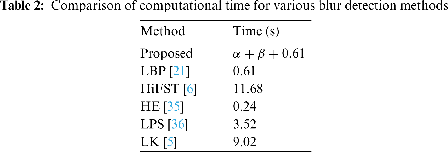
Tab. 2 shows the comparison of the average running times for randomly selected 100 images for various state-of-the-art methods. It is evident that the LBP method is the second most efficient among them. However, the proposed method takes some extra time as compared to the LBP as it computes the adaptive threshold before applying the LBP for computing blur map. Here α is the time for training the model for adaptive threshold and β=2.35 is the average time to calculate the threshold using the model. Thus, the proposed method is still efficient as compared to other methods except LBP, however, it improves the blur measure considerably as compared to LBP.

3.4 Limitations

In the proposed method, we have used simple set of features to learn the threshold. Though reasonable threshold values are obtained and final results are also upgraded, it may further be improved by replacing simple features with more sophisticated set of features from spatial and transform domains. Further, feature analysis and selection techniques can be applied to get specific and more effective set of features. Particularly, techniques including discrimination power analysis (DPA) and random projection (RP) [25,37] seem effective. In addition, we used SVM classifier to learn the model for threshold. Other machine and deep learning techniques can be applied and the results can be analyzed for prediction of a more accurate threshold. Further, it is observed that the LBP-based blur measure performs better for images with fewer objects and having homogeneous background, whereas its performance is deteriorated for images having multiple objects with heterogeneous background. In general, there is not any single blur measure that can perform well in all conditions. In our future study, we will consider these issues to achieve more accurate blur detection.

Figure 9: Final classified maps achieved by different methods (proposed, LBP [21], HiFST [6], HE [35], LPS [36], LK [5]) for few images; (a) from dataset A, (b) from dataset B

4  Conclusion

In this article, we have proposed an adaptive threshold-based method to improve the performance of the LBP method for blur detection. First, we trained a model using SVM which can predict the threshold based on the image features, and then respective thresholds are used to acquire the sharpness map of the images using LBP method. We have evaluated the performance of the proposed method in terms of Accuracy, Precision and F-measure using two benchmark datasets. The results show the effectiveness of the proposed method to achieve good performance over a wide range of images. Proposed method outperforms the state-of-the-art defocus segmentation methods.

Funding Statement: This work is supported by the BK-21 FOUR program and by the Creative Challenge Research Program (2021R1I1A1A01052521) through National Research Foundation of Korea (NRF) under Ministry of Education, Korea.

Conflicts of Interest: The authors declare that they have no conflicts of interest to report regarding the present study.

This work is licensed under a Creative Commons Attribution 4.0 International License, which permits unrestricted use, distribution, and reproduction in any medium, provided the original work is properly cited.