DOI:10.32604/cmc.2022.022085
| Computers, Materials & Continua DOI:10.32604/cmc.2022.022085 | |
| Article |
Software Defect Prediction Harnessing on Multi 1-Dimensional Convolutional Neural Network Structure
1Department of Information Systems, College of Computer and Information Sciences, Princess Nourah bint Abdulrahman University, Riyadh, Saudi Arabia
2Department of Computer Science and Information Technology, College of Community, Princess Nourah bint Abdulrahman University, Riyadh, Saudi Arabia
3College of Computing and Software Engineering, Kennesaw State University, Marietta, GA, 30060, USA
*Corresponding Author: Zuhaira Muhammad Zain. Email: zmzain@pnu.edu.sa
Received: 27 July 2021; Accepted: 16 September 2021
Abstract: Developing successful software with no defects is one of the main goals of software projects. In order to provide a software project with the anticipated software quality, the prediction of software defects plays a vital role. Machine learning, and particularly deep learning, have been advocated for predicting software defects, however both suffer from inadequate accuracy, overfitting, and complicated structure. In this paper, we aim to address such issues in predicting software defects. We propose a novel structure of 1-Dimensional Convolutional Neural Network (1D-CNN), a deep learning architecture to extract useful knowledge, identifying and modelling the knowledge in the data sequence, reduce overfitting, and finally, predict whether the units of code are defects prone. We design large-scale empirical studies to reveal the proposed model's effectiveness by comparing four established traditional machine learning baseline models and four state-of-the-art baselines in software defect prediction based on the NASA datasets. The experimental results demonstrate that in terms of f-measure, an optimal and modest 1D-CNN with a dropout layer outperforms baseline and state-of-the-art models by 66.79% and 23.88%, respectively, in ways that minimize overfitting and improving prediction performance for software defects. According to the results, 1D-CNN seems to be successful in predicting software defects and may be applied and adopted for a practical problem in software engineering. This, in turn, could lead to saving software development resources and producing more reliable software.
Keywords: Defects; software defect prediction; deep learning; convolutional neural network; machine learning
In recent years, software-run applications have become crucial in day-to-day human life. When COVID-19 embarked on the world in 2020, our dependency on software accelerated more due to the lockdown. Any slight disturbance or defect in any software could lead the working software to failure [1]. One of the preventive measures of software failure is to predict the software defect. A software defect is “an imperfection or deficiency in a work product where that work product does not meet its requirements or specifications and needs to be either repaired or replaced” [2]. It prevents the software from functioning as it plans and remains incompetent to the user's needs [3]. On the other hand, Software Defect Prediction (SDP) is a procedure to establish a model used in many projects to detect software errors. It classifies the software error as fault-prone and non-fault-prone. Hence, it helps the developer to find bugs in code. This procedure reduces the work in the maintenance phase and improves the quality of the software when deployed [4–8].
SDP offers exceptional benefits (1) to discover problems or defects earlier based on previous projects. Generally, these previous projects may have similarities with the new project. On top of that, predicting the problems help to increase the new project or software reliability; (2) To discover several independent variables used in a model. This helps the software developer appropriately manage the software defects; (3) To manage the testing plan and prioritize the faulty classes. Nevertheless, the software tester able to use the testing plan efficiently. Overall, SDP ensures that resources are effectively used in software development, resulting in lower costs and shorter development times. As a result, it increases software quality [9,10].
Realizing the importance of SDP, researchers have proposed a number of solutions to predict defects in the software. One of the solutions is using a statistical model based on the regression or function-approximation problem analysis [11]. Unfortunately, such methods fail to achieve proficient performances. This is because, each software application has a unique architecture comprised of distinct function combinations, development teams, and third-party components. This in turn causes the software defect prediction produces an incorrect result. To address the complexity issue, machine learning techniques have been advocated for SDP.
Several machine learning algorithms [7,12–17] such as naïve Bayes [18], logistic regression [19], random forest [20], and support-vector machines [21] have been implemented for SDP. Nevertheless, these traditional classifiers are still far from adequate because their predictive accuracies did not differ significantly [22,23]. Besides, they also suffer from overfitting. Recently, because deep learning (DL) has been successfully used to solve problems in other fields such as image processing [24] and speech recognition [25], researchers have examined the utility of DL algorithms for defect prediction [26,27] and suggested that this approach promises to advance SDP. The most popular DL algorithm used in SDP is the convolutional neural network (CNN) [5,28–35].
Although CNN algorithms may be useful for SDP, however, they seem to be very complex and have an insufficient accuracy level. This issue might be because of the 2D structure that was originally constructed to work only with 2D data such as images and videos. Recently, [36] leveraged 2D CNNs into 1D CNNs to work on patient-specific ECG data. The empirical results show that 1D CNNs are beneficial and therefore superior to their 2D equivalents. It has also gained popularity due to its superior performance in structural health monitoring and structural damage detection [37], high power engine fault monitoring [38], and damage detection in bearings [39,40].
Yadav [41] introduced 1D CNN in SDP to extract important features in the model and used SVM to classify software as defective or not defective. Although the model's performance was excellent, however, 1D CNN was not applied as a classifier which may cause the complexity of the model. In addition, the study did not consider a dropout layer in the 1D CNN structure which may cause it suffers from overfitting.
Motivated by the success of 1D-CNN algorithms applied in the aforementioned studies, we proposed a novel structure of 1D-CNN in predicting software defects with the aim to increase the performance of SDP on nine NASA datasets. On top of that, another five CNN models with different structures were also built to investigate the impact of different architecture on the performance of CNN in SDP. This paper makes the following contributions:
• We propose a novel structure of 1D-CNN, a deep learning architecture to extract useful knowledge, identify and model the knowledge in the data sequence, reduce overfitting, and finally, predict whether the code units are defects prone.
• We investigate the impact of different architecture of 1D-CNN on SDP performance by developing five CNN models with five different structures in terms of the dropout layer, kernel size, filter size, and the inclusion of an additional convolutional layer, and type of convolutional and max-pooling layers. The empirical results show that adding a dropout layer to a 1D-CNN classifier can reduce overfitting and enhance the model's performance in predicting software defects. On the other hand, increasing the kernel size of the proposed 1D-CNN model, reduces the filter size, adds an additional convolutional layer, and uses 2D convolutional and max pooling layers do not have a great impact on the detection of software defects.
• We design large-scale empirical studies to present the effectiveness of the proposed model by making a comparison with four established traditional machine learning baseline models and four state-of-the-art baselines in SDP based on the NASA datasets [42]. Results show that the proposed 1D-CNN software defect classification model achieved superior performance.
• Finally, we present the optimal 1D-CNN model by tuning three hyperparameters (the number of epochs, learning rate, and dropout rate) of the proposed 1D-CNN model.
The following is the paper's organization. Section 2 reviews related work. Section 3 provides the materials and methods of the proposed model. Section 4 presents the results and discusses the stated research questions. Section 5 gives the threats to validity from the construct, external, and internal validity. Section 6 gives the conclusion, and summarizes the study and suggests possible future works.
Deep learning has been utilized in a variety of fields since 2012, including software engineering. Deep learning was first used in software defect prediction in 2015 [26], and since then, it has become more popular. Several studies have looked at the use of deep learning in software fault prediction up to now.
Yang et al. [26] developed a Deep Belief Networks (DBN) model that predicts defect-prone changes. They classified data using machine learning algorithms. Experiments demonstrate that their techniques can detect 32.22 percent more defects than the current state-of-the-art model [43]. Suggested using stacked denoising autoencoders (SDAE) to create valuable metrics from hand-crafted metrics in the NASA dataset, and they utilized ensemble algorithms to detect defects. The findings indicate that deep representations of current metrics are potentially beneficial for predicting software faults.
Wang et al. [4] utilized DBN to create new important features and machine learning models to classify defects in 2016. They demonstrated that their model surpassed state-of-the-art models in their tests. Li et al. [5] presented a CNN-based defect classifier that used feature extraction through CNN and classification via logistic regression in 2017. Their findings exceeded those obtained using DBN models [4]. In 2018, [44] predicted faults using a long-short term memory (LSTM) model. In the sequel, [45] predicted faults using tree-based LSTM models. Their findings, however, fall short of Li's model [5]. Pan et al. [31] enhanced Li's model in 2019 by increasing convolutional and maximum pooling layers. Additionally, they included a dropout layer to avoid overfitting and tuned hyperparameters to improve the proposed prediction model's accuracy.
Currently, Zhu et al. [46] improved the Whale Optimization Algorithm feature selection method, which uses metaheuristic search to pick less but closely related features. Additionally, they combined CNN and kernel extreme learning machines (KELM) to create a hybrid defect classifier that integrates the selected features into the abstract deep semantic features produced by CNN and boosts prediction performance by fully exploiting KELM's strong classification capability. Their findings established the advantages of the hybrid approach.
However, these methods used deep learning to extract novel characteristics and other machine learning techniques to classify software as defective or not defective. As a result, these methods continue to suffer from a complicated structure and inadequate accuracy in predicting software defects, which may be improved further. To address these problems, we propose a new deep learning model that simplifies the structure, reduces overfitting and improves accuracy. To conduct this study, we utilized a 1D-CNN method for predicting software defects. The next section details the whole procedure.
The dataset used in this study was collected by the NASA Metrics Data Program. It can be retrieved from [42]. This dataset has been cleaned by eliminating all redundant and inconsistent data. Nine datasets which have similar dependent variable (defects: [TRUE, FALSE]) were selected. The name, number of instances, and the number of features for each dataset are presented in Tab. 1. The cleaned NASA datasets consist of features that associate with software quality which is known as software metrics. The software metrics were categorized into four groups namely, line of codes (LOC), Halstead, McCabe, and count metrics. The software metrics for each dataset are presented in Tab. 2.
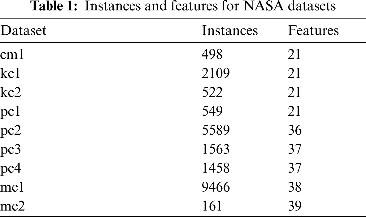
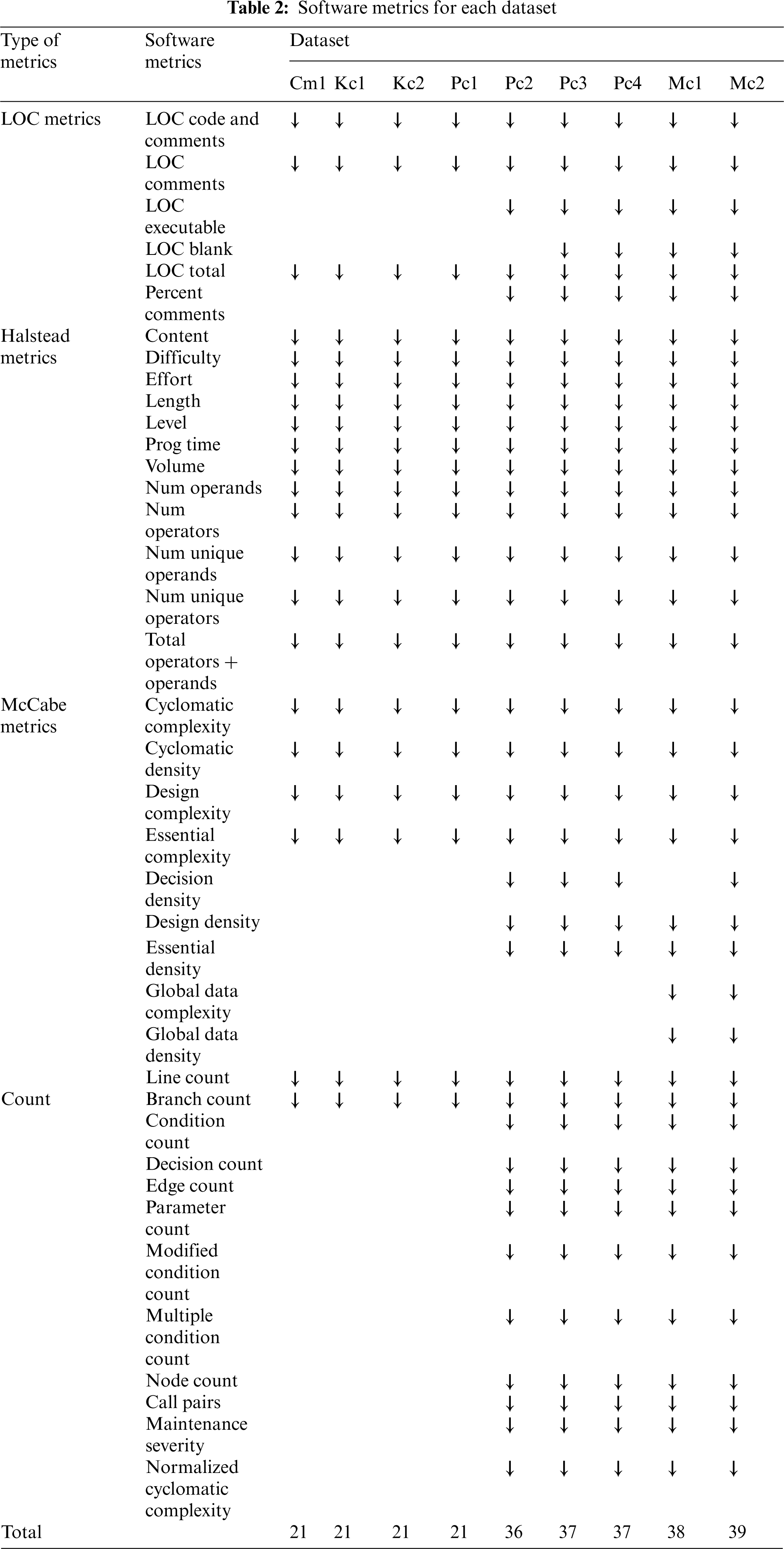
Fig. 1 shows the process of designing and developing the predictive models for this study.
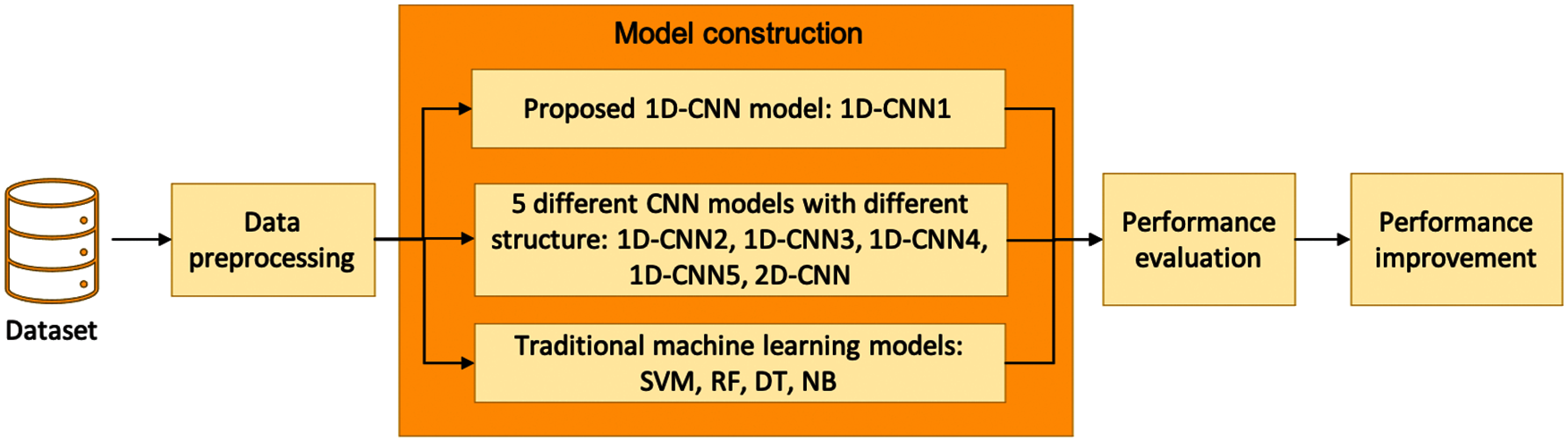
Figure 1: Method
Preprocessing of data is a crucial step to ensure that the data are of good quality. Normalization was applied to avoid the very large difference in feature values. In this analysis, the software metrics were scaled to an interval of [0, 1] using the Sklearn library MinMaxScaler function [47]. Since the data are considered small, they were then split into training and testing sets in a 65:35 ratio [48].
3.2.2 Software Defect Prediction Model Construction
In this phase, a structure for a 1D-CNN model was proposed as a baseline. Then, to investigate the impact of different structures on the performance of the proposed model, another five CNN models with different structures in terms of dropout layer exclusion, kernel size, filter size, the inclusion of an additional convolutional layer, and type of convolutional and max pooling layers were constructed. After that, four machine learning models were developed to measure the efficiency of our proposed model compared to the established machine learning models.
A deep learning architecture called 1D-CNN was proposed to extract useful knowledge, identifying and modelling the knowledge in the data sequence, and finally predict whether the unit of code is defect prone. The 1D-CNN consists of 2 main layers, convolutional and pooling layers.
Convolutional and pooling layers [49] are specifically built data preprocessing layers that have the task of filtering incoming data and extracting valuable information that will be utilized as an input on a fully connected network layer. Convolutional layers perform convolution operations on raw input data using convolution kernels to generate new feature values. Because this method was initially designed to extract features from image datasets, the input data must be in the form of a structured matrix [24]. The convolution kernel (filter) may be thought of as a small window (in comparison to the input matrix) that includes coefficient values in the form of a matrix. This window “slides” over the input matrix, performing convolution on each subregion (patch) that this defined window “meets”. These procedures result in a convolved matrix representing a feature value given by the coefficient values and dimension size of the applied filter. By applying alternative convolution kernels to the input data, numerous convolved features may be created that are typically more valuable than the input data's original initial features, therefore improving the model's performance.
The convolutional layers are normally preceded by a nonlinear activation function and then a pooling layer. A pooling layer is a method for subsampling that extracts specific values from the convolved features and provides a matrix with a reduced dimension. Like the convolutional layer, the pooling layer employs a small sliding window that accepts the values of each patch of the convolved features as input and outputs one new value that is described by an operation that the pooling layer is defined to accomplish. Max pooling and average pooling, for example, compute the maximum and average value of each patch's values. Consequently, the pooling layer generates new matrices that can be thought of as summarized versions of the convolved features generated by the convolutional layer. Because slight changes in the input do not affect the pooled output values, the pooling procedure can assist the system to be more robust.
The structure of our proposed 1D-CNN is depicted in Fig. 2. A brief description for each layer is presented in the following:
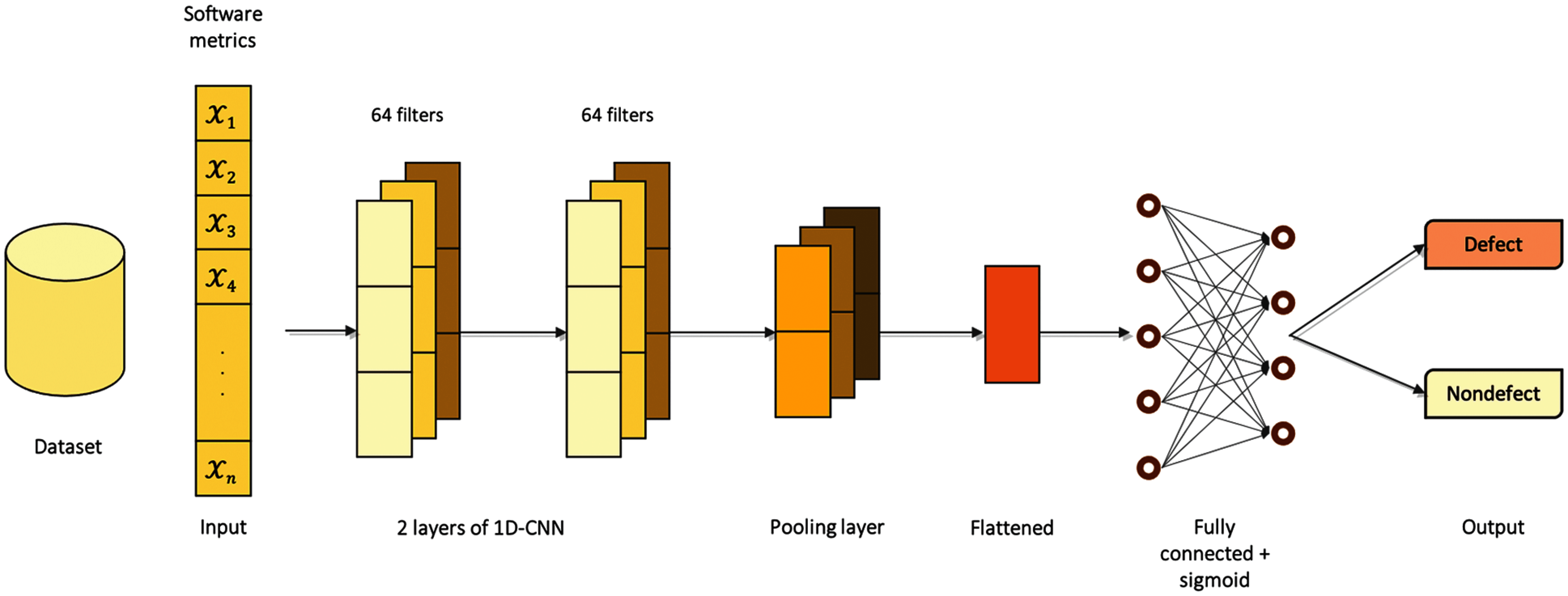
Figure 2: The architecture of the proposed 1D-CNN model
Input layer: Receive input of n number of features (software metrics). The value of n depends on the number of features in each dataset. For example, for CM1 dataset, the input layer receives 21 software metrics.
First Conv1D layer: The first convolutional layer reads across the input sequence and projects the results onto 64 feature maps with kernel size 1 and ReLU activation function. This layer generates convolved features which contain more knowledge and are more valuable than the original initial features of the input data.
Second Conv1D layer: The second performs the same operation on the 64 feature maps with kernel size 1 and ReLU activation function created by the first layer, attempting to amplify any salient features.
Max pooling layer: The feature maps were simplified by the max pooling layer with pool size 1. This layer extracts specific values from the convolved features and produces a matrix with a reduced dimension.
Dropout layer: This layer was added to the network to prevent the model from overfitting. Because the outputs of a dropout layer are randomly subsampled, the capacity or thinning of the network during training is reduced. As a result, a larger network, i.e., more nodes, may be required when using dropout.
Flatten layer: The distilled feature maps after the dropout layer were flattened into one long vector that can be used as input to the decoding process.
Fully connected layer: The fully connected layer consists of 2 dense layers with the last layer with sigmoid activation function was used to interpret each vector in the output sequence before the final output layer. The network used Adam optimization and the categorical cross-entropy as loss function, which is well known for learning a classification problem.
Output layer: The unit of code was classified whether it is defect-prone or not.
The proposed model was named 1D-CNN1. We also built another five CNN models with different structures (Tab. 3) to study the impact of different architecture on the performance of CNN and they were named 1D-CNN2, 1D-CNN3, 1D-CNN4, 1D-CNN5, and 2D-CNN.
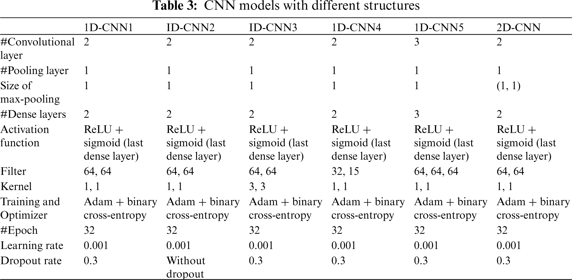
1D-CNN2: The structure is similar to 1D-CNN1 but without the dropout layer. This model construction aimed to investigate the impact of applying the dropout layer in the 1D-CNN structure on its performance.
1D-CNN3: The structure is similar to 1D-CNN1 except we change the kernel size for each convolutional layer to a standard practice size 3. This model was built to investigate the impact of kernel size on the performance of the 1D-CNN. We conducted additional experiments on the kernel size from 1 to 5.
1D-CNN4: The structure is similar to 1D-CNN1 except we change the filter size for each convolutional layer to a standard practice combination of 32 and 15, respectively. This model was constructed to explore the impact of using a smaller filter size on the performance of the proposed 1D-CNN model.
1D-CNN5: This model has an additional convolutional with a filter size of 64 for each layer. This model was developed to study the impact of adding an additional convolutional layer to the performance of the proposed 1D-CNN model.
2D-CNN: This model has a similar structure as 1D-CNN1 but in 2D convolutional and max pooling layers. This model was built to examine the impact of using 2D convolutional and max pooling layers on the performance of the proposed 1D-CNN model.
Traditional Machine Learning Models
Four popular machine learning models were also constructed to evaluate how good is our proposed model compared to these established models. A brief description of each machine learning technique was presented in the following.
Support Vector Machine (SVM): SVMs are statistical and machine-learning approaches that are used to predict outcomes. They are comparable to Gaussian, logistic, and multinomial regression in that they can be adopted to continuous, binary, and categorical outcomes. The details of the SVM algorithm can be found in the literature [50].
Random Forests (RF): RF are an extension of bagged decision trees. Samples are taken with the replacement of the training dataset, but the trees are designed in a way that decreases the association between individual classifiers. Specifically, for each split, instead of greedily selecting the best split point in the tree construction, only a random subset of features is considered. The details of the random forests algorithm can be found in the literature [20].
Decision Tree (DT): The DT methodology is a frequently used data mining technique for constructing classification systems based on various covariates or predictive algorithms for a target variable. This classification technique divides a population into branch-like segments that form an inverted tree with a root node, internal nodes, and leaf nodes. The technique is non-parametric, which enables it to efficiently handle huge, complex datasets without imposing a complex parametric framework. The details of the random forests algorithm can be found in the literature [51].
Naïve Bayes (NB): NB is among the purest subtypes of Bayesian type. This algorithm is based on the value of the conditional independence and all the independent attributes assigned to it. The naive bayes algorithm constructs its learning model using the collection of conditional independences and the dataset's frequency. NB is known for its simplicity and outstanding classification processes. The details of the random forest's algorithm can be found in the literature [52].
In this phase, the proposed model and the other 4 CNN models were implemented based on the structure and parameters described in subsection 3.2.2 using Keras from the TensorFlow library. The baseline models were implemented by setting their parameters to their default values using sklearn library. The experiment was conducted 5 times for each dataset, taking into consideration the occurrence of randomness. The performance of each model on each dataset was then measured in terms of accuracy, f-measure, training, and testing time. The average for each performance metric was computed and compared to find out which model has the highest performance in detecting software defects. According to the confusion matrix, which is presented in Tab. 4, the metrics are defined as follows.
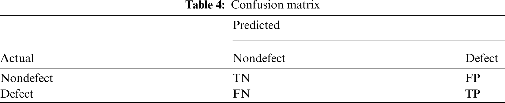
TP = True positive: If a defect subject is correctly classified as a defect
TN = True negative: If a nondefect subject is correctly classified as a nondefect
FP = False positive: If a nondefect subject is misclassified as a defect
FN = False negative: If a defect subject is misclassified as a nondefect
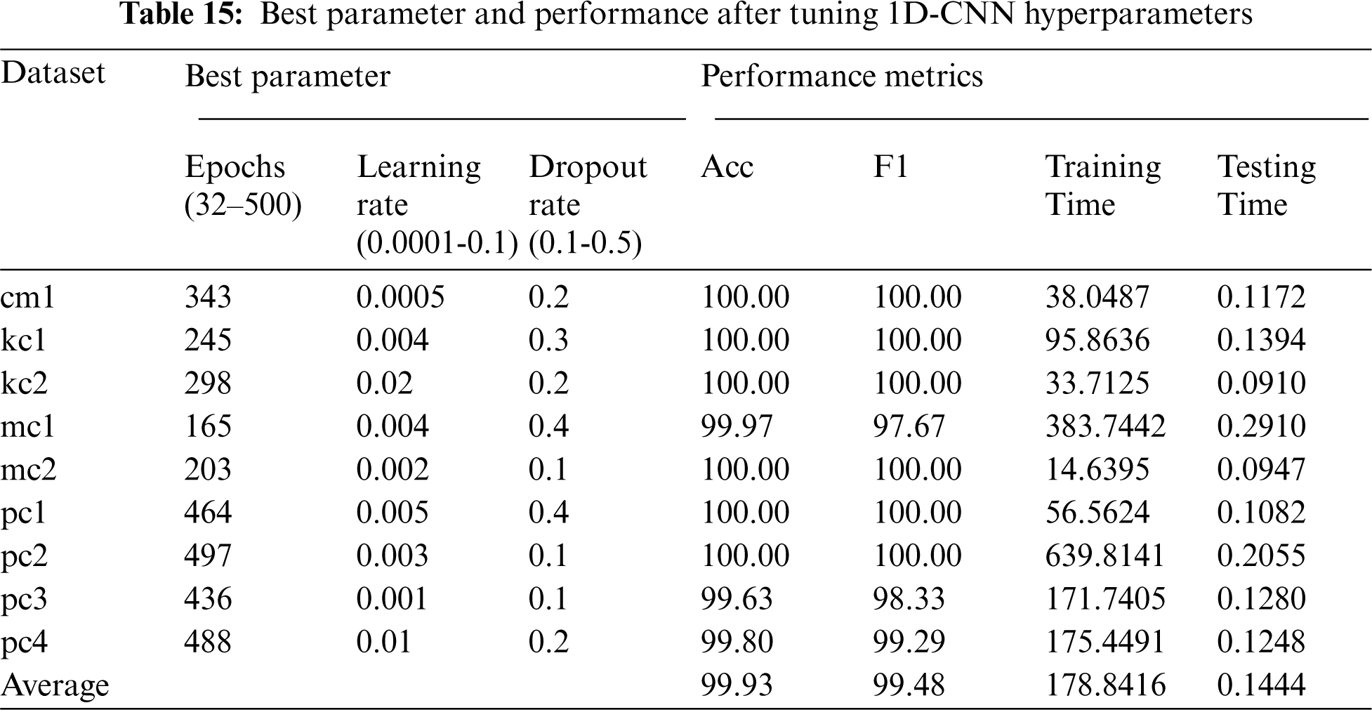
In this phase, the accuracy of the proposed model was improved by tuning three hyperparameters: the number of epochs, learning rate, and dropout rate. The number of epochs was tuned from 32–500, the learning rate was tuned from 0.001–0.1, and the dropout rate was tuned from 0.1–0.5. The trial was performed 50 times. The hyperparameter tuning was conducted using the Optuna framework from the Python library. This hyperparameter tuning was run 9 times since we used 9 different datasets. The performance of the proposed model using the optimal parameters on each dataset was then measured in terms of accuracy, f-measure, training, and testing time. The average for each performance metric was computed then compared with the performance of the proposed model before tuning the hyperparameters to see its impact.
To guide us in evaluating the proposed model, the following research questions were constructed:
RQ1: How effective is the proposed model compared with the baseline models?
RQ2: How effective is the proposed model compared with the state-of-the-art models?
RQ3: What is the impact of using different structures on 1D-CNN performance?
RQ4: Does tuning the 1D-CNN hyperparameter increase the performance?
The answers for RQ1 – RQ4 are discussed separately in the following subsections.
4.1 RQ1: The Effectiveness of the Proposed Model Compared with the Baseline Models
Tabs. 5–8 present the comparison of the performance values between the proposed 1D-CNN model and 4 baseline classification models: SVM, RF, DT, and NB on each dataset. The best average performance value is highlighted in bold.
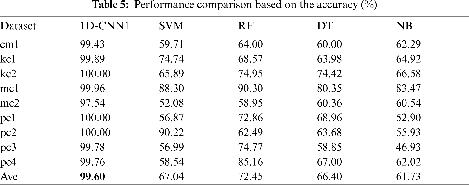
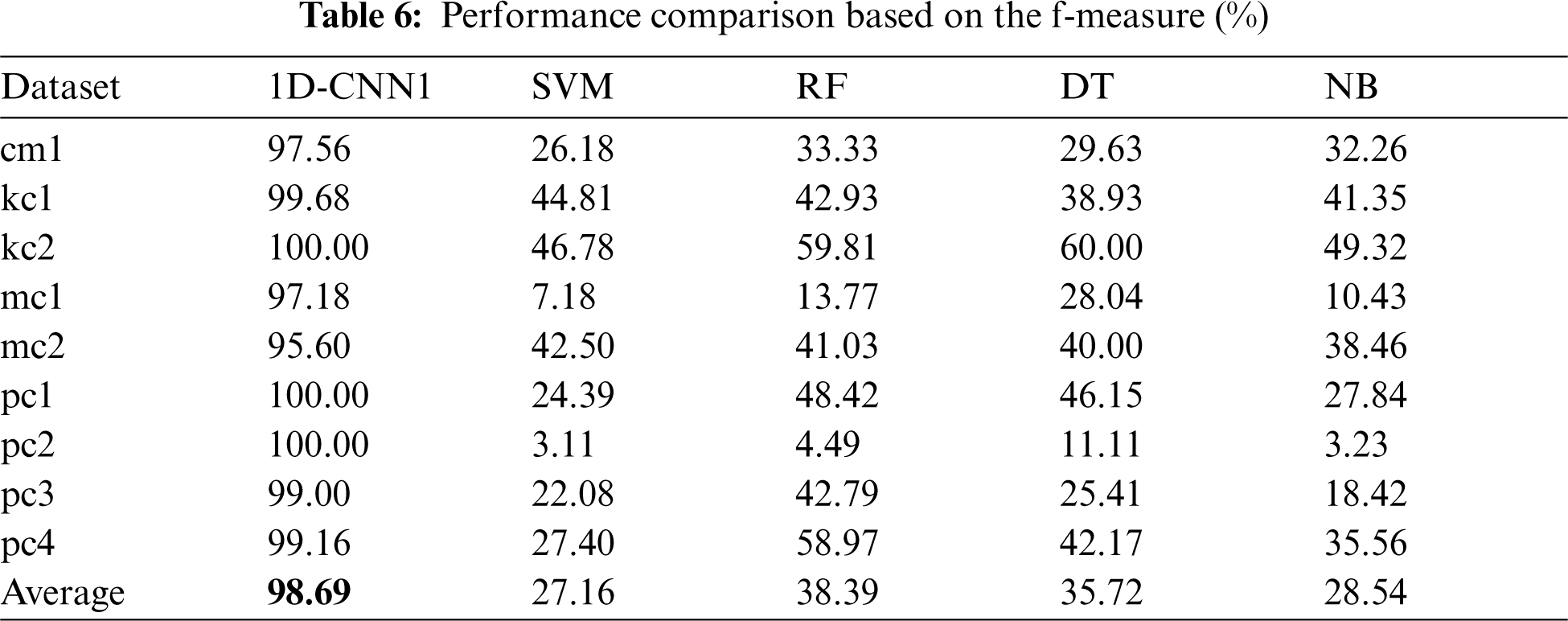
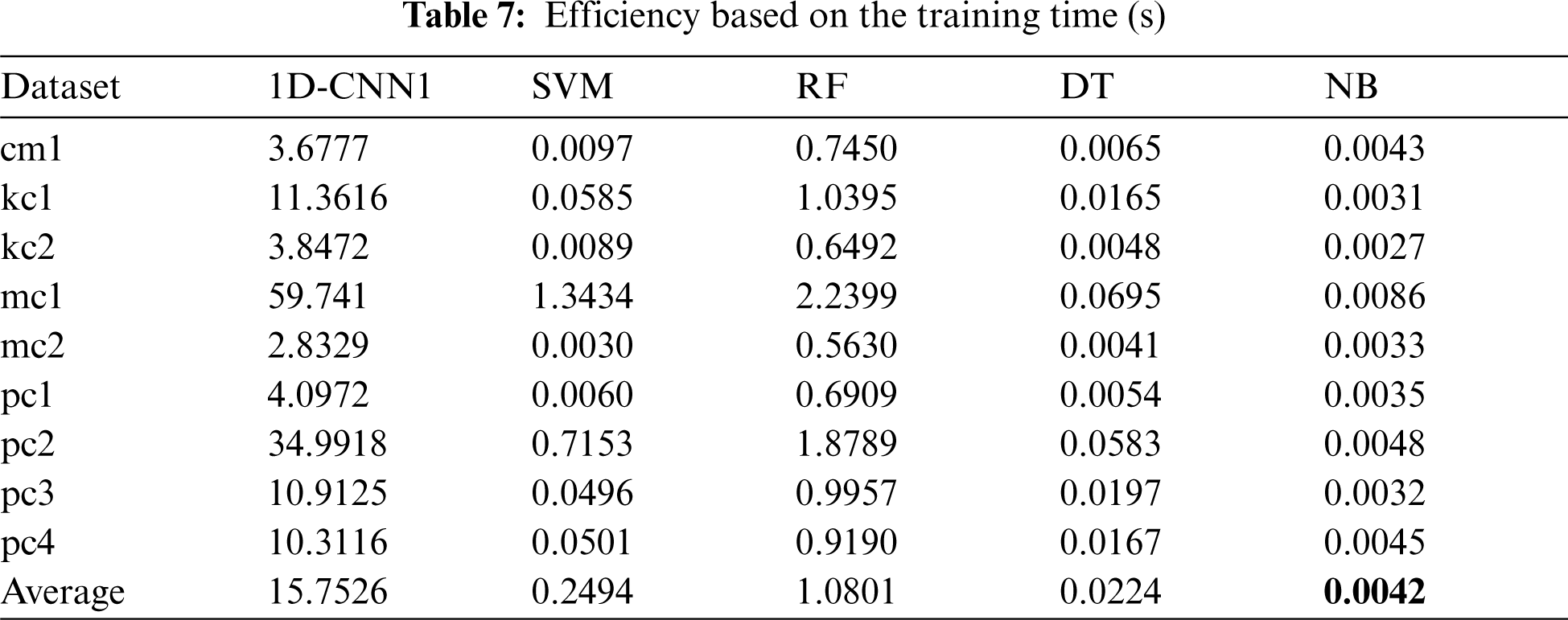
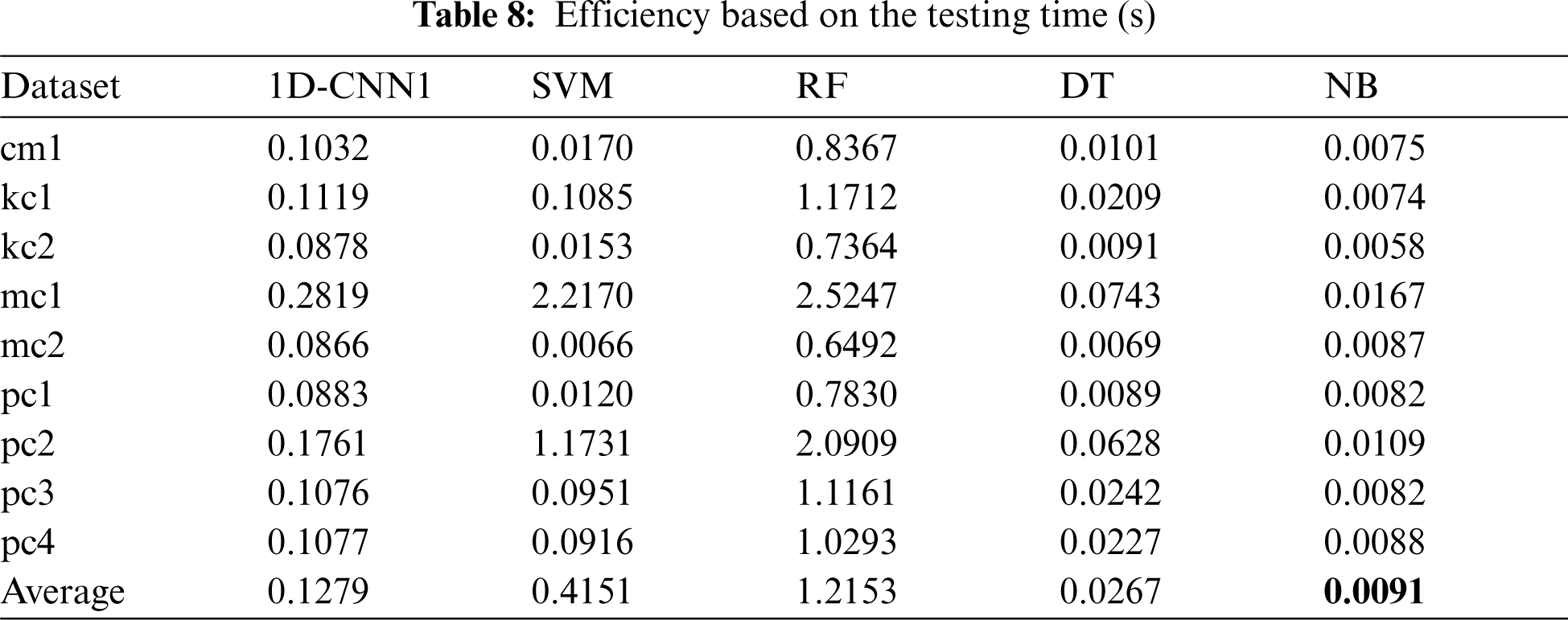
In terms of accuracy (Tab. 5), the proposed 1D-CNN model shows superiority compared to the four baseline models with 99.60%. In term of f-measure (Tab. 6), the proposed model again outperformed the baseline models with 98.69%. However, in terms of the training time (Tab. 7), the proposed model could not beat the baseline models. This is due to the deep network structure. Nevertheless, the training time of 15.7526 s is still considerable. Surprisingly, in terms of testing time (Tab. 8), the proposed model outperformed SVM and RF models but still cannot beat DT and NB. On average, the proposed model improved the accuracy and f-measure of the traditional machine learning models used in this study by 33% and 66%, respectively.
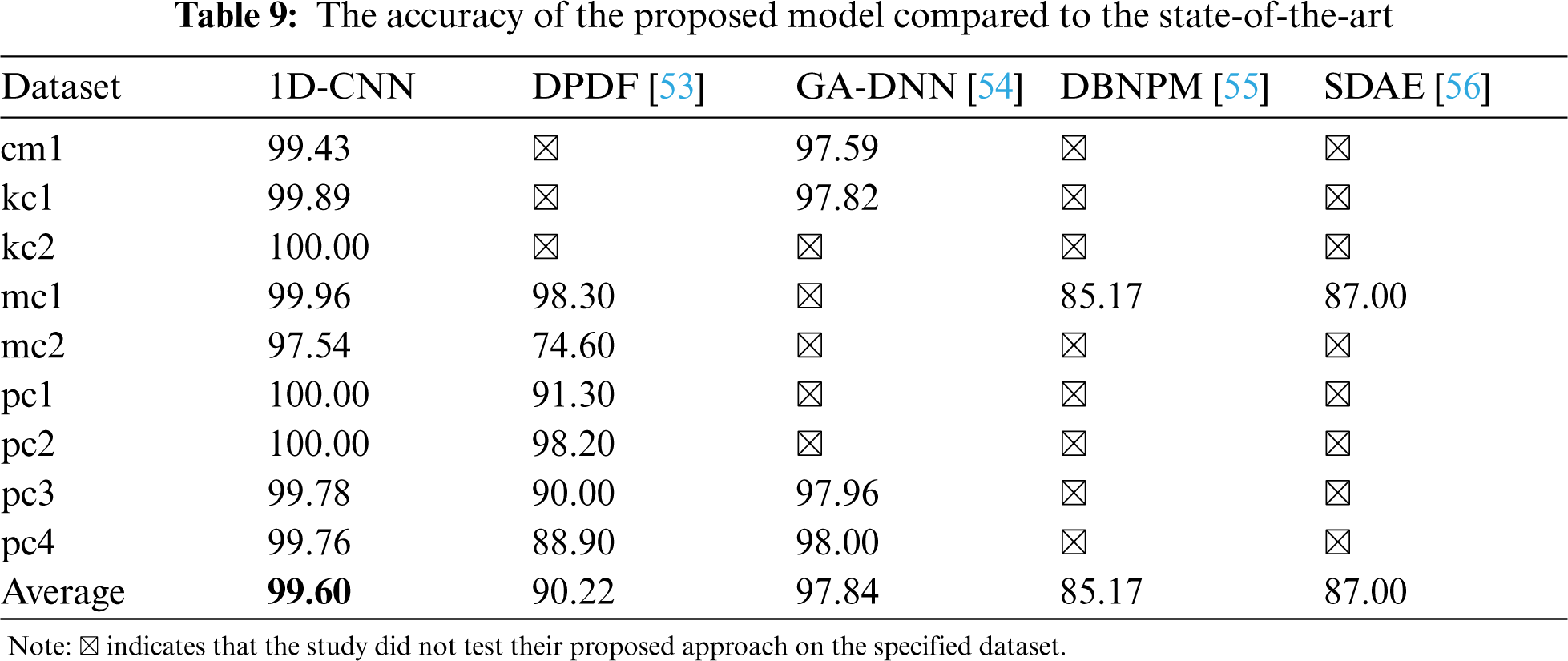
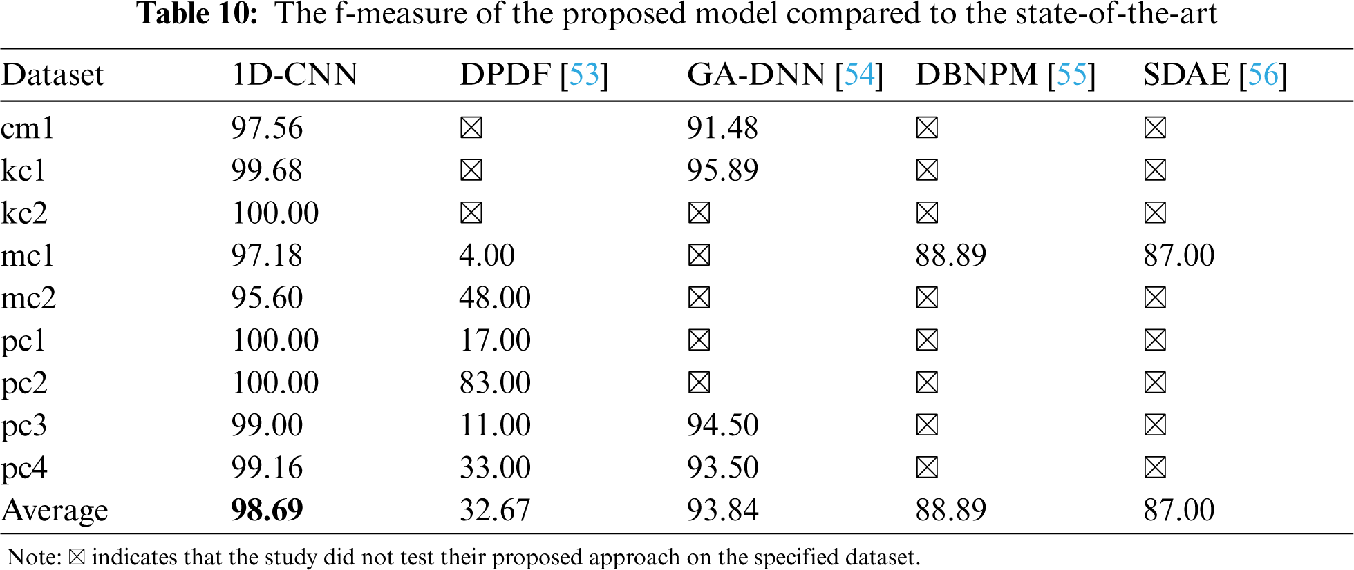
4.2 RQ2: The Performance of the Proposed Model Compared to the State-of-the-Art
To answer the second research question, we compare the performance of the proposed model with four state-of-the-art deep learning models: Defect Prediction with Deep Forest (DPDF) [53], Genetic Algorithm-Deep Neural Network (GA-DNN) [54], Deep Belief Network Prediction Model (DBNPM) [55], and Stack Denoising Auto-Encoder (SDAE) [56] and present the results in Tabs. 9 and 10. These studies were selected for using some similar datasets and performance measures. By comparison, our proposed model demonstrates greater performance in terms of classification accuracy and f-measure. The proposed 1D-CNN approach will have great potential in detecting software defects based on 9 NASA datasets.
4.3 RQ3: The Impact of Using Different Structures on 1D-CNN Performance
The effect of applying different structures on the performance of 1D-CNN algorithm in detecting software defects is discussed in this section.
Tabs. 11–14 presents the performance of 5 different CNN models compared to the proposed 1D-CNN model in terms of accuracy, f-measure, training, and testing time, respectively. It can be clearly seen that different structure gives a different value of performance to the CNN classifier on 9 different datasets.
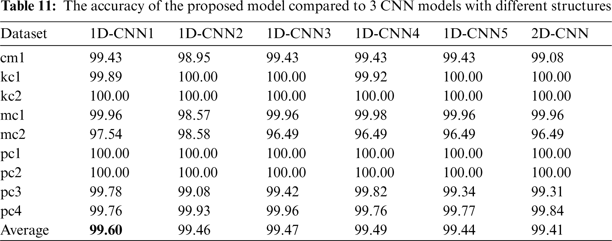
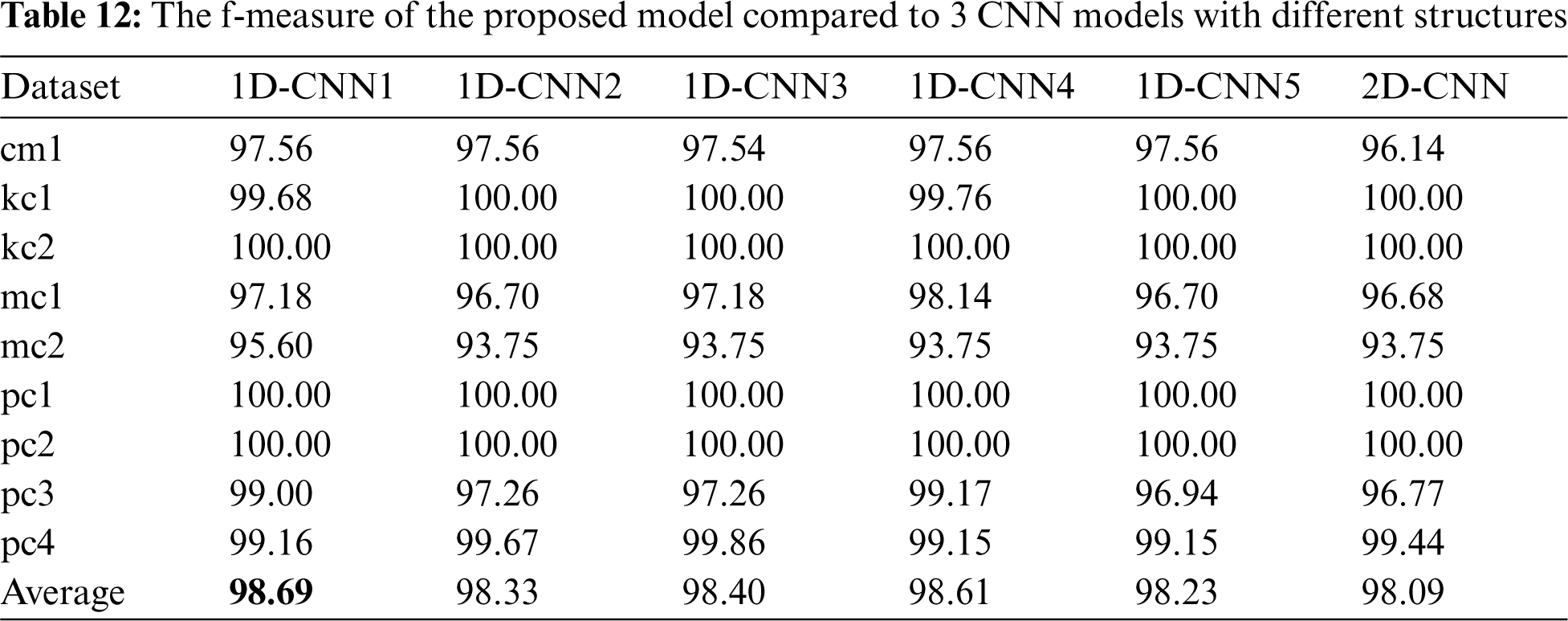

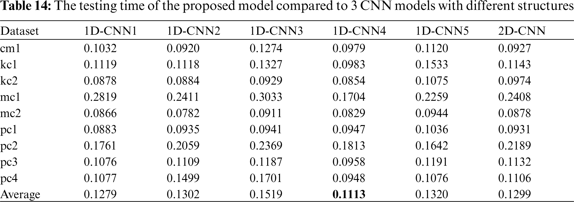
Compared to 1D-CNN2 which was omitted using the dropout layer, 1D-CNN1 shows a better performance in terms of accuracy and f-measure, and more efficient in terms of testing time. We can relate this result with the benefit of adding a dropout layer which can reduce overfitting in a classifier [57]. To visualize the impact of adding a dropout layer to the performance of the 1D-CNN classifier, we plotted the model training and testing error rate without (1D-CNN2) and with (1D-CNN1) dropout layer on each dataset in two separate graphs. Figs. 3–11 present the comparison on model loss without and with dropout layer on 9 datasets. For each figure, the graph on the left side is without a dropout layer while the one on the right side is with a dropout layer. A model that is underfitted will have a high training error but a low testing error, whereas a model that is overfitted will have a very low training error but a high testing error.
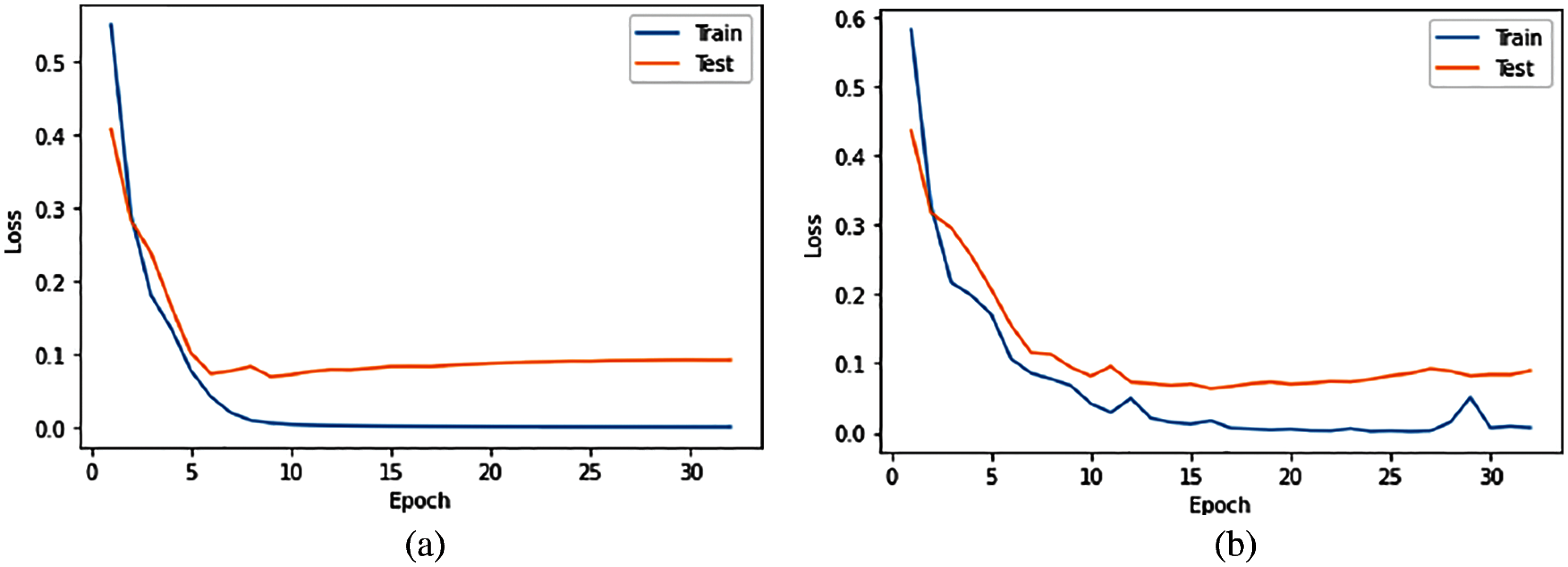
Figure 3: Comparison on model loss without and with dropout layer on CM1 dataset. a) 1D-CNN2, b) 1D-CNN1

Figure 4: Comparison on model loss without and with dropout layer on KC1 dataset. a) 1D-CNN2, b) 1D-CNN1

Figure 5: Comparison on model loss without and with dropout layer on KC2 dataset. a) 1D-CNN2, b) 1D-CNN1

Figure 6: Comparison on model loss without and with dropout layer on MC1 dataset. a) 1D-CNN2, b) 1D-CNN1

Figure 7: Comparison on model loss without and with dropout layer on MC2 dataset. a) 1D-CNN2, b) 1D-CNN1

Figure 8: Comparison on model loss without and with dropout layer on PC1 dataset. a) 1D-CNN2, b) 1D-CNN1

Figure 9: Comparison on model loss without and with dropout layer on PC2 dataset. a) 1D-CNN2, b) 1D-CNN1

Figure 10: Comparison on model loss without and with dropout layer on PC3 dataset. a) 1D-CNN2, b) 1D-CNN1

Figure 11: Comparison on model loss without and with dropout layer on PC4 dataset. a) 1D-CNN2, b) 1D-CNN1
Figs. 3–11 show that a dropout layer can help in reducing the testing error and can make the model more fit. We can conclude that adding a dropout layer to a 1D-CNN classifier can reduce overfitting, hence improve the performance of the model in predicting software defects.
Compared to 1D-CNN3, which used a larger kernel size (kernel size = 3), 1D-CNN1 still shows better performance and more efficient. To illustrate the impact of different kernel sizes on the performance of the CNN classifier, we run the experiment using kernel size from 1 to 5 on 9 datasets. The average for each performance metric was computed and visualized on bar graphs (Figs. 12–14). Fig. 12 shows that increasing kernel size does not improve the accuracy and f-measure value of the 1D-CNN classifier in software defect prediction. Figs. 13 and 14 illustrate that increasing the kernel size does not improve the efficiency of the 1D-CNN classifier in predicting software defects.
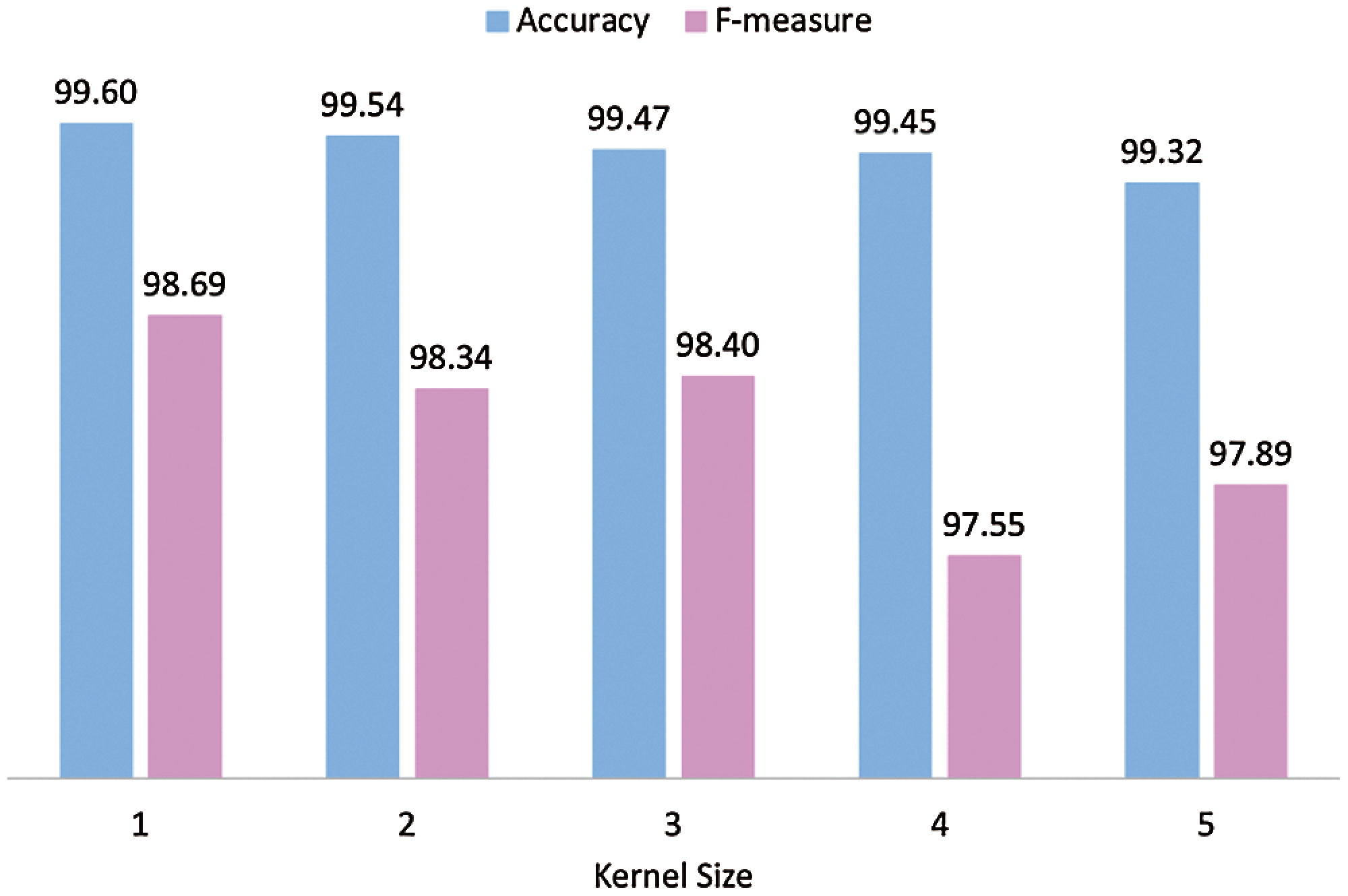
Figure 12: 1D-CNN model performance based on kernel size

Figure 13: 1D-CNN model training time (s) based on kernel size

Figure 14: 1D-CNN model testing time (s) based on kernel size
Compared to 1D-CNN4, which used a smaller filter size for each convolutional layer, 32 and 15, respectively, 1D-CNN1 has a better performance in terms of accuracy and f-measure. However, the 1D-CNN4 is more efficient in terms of training and testing time. One can argue that using a smaller filter size may increase the efficiency of a 1D-CNN classifier but do not improve its performance in predicting software defects.
Compared to 1D-CNN5, which used an additional convolutional layer, 1D-CNN1 shows better performance and more efficient. We can say that adding one convolutional layer could not improve the performance and efficiency of a 1D-CNN classifier in predicting software defects.
Compared to 2D-CNN, which used 2D convolutional and max pooling layers, 1D-CNN1 again shows a higher performance and more efficient in terms of testing time. In terms of accuracy and f-measure, all 1D-CNN models performed better that 2D-CNN model built in this study. One might argue that using 2D structure could not improve the performance of 1D structure in predicting software defect.
4.4 RQ4: The Impact of Tuning 1D-CNN Hyperparameters
The effect of applying hyperparameter tuning to the performance of 1D-CNN algorithm in detecting software defects is discussed in this section.
The optimal parameters and performance of 1D-CNN after conducting the hyperparameter tuning are shown in Tab. 15. It can be found that the set of optimal parameter values are different for each dataset. On average, the hyperparameter tuning increases the accuracy and f-measure of the proposed 1D-CNN model by 0.33% and 0.79%, respectively. However, as expected, the hyperparameter tuning does not improve the efficiency of the proposed model since the optimal number of epochs is larger than the number of epochs used in the proposed 1D-CNN model.
5.1 Threats to Construct Validity
The performance metrics used in our analysis relate to threats to construct validity. In this study, 4 evaluation metrics were selected: accuracy, f-measure, training, and testing time. Other measures, such as the kappa statistic, AUC, and MCC, can be used to evaluate binary classifiers. However, the 4 metrics selected in this study are widely used measures to evaluate the detection of software defects.
5.2 Threats to Internal Validity
The risks are primarily concerned with the unregulated internal variables that may affect the results of the experiment. The key internal threat is the possible faults during the implementation of our experiments. To reduce this hazard, we built six CNN classifiers obtained from Keras library and four baseline classifiers from sci-kit-learn libraries. We obtained the information on how to build 1D and 2D CNN models from Keras and TensorFlow documentation. The parameter setup for the proposed model is based on previous works that yield the best result. The default values obtained from the official sci-kit-learn documentation for the parameters for detecting software defects were adopted by four baseline classifiers.
5.3 Threats to External Validity
Threats to external validity relate to the possibility of generalizing our results. The experiments conducted in this study used nine NASA datasets. There are several datasets available such as PROMISE, Code4Bench, AEEEM, Relink, and CodeChef. Therefore, the experimental results might not be generalizable to other datasets, which might produce better or worse results for each software defect prediction model used in this study. However, the dataset we opted for is often used in previous software defect detection [53–56]. Different results can be generated by using different sets of software metrics.
In this study, a research method was designed to investigate the impact of different structures of the 1D-CNN classifier for the detection of software defects. The main process of the research method is to build the CNN models with different structures. First, we proposed a structure for a 1D-CNN model as a baseline. Second, we built another five CNN models with different structures in terms of dropout layer exclusion, kernel size, filter size, the inclusion of an additional convolutional layer, and type of convolutional and max pooling layers. Third, we developed four machine learning models to investigate how good is our proposed model compared to the established machine learning models. We evaluated the built models based on accuracy, f-measure, training, and testing time. The result was analysed and compared. Finally, we tuned three selected hyperparameters (the number of epochs, learning rate, and dropout rate) of the proposed 1D-CNN model to improve its performance.
The main result of this study reveals that compared to other CNN and traditional machine learning models, the proposed 1D-CNN software defect classification model achieved superior performance with 99.60% accuracy and 98.69% f-measure. This study also shows that adding a dropout layer to the proposed 1D-CNN structure improves its performance by reducing overfitting. It has a great impact on the discrimination between defect and nondefect software. On the contrary, increasing the kernel size of the proposed 1D-CNN model, reducing the filter size, adding an additional convolutional layer, and using 2D convolutional and max pooling layers do not have a great impact on the detection of software defects.
In addition, this study provides optimal values for the three selected hyperparameters for each dataset. We can conclude that conducting hyperparameter tuning improved the performance of the proposed 1D-CNN model in software defect prediction. According to these results, 1D-CNN appears to be effective for software defect prediction and can be applied for a practical challenge in the software engineering context. This in turn could lead to saving software development resources and producing more reliable software.
There are several ways to expand on this work. First, thorough experiments can be performed to investigate the impact of adding a number of convolutional layers in the model's overall performance. Second, some empirical studies can be conducted on different datasets or different levels of software defects. Third, other hyperparameters should be considered to be tuned to enhance the performance of the 1D-CNN model. Fourth, feature selection and imbalance issues in SDP should also be considered, which, in theory, might improve the performance of software defect prediction. Finally, experiments can be carried out to understand the success factors of 1D-CNN in different granularity levels of software defect such as change-level and file-level. This is particularly useful for practitioners, as it identifies situations in which 1D-CNN should be favored over alternative techniques.
CRediT authorship contribution statement: Zuhaira Muhammad Zain: Methodology, Data curation, Experiment, Formal analysis, Writing – original draft. Sapiah Sakri: Writing – Related work. Nurul Halimatul Asmak Ismail: Writing - Introduction. Reza M. Parizi: Writing – review and editing.
Acknowledgement: The authors would like to thank the Information Systems Department, College of Computer and Information Sciences, Princess Nourah bint Abdulrahman University for providing facilities to conduct the research.
Funding Statement: This research was funded by the Deanship of Scientific Research at Princess Nourah bint Abdulrahman University through the Fast-track Research Funding Program.
Conflicts of Interest: The authors declare that they have no conflicts of interest to report regarding the present study.
1. S. Omri and C. Sinz, “Deep learning for software defect prediction: A survey,” in Proc. ICSEW, Seoul, Korea, pp. 209–204, 2020. [Google Scholar]
2. ISDW Group, “IEEE standard classification for software anomalies,” IEEE Std 1044–2009 (Revision of IEEE Std 1044–1993), vol. 1044, no. 2, pp. 1–9, 2010. [Google Scholar]
3. Z. Miraj, “Software defect severity level prediction using machine learning techniques,” Ph.D. dissertation, Adama Science and Technology University, Ethiopia, 2021. [Google Scholar]
4. S. Wang, T. Liu and L. Tan, “Automatically learning semantic features for defect prediction,” in Proc. ICSE, New York, NY, USA, pp. 297–308, 2016. [Google Scholar]
5. J. Li, P. He, J. Zhu and M. R. Lyu, “Software defect prediction via convolutional neural network,” in Proc. QRS, Prague, Czech Republic, pp. 318–328, 2017. [Google Scholar]
6. P. S. Kumar, H. S. Behera, J. Nayak and B. Naik, “Bootstrap aggregation ensemble learning-based reliable approach for software defect prediction by using characterized code feature,” Innovations in Systems and Software Engineering, pp. 1–25, 2021. https://doi.org/10.1007/s11334-021-00399-2. [Google Scholar]
7. R. Malhotra, “A systematic review of machine learning techniques for software fault prediction,” Applied Soft Computing Journal, vol. 27, pp. 504–518, 2015. [Google Scholar]
8. E. N. Akimova, A. Y. Bersenev, A. A. Deikov, K. S. Kobylkin, A. V. Konygin et al., “A survey on software defect prediction using deep learning,” Mathematics, vol. 9, no. 11, 2021. [Google Scholar]
9. A. Joon, R. K. Tyagi and K. Chillar, “Literature review: Predicting faults in object-oriented software,” in Advances in Smart Communications and Imaging Systems: Select Proc. of MEdCom 2020, Singapore, Springer, pp. 309–323, 2021. [Google Scholar]
10. Y. Kamei and E. Shihab, “Defect prediction: Accomplishments and future challenges,” in Proc. SANER, Osaka, Japan, pp. 33–45, 2016. [Google Scholar]
11. T. M. Khoshgoftaar and K. Gao, “Count models for software quality estimation,” IEEE Transactions on Reliability, vol. 56, no. 2, pp. 212–222, 2007. [Google Scholar]
12. X. Jing, F. Wu, X. Dong, F. Qi and B. Xu, “Heterogeneous cross-company defect prediction by unified metric representation and CCA-based transfer learning,” in Proc. ESEC/FSE, New York, NY, USA, pp. 496–507, 2015. [Google Scholar]
13. X. Sun, T. Zhou, G. Li, J. Hu, H. Yang et al., “An empirical study on real bugs for machine learning programs,” in Proc. APSEC, 2018, Nanjing, China, pp. 348–357, 2017. [Google Scholar]
14. H. Lu, E. Kocaguneli and B. Cukic, “Defect prediction between software versions with active learning and dimensionality reduction,” in Proc. ISSRE, Naples, Italy, pp. 312–322, 2014. [Google Scholar]
15. T. Wang, Z. Zhang, X. Jing and L. Zhang, “Multiple kernel ensemble learning for software defect prediction,” Automated Software Engineering, vol. 23, no. 4, pp. 569–590, 2016. [Google Scholar]
16. Z. W. Zhang, X. Y. Jing and T. J. Wang, “Label propagation based semi-supervised learning for software defect prediction,” Automated Software Engineering, vol. 24, no. 1, pp. 47–69, 2017. [Google Scholar]
17. Z. Li, X. Y. Jing, X. Zhu and H. Zhang, “Heterogeneous defect prediction through multiple kernel learning and ensemble learning,” in Proc. ICSME, Shanghai, China, pp. 91–102, 2017. [Google Scholar]
18. P. Domingos and M. Pazzani, “On the optimality of the simple Bayesian classifier under zero-one loss,” Machine Learning, vol. 29, pp. 103–130, 1997. [Google Scholar]
19. D. R. Cox, “Two further applications of a model for binary regression,” Biometrika, vol. 45, no. 3/4, 1958. [Google Scholar]
20. L. Breiman, “Random forests,” Machine Learning, vol. 45, no. 1, pp. 5–32, 2001. [Google Scholar]
21. N. Cristianini and J. Shawe-Taylor, An Introduction to Support Vector Machines and other Kernel-Based Learning Methods, Cambridge, UK: Cambridge University Press, 2000. [Google Scholar]
22. S. Lessmann, B. Baesens, C. Mues and S. Pietsch, “Benchmarking classification models for software defect prediction: A proposed framework and novel findings,” IEEE Transactions on Software Engineering, vol. 34, no. 4, pp. 485–496, 2008. [Google Scholar]
23. B. Ghotra, S. McIntosh and A. E. Hassan, “Revisiting the impact of classification techniques on the performance of defect prediction models,” in Proc. ICSE vol. 1, Florence, Italy, pp. 789–800, 2015. [Google Scholar]
24. A. Krizhevsky, I. Sutskever and G. E. Hinton, “Imagenet classification with deep convolutional neural networks,” Communications of the ACM, vol. 60, no. 6, pp. 84–90, 2017. [Google Scholar]
25. G. Hinton, L. Deng, D. Yu, G. E. Dahl, A. Mohammed et al., “Deep neural networks for acoustic modeling in speech recognition: The shared views of four research groups,” IEEE Signal Processing Magazine, vol. 29, no. 6, pp. 82–97, 2012. [Google Scholar]
26. X. Yang, D. Lo, X. Xia, Y. Zhang and J. Sun, “Deep learning for just-in-time defect prediction,” in Proc. QRS, Vancouver, BC, Canada, pp. 17–26, 2015. [Google Scholar]
27. A. A. Saifan and N. al Smadi, “Source code-based defect prediction using deep learning and transfer learning,” Intelligent Data Analysis, vol. 23, no. 6, pp. 1243–1269, 2019. [Google Scholar]
28. J. Deng, L. Lu, S. Qiu and Y. Ou, “A suitable AST node granularity and multi-kernel transfer convolutional neural network for cross-project defect prediction,” IEEE Access, vol. 8, pp. 66647–66661, 2020. [Google Scholar]
29. L. Sheng, L. Lu and J. Lin, “An adversarial discriminative convolutional neural network for cross-project defect prediction,” IEEE Access, vol. 8, pp. 55241–55253, 2020. [Google Scholar]
30. S. Qiu, H. Xu, J. Deng, S. Jiang and L. Lu, “Transfer convolutional neural network for cross-project defect prediction,” Applied Sciences (Switzerland), vol. 9, no. 13, 2019. [Google Scholar]
31. C. Pan, M. Lu, B. Xu and H. Gao, “An improved CNN model for within-project software defect prediction,” Applied Sciences (Switzerland), vol. 9, no. 10, 2019. [Google Scholar]
32. X. Huo, Y. Yang, M. Li and D. C. Zhan, “Learning semantic features for software defect prediction by code comments embedding,” in Proc. ICDM, Singapore, pp. 1049–1054, 2018. [Google Scholar]
33. G. P. Bhandari and R. Gupta, “Measuring the fault predictability of software using deep learning techniques with software metrics,” Journal of Information Processing Systems, vol. 8, no. 2, pp. 241–262, 2018. [Google Scholar]
34. A. V. Phan, M. L. Nguyen and L. T. Bui, “Convolutional neural networks over control flow graphs for software defect prediction,” in Proc. ICTAI, Boston, MA, USA, pp. 45–52, 2017. [Google Scholar]
35. A. V. Phan and M. L. Nguyen, “Convolutional neural networks on assembly code for predicting software defects,” in Proc. IES, Hanoi, Vietnam, pp. 37–41, 2017. [Google Scholar]
36. S. Kiranyaz, T. Ince, R. Hamila and M. Gabbouj, “Convolutional neural networks for patient-specific ECG classification,” Annual International Conference of the IEEE Engineering in Medicine and Biology Society, vol. 2015, pp. 2608–2611, 2015. [Google Scholar]
37. O. Avci, O. Abdeljaber, S. Kiranyaz, M. Hussein and D. J. Inman, “Wireless and real-time structural damage detection: A novel decentralized method for wireless sensor networks,” Journal of Sound and Vibration, vol. 424, pp. 158–172, 2018. [Google Scholar]
38. T. Ince, S. Kiranyaz, L. Eren, M. Askar and M. Gabbouj, “Real-time motor fault detection by 1-d convolutional neural networks,” IEEE Transactions on Industrial Electronics, vol. 63, no. 11, pp. 7067–7075, 2016. [Google Scholar]
39. L. Eren, T. Ince and S. Kiranyaz, “A generic intelligent bearing fault diagnosis system using compact adaptive 1D CNN classifier,” Journal of Signal Processing Systems, vol. 91, no. 2, pp. 179–189, 2019. [Google Scholar]
40. W. Zhang, C. Li, G. Peng, Y. Chen and Z. Zhang, “A deep convolutional neural network with new training methods for bearing fault diagnosis under noisy environment and different working load,” Mechanical Systems and Signal Processing, vol. 100, pp. 439–453, 2018. [Google Scholar]
41. H. S. Yadav, “Increasing accuracy of software defect prediction using 1-dimensional CNN with SVM,” in Proc. INOCON, Bengaluru, India, pp. 1–6, 2020. [Google Scholar]
42. C. Tantithamthavorn, “NASA defect dataset,” 2016. Available: https://github.com/klainfo/NASADefectDataset. [Google Scholar]
43. H. Tong, B. Liu and S. Wang, “Software defect prediction using stacked denoising autoencoders and two-stage ensemble learning,” Information and Software Technology, vol. 96, pp. 94–111, 2018. [Google Scholar]
44. X. Zhang, K. Ben and J. Zeng, “Using cross-entropy value of code for better defect prediction,” International Journal of Performability Engineering, vol. 14, no. 9, pp. 2105–2115, 2018. [Google Scholar]
45. H. K. Dam, T. Pham, S. W. Ng, T. Tran, J. Grundy et al., “Lessons learned from using a deep tree-based model for software defect prediction in practice,” in Proc. MSR, Montreal, QC, Canada, pp. 46–57, 2019. [Google Scholar]
46. K. Zhu, S. Ying, N. Zhang and D. Zhu, “Software defect prediction based on enhanced metaheuristic feature selection optimization and a hybrid deep neural network,” Journal of Systems and Software, vol. 180, pp. 111026, 2021. [Google Scholar]
47. F. Pedregosa, G. Varoquaux, A. Gramfort, V. Michel, B. Thirion et al., “Scikit-learn: Machine learning in python,” Journal of Machine Learning Research, vol. 12, pp. 2825–2830, 2011. [Google Scholar]
48. P. Szczuko, M. Lech and A. Czyżewski, “Comparison of methods for real and imaginary motion classification from EEG signals,” Intelligent Methods and Big Data in Industrial Applications. Studies in Big Data, vol. 40, pp. 247–257, 2019. [Google Scholar]
49. W. Rawat and Z. Wang, “Deep convolutional neural networks for image classification: A comprehensive review,” Neural Computation, vol. 29, no. 9, pp. 2352–2449, 2017. [Google Scholar]
50. H. Drucker, C. J. C. Surges, L. Kaufman, A. Smolaf and V. Vapnik, “Support vector regression machines,” in Proc. NIPS, Denver, CO, USA, pp. 155–161, 1997. [Google Scholar]
51. L. Breiman, J. H. Friedman, R. A. Olshen and C. J. Stone, “Classification and Regression Trees,” Boca Raton: Routledge, 2017. [Google Scholar]
52. G. H. John and P. Langley, “Estimating continuous distributions in Bayesian classifiers,” in Proc. UAI, Montreal, QC, Canada, pp. 338–345, 1995. [Google Scholar]
53. T. Zhou, X. Sun, X. Xia, B. Li and X. Chen, “Improving defect prediction with deep forest,” Information and Software Technology, vol. 114, pp. 204–216, 2019. [Google Scholar]
54. C. Manjula and L. Florence, “Deep neural network based hybrid approach for software defect prediction using software metrics,” Cluster Computing, vol. 22, pp. 9847–9863, 2019. [Google Scholar]
55. H. Wei, C. Shan, C. Hu, Y. Zhang and X. Yu, “Software defect prediction via deep belief network,” Chinese Journal of Electronics, vol. 28, no. 5, pp. 925–932, 2019. [Google Scholar]
56. Y. Zhu, D. Yin, Y. Gan, L. Rui and G. Xia, “Software defect prediction model based on stacked denoising auto-encoder,” in Proc. AICON, Harbin, China, pp. 18–27, 2019. [Google Scholar]
57. N. Srivastava, G. Hinton, A. Krizhevsky, I. Sutskever and R. Salakhutdinov, “Dropout: A simple way to prevent neural networks from overfitting,” Journal of Machine Learning Research, vol. 15, no. 56, pp. 1929–1958, 2014. [Google Scholar]
 | This work is licensed under a Creative Commons Attribution 4.0 International License, which permits unrestricted use, distribution, and reproduction in any medium, provided the original work is properly cited. |