Computers, Materials & Continua DOI:10.32604/cmc.2022.021575
Article

Optimal Parameter Estimation of Transmission Line Using Chaotic Initialized Time-Varying PSO Algorithm

Abdullah Shoukat1, Muhammad Ali Mughal*,1, Saifullah Younus Gondal1, Farhana Umer2, Tahir Ejaz3 and Ashiq Hussain1

1Department of Electrical Engineering, HITEC University, Taxila, 47080, Pakistan
2Department of Electrical Engineering, Islamia University, Bahawalpur, 63100, Pakistan
3Department of Electrical Engineering, Iqra University, Islamabad, 44000, Pakistan
*Corresponding Author: Muhammad Ali Mughal. Email: ali.mughal@hitecuni.edu.pk
Received: 07 July 2021; Accepted: 26 August 2021

Abstract: Transmission line is a vital part of the power system that connects two major points, the generation, and the distribution. For an efficient design, stable control, and steady operation of the power system, adequate knowledge of the transmission line parameters resistance, inductance, capacitance, and conductance is of great importance. These parameters are essential for transmission network expansion planning in which a new parallel line is needed to be installed due to increased load demand or the overhead line is replaced with an underground cable. This paper presents a method to optimally estimate the parameters using the input-output quantities i.e., voltages, currents, and power factor of the transmission line. The equivalent π-network model is used and the terminal data i.e., sending-end and receiving-end quantities are assumed as available measured data. The parameter estimation problem is converted to an optimization problem by formulating an error-minimizing objective function. An improved particle swarm optimization (PSO) in terms of time-varying control parameters and chaos-based initialization is used to optimally estimate the line parameters. Two cases are considered for parameter estimation, the first case is when the line conductance is neglected and in the second case, the conductance is considered into account. The results obtained by the improved algorithm are compared with the standard version of the algorithm, firefly algorithm and artificial bee colony algorithm for 30 number of trials. It is concluded that the improved algorithm is tremendously sufficient in estimating the line parameters in both cases validated by low error values and statistical analysis, comparatively.

Keywords: Chaos; parameter estimation; transmission line; time-varying particle swarm optimization; pi-network

Nomenclature

1  Introduction

The major part of the power system consists of transmission lines which are the main medium of power flow between generation and distribution ends. The Loss of transmission lines means loss of power between two vital points which is not affordable at any cost. Long transmission lines are normally characterized by their line parameters such as series resistance, series reactance, shunt capacitance, and shunt conductance. The efficiency and reliability of the system are assured with continuous monitoring, protection, and control of the power system [1]. These parameters are very essential in determining the performance of the line, its analysis, and finding the location of the fault [2].

Therefore, accurate information of transmission line parameters and range of variations with boundary limits are of great importance to monitor the performance of the line and to design the protection schemes for fault conditions, these schemes can be fault location-based or current differential protection [3]. One method is to determine or estimate line impedance and admittance parameters from historical data [4], but the disadvantage of this method is that it does not presume real-time data of input and output variables; another approach is to identify parameters from input-output voltages, currents, powers and/or power factors measured at both ends of the transmission line [5]. Traditionally calculations of parameters were performed in offline mode using handbook-based formulas from tower geometry and properties of the conductor [6], these methods have many disadvantages as they do not incorporate short-term changes due to joule heating, ambient temperature variations which can contribute to incorrect operation of protection schemes. The transmission line parameters obtained from input-output measurements are also dependent on the time of measurement and weather conditions.

The paper provides a technique to accurately estimate transmission line parameters with minimum possible error and assumes that the input-output data of voltages, currents and power factor is available from measurement units at two ends of the line. This method considers distributed nature of the line parameters and estimates the per phase line parameters using the equivalent π-network model of the long transmission line. The input-output modeling used in this paper is based on the determination of the transmission line model from input-output measured/available data which is also known as the black-box approach [7]. In this paper set of nonlinear equations are used to determine transmission line parameters in which the validity of the model is not compared with linear equations, where a small change in operating conditions can change input-output parameters and lead to incorrect estimation of the line parameters. The input-output measurements of voltages, currents, and power factors are carried out by using synchronized phasor measurement units (PMUs) installed at both ends of the transmission line.

The PMUs are employed in the power system to measure magnitudes along with phase angles of voltages and currents at different locations [8,9], they also process the data acquired by digital recorders at substations. By using this measured input-output data the long transmission line, the line parameters from the set of nonlinear equations are then estimated. It is assumed that in absence of PMU the existing SCADA system employed at substations will perform measurements of voltages, currents, and power factor at both ends of the transmission line [10].

Recently, metaheuristic optimization algorithms have gained wide applications in solving complex, nonlinear engineering optimization problems [11] particularly in parameter estimation problems [12]. The metaheuristic algorithms are derivative-free algorithms compared to numerical optimization algorithms where a bad choice of initial solution can lead to diverging solutions instead of converging ones. Besides the many advantages associated with the metaheuristic algorithms, they suffer from premature convergence and trapping into a local optimal point problem [13]. The chaotic maps are bounded nonlinear deterministic systems that provide a way to generate initial population and updating control parameters of metaheuristic algorithms. The chaos search are also hybridized with metaheuristic algorithms to cope with the premature convergence problem. In literature there are many algorithms have been proposed for numerical function optimization that incorporate chaos theory to enhance performance in reaching the optimum solution [14–22].

In this paper long transmission line parameters estimation problem is formulated as an optimization problem and then solved using an improved particle swarm optimization (PSO) algorithm. The control parameters of the algorithm are made time-varying to achieve a dynamic behavior in achieving the global optimum and a chaos-based strategy is used to initialize the swarm of candidate solutions. The results obtained are then compared with the standard version of the algorithm, the firefly algorithm and the artificial bee colony algorithm in estimating the parameters of the transmission line model.

The paper is organized as follows, this Section is followed by Section 2 which presents the model of the transmission line and problem formulation, Section 3 outlines the optimization algorithms, Section 4 presents the simulation results and discussion whereas conclusions and references are provided at the end of the paper.

2  The Long Transmission Line Model and Problem Formulation

General equations representing long transmission line voltage and current are given in (1) and (2).

Vs=Vr.cos⁡hγl+Z∘.sin⁡hγl.Ir(1)

Is=Ir.cos⁡hγl+VrZ∘.sin⁡hγl(2)

where,

cos⁡hγl=(eγl+e−γl2)(3)

sin⁡hγl=(eγl−e−γl2)(4)

The characteristics impedance of the line [23] will be,

Z∘=r+jωlg+jωc(5)

For a lossless line, the characteristics impedance [23] will be,

Z∘=lc(6)

In case when the losses are neglected the above equation can be called as surge impedance or natural impedance equation of the line.

The equivalent pi network model of the transmission line [23] shown in Fig. 1 produces,

Vs=(1+ZY).Vr+Z.Ir(7)

Is=(2Y+ZY2).Vr+(1+ZY).Ir(8)

Figure 1: Equivalent π-network model of long transmission line

The impedance and admittance of the line is represented by (9) and (10).

Z=R+jX(9)

Y=G+jB(10)

Ir=Ir(cos⁡φr−jsinφr)(11)

From [23] comparing Eqs. (1) and (2) with (7) and (8), we get Z=Z∘.sin⁡hγl (12)

Y=1Z∘.tan⁡h(γl/2)(13)

In this paper, the data is used from [14] and assumed as available measured data of the long transmission line from measuring units at both ends of the line. Two different case studies of the line with conductance and without conductance are considered to estimate line parameters.

2.1 Transmission Line-Neglecting Shunt Conductance

The problem formulation uses the available data of voltages, currents, powers, power factors from [14], it is assumed that the data is coming from measurement units at both ends of the transmission line to estimate three unknown parameters R, X, and B as shown in the equivalent pi-network model of the long transmission line. In this case, the shunt conductance of the line is neglected. Taking Vr as a reference phasor, the two Eqs. (7) and (8) are separated into real and imaginary parts [23].

Vs(real)=Vr−BXVr+RIrcosφr+XIrsinφr(14)

a, say

Vs(img)=BRVr+XIrcosφr−RIrsinφr(15)

b, say

Combining real and imaginary parts, the sending end voltage equation will be represented by (16).

Vs=a+jb(16)

Is(real)=−RB2Vr+Ircosφr−XBIrcosφr−RBIrsinφr(17)

c, say

Is(img)=2BVr−XB2Vr−Irsinφr+RBIrcosφr+XBIrsinφr(18)

d, say

Is=c+jd(19)

It should be noted that the sending and receiving end power factor values are available from PMU or SCADA measurements at both ends of the transmission line. An error minimization objective function is formulated using Eqs. (17) and (19) to estimate unknown long transmission line parameters as expressed in (20).

e1=(|Vs,measured−Vs,estimated|)(20)

e2=(|Is,measured−Is,estimated|)(21)

AbsoluteError=e1+e2(22)

The per-unit values of line parameters R, L, and C are calculated by considering the equivalent circuit of the long transmission line as in [14] are given by Eqs. (25) and (26). The propagation constant per unit length is given as follows,

γ=α+jBl(23)

The characteristics impedance per unit length of the line will be,

Z∘=R+jXsin⁡hγl(24)

The per-unit impedance of the line along its length will be,

Z=Z∘γ(25)

The per-unit admittance of the line will be,

Y=YZ∘(26)

2.2 Transmission Line-Considering Shunt Conductance

Normally line losses are much greater than the insulation resistance of the line and the value of line conductance is very small. If due to environmental pollution and weather conditions the value of actual insulation resistance is very small, then the loss is represented by the conductance G in parallel with the capacitance of the line. The admittance of the line is given by Y= G + jB and the Eqs. (14), (15), (17) and (18) will be modified to consider the conductance of the line G, the real and imaginary parts of sending end voltage and currents are given as follows.

Vs(real)=Vr+RGVr−BXVr+RIrcosφr+XIrsinφr(27)

a, say

Vs(img)=XGVr+BRVr+XIrcosφr−RIrsinφr(28)

b, say

Is(real)=2GVr+RG2Vr−RB2Vr−2XGBVr+Ir cosφr−XBIr cosφr+RGIrcosφr+RBIr sinφr+XGIr sinφr(29)

c, say

Is(img)=2BVr+XG2Vr−XB2Vr+2RGBVr−Irsinφr−RGIrsinφr+XBIrsinφr+RBIrcosφr+XGIrcosφr(30)

d, say

By combining real and imaginary parts, we get the complete sending end voltage and current equations representing the π-model of the long transmission line model are given by (31) and (32).

Vs=a+jb(31)

Is=c+jd(32)

The above equations are used to estimate long transmission line parameters considering the shunt conductance of the line. From the equivalent circuit, the per-unit lengths of the line parameters R, L, C, and G are derived using the below equations.

cos⁡hγl=1+ZY(33)

=1+RG−XB+j(RB+XG)(34)

Suppose

cos⁡hγl=cos⁡h(α+jB)(35)

then,

cos⁡αcos⁡β=1+RG−XB(36)

sin⁡αsin⁡β=RB+XG(37)

Assigning

X1=1+RG−XB(38)

y1=RB+XG(39)

Eliminating α from (36) and (37), we get

cos2β= [ x1−(x12−4y12) ]2(40)

From (36), we get

cos⁡hα=y1/cos⁡β(41)

The per unit length values of the line parameters R, L, C, and G are obtained using (40) and (41).

3  Chaos Initialized Time-Varying PSO Algorithm (CITVPSO)

In this paper, an improved version of the particle swarm optimization algorithm, termed Chaos Initialized Time-Varying Particle Swarm Optimization (CITVPSO) is employed to estimate the parameters of the transmission line.

3.1 Particle Swarm Optimization (PSO)

The PSO is the most widely used swarm intelligence-based algorithm for engineering optimization problems. The algorithm simulates the food search behavior of birds. An optimization problem is formulated and optimized in terms of parameters update. In solving an optimization problem using the PSO algorithm; the candidate solution is termed as a particle. A group (swarm) of particles is employed to explore the problem search-space with the potential global solution. The PSO involves only two equations to be updated in each iteration, the velocity and position of the swarm of the particles expressed by (42) and (43)

vik+1=ωvik+c1r1(pBik−Xik)+c2r2(gBk−Xik)(42)

Xik+1=Xik+vik+1(43)

In (42) and (43), vi represents the velocity of particle i, k represents current iteration, ω represents inertia, c1 is a coefficient representing personal acceleration, c2 represents global acceleration coefficient, pB represents the personal best position of particle i in the current iteration, gB represents global best position among all particles achieved so far, r1 and r2 are two random numbers between 0 and 1, and Xi is particle's current position. The standard version of the algorithm is hereafter termed as the standard particle swarm optimization (SPSO) algorithm.

3.2 CITVPSO

In this work, a variant of PSO is proposed. The proposed variant differs from the standard PSO SPSO in terms of swarm initialization and algorithm parameters. In SPSO the particles are initialized randomly following a normal distribution whereas in the used variant the particles are initialized using a one-dimensional chaotic map and in the SPSO the algorithm parameters (ω,c1,c2) are assigned constant values throughout the iterations whereas in the proposed variant the parameters are made time-varying [24,25] to achieve good exploration and exploitation capabilities.

ωk=(ωmax.−ωmin.)×kmax.−kkmax.+ωmin.(44)

c1=(c1max.−c1min.)×kmax.−kkmax.+c1min.(45)

c2=(c2min.−c2max.)×kmax.−kkmax.+c2max.(46)

In (44)--(46), ωmax. and ωmin. denote maximum and minimum values of the inertia coefficient ω, respectively; c1max. and c1min. denote maximum and minimum values of the cognitive coefficient c1, respectively; c2max. and c2min. denote maximum and minimum values of the global coefficient c2, respectively. Whereas k represents current iteration and kmax. is the number of maximum iterations. The idea behind using the time-varying coefficients is to penalize the cognitive and global movements to facilitate global search in starting iterations and local search in the final iterations. This strategy provides a balance in exploring and exploiting the search space to find the global solution within some desired accuracy. The ω is varied between 0.4 and 0.9, c1 and c2 are varied between 0.5 and 2.5 in instances governed by current iteration and the maximum number of iterations as expressed in (44)–(46).

3.3 Chaos Initialization

Chaos can be termed as a bounded nonlinear system with deterministic nature having stochastic properties and much sensitivity to initial conditions and parameters [26]. Mathematically, chaos is deterministic and can be predicted because it is generated by iterating some deterministic equations, it is having a regularity parameter. Tent map is a one-dimensional chaos equation that has been used widely due to its advantages such as simple shape, higher iterative speed than other one-dimensional chaos maps like logistic map [26,27]. The equation for generating a tent map is expressed in (47); where z denotes the chaotic variable.

zn+1={2zn,znϵ(0,0.5)2(1−zn),znϵ(0.5,1)(47)

There is a limitation associated with the tent map that is due to the limitation of computer word length causing fractional parts of digits of floating-point numbers to be zero after a certain number of iterations. This makes the numbers to stuck at the fixed point 0 due to plunging at (0.2, 0.4, 0.6, 0.8) and some unstable points like (0, 0.5, 0.75) [17]. The solution to this problem is to provide a minor perturb when the chaos variable is stuck to the points stated above. The pseudo code for the tent map is provided below.

1: Begin

2: Initialize chaotic variables randomly

3: While (maximum iterations)

4: If the chaotic variable plunges

5: Provide a minor perturbation

6: Else

7: Update the variables by the Tent map equation

8: End

9: Next generation until maximum iterations

10: Scale the chaotic variables into the problem search space

11: End

The chaotic variables are generated in the range between 0 and 1 and then scaled into the problem search space using the relation expressed in (48).

X=Xmin.+(Xmax.−Xmin.)×z(48)

where X represents the parameter vector with dimensions (1×3) and (1×4) for case-1 and case-2, respectively. Whereas Xmin. and Xmax. represent minimum and maximum limits of the parameters respectively and z is the chaotic number.

The flow diagram of the CITVPSO is shown in Fig. 2.

Figure 2: Flow chart of CITVPSO

4  Results & Discussion

In this Section two case studies of long transmission lines are discussed, one without considering the conductance while in the other case shunt conductance is taken into consideration for estimation of line parameters. To make a fair comparison all the algorithms are tested for the same swarm size and 30 trial runs in estimating parameters in both the cases. The swarm size or population size is set as 100 for all algorithms. For SPSO ω, c1 and c2 are set as 0.9, 2, and 2, respectively. The maximum number of iterations is set as 500 for all the algorithms. For CITVPSO the parameter settings used are as stated before. The settings for FA and ABC algorithms are adopted from [28] and [29], respectively. The control parameters’ values are used in this paper are chosen based on personal experience and literature reviewed.

4.1 Case-I: Neglecting Shunt Conductance

A three-phase 220 kV overhead transmission line having a 300 km length, and frequency of 60 Hz, is considered. The per phase, per meter actual π-model line parameters, are taken, as given in [14], the line is delivering a load of 135 MW (3-φ) and 5.7 MVAr (3-φ). Considering Vr (receiving end voltage) as the reference phasor. The following quantities in Tab. 1 are assumed to be available data. To test the algorithms a wide parameter limit is used as given in (49) for case-I.

{10≤R≤500≤L≤10≤C≤5(49)

The actual and estimated values of the parameters R, L, and C using the CITVPSO algorithm are tabulated in Tab. 2. The table also gives the percentage error between the actual and the estimated values. It can be seen that for the parameter R the percentage error is in the order of 10e−12 whereas for the parameters L and C it is in the order of 10e-3. A comparison of the CITVPSO, SPSO, FA and ABC algorithms in terms of four different statistical indicators, for 30 trial runs of each algorithm, is given in Tab. 3. It is evident from the table that the CITVPSO algorithm has outperformed the counterpart SPSO, FA and ABC algorithms by achieving almost consistent minimal objective values in each run. The CITVPSO algorithm achieved an average and standard deviation of the order of 10e-14 whereas in the competing algorithms the FA could only achieve an average and standard deviation values that is in the order of 10e-04. The SPSO and ABC are far behind in this comparison. In comparison, CTVPSO proved to be a better solution for parameter estimation of the π-model of a long transmission line without considering the conductance. The convergence of the CITVPSO algorithm for the best run is depicted in Fig. 3, the algorithm can converge to the optimal objective value in less than 50 iterations. The estimated parameters trajectories are shown in Fig. 4 along with the actual parameter values. The estimated parameters are precisely tracking the actual parameters in a less number of iterations.

4.2 Case-II: Considering the Shunt Conductance

The actual long transmission line is represented by considering the effect of conductance in parallel, though the effect is very small but cannot be neglected. A π-type underground cable is considered to have a unity power factor, supplying a load of 100 MW per phase at receiving end with a voltage of 345 kV, the length of the line is 15-mile (24.14 km). The cable data is given in [23] and assumed as available or measured data for the underground cable and is tabulated in Tab. 4.

Figure 3: Convergence curve for best trial run of CITVPSO for Case-I

Figure 4: Parameter trajectories along with actual parameters for Case-I

Assuming the above data as available/measured data of underground cable, the long transmission line parameters are estimated by considering the shunt conductance of the line. The parameters are presented in Tab. 4. The parameter limits for case-II are given in (50).

{0≤R≤50≤L≤0.50≤C≤50≤G≤10(50)

The parameters are estimated using the available data and the four optimization algorithms i.e., CITVPSO, SPSO, FA and ABC for 30 trial runs. It turned out that the CITVPSO has tremendous performance in estimating the parameter with very low objective values, consistent in all trial runs, as compared to the other three algorithms.

The actual and estimated parameters for the best run of the CITVPSO algorithm along with percentage error are shown in Table. The algorithm is capable of precisely estimating the parameter with a very low percentage error evident from Tab. 5. Fig. 5 shows the convergence curve for the best run of the CITVPSO algorithm. The algorithm converged in less than 215 iterations. Further, the parameter trajectories for the estimated parameters are plotted in Fig. 6 along with the actual parameter values. It is clearly visible that the estimated parameters precisely track the actual parameters in a very less number of iterations.

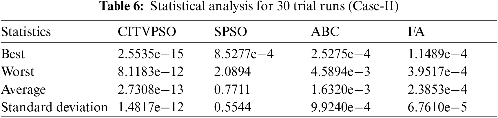
The statistics for the trial runs are presented in Tab. 6. The SPSO, FA and ABC lag behind the CITVPSO algorithm in all the statistical performance indicators and could only reach a best of order of 10e-4 in all the trial runs whereas the CITVPSO attained a best objective value of 2.5535e−15 which is far better than the values attained by the other three algorithms. The average and standard deviations of the SPSO, FA and ABC are too larger than the CITVPSO. Further, the global best achieved by all the algorithms in each trial run for both cases is given in Tab. A in Annexure.

Figure 5: Convergence curve for best trial run of CITVPSO for Case-II

Figure 6: Parameter trajectories along with actual parameters for Case-II

5  Conclusion

The paper presented an optimal method to estimate long transmission line parameters using input-output quantities i.e., voltages, currents, and/or power-factor measured at both ends of the transmission line. The measured data should be carefully recorded from measurement devices to avoid any error which will adversely affect the estimation process. An improved particle swarm optimization algorithm to avoid premature convergence and trapping in a local optimal is suggested. The control parameters of the PSO are made dynamic and the initialization is made chaotic to achieve better exploration and exploitation to support in finding the global solution. The performance of the algorithm is evaluated for two cases of parameter estimation: one case neglects the effects of conductance whereas in the other case the conductance is considered. The improved algorithm when compared with the standard version of the PSO algorithm, Firefly algorithm and Artificial bee colony algorithm, in the parameter estimation problem, turned out to be more effective and efficient indicated by the low percentage error values. The algorithm is tested for 30 trial runs and statistical analysis is performed for the trial runs. The statistical analysis revealed a superior performance of the improved algorithm over the standard PSO, firefly and artificial bee colony algorithms in terms of achieving low average and standard deviation values for the trial runs. The CITIVPSO achieved 1.7764e-14, 1.2022e-13, 2.1179e-14 and 1.8705e-14 best, worst, average and standard deviation values for Case-I respectively and 2.5535e-15, 8.1183e-12, 2.7308e-13 and 1.4817e-12 best, worst, average and standard deviation values for case-II respectively which is far better than the values achieved by the SPSO, FA and ABC algorithms. In this paper, the CITVPSO algorithm proved to be a good algorithm for the transmission line parameter estimation problem, comparatively. The method can be implemented to the real transmission line to evaluate the performance of the line, expansion of transmission line network in case of load growth, or when underground cable replaces the overhead lines and parameters of parallel lines or the cable are required to be determined. In future, other recent algorithms can be applied to this problem for comparison and any better performance.

Funding Statement: The authors received no specific funding for this project.

Conflicts of Interest: The authors declare that they have no conflicts of interest to report regarding the present study.

Annexure

This work is licensed under a Creative Commons Attribution 4.0 International License, which permits unrestricted use, distribution, and reproduction in any medium, provided the original work is properly cited.