DOI:10.32604/cmc.2022.021421
| Computers, Materials & Continua DOI:10.32604/cmc.2022.021421 | |
| Article |
Pseudo NLP Joint Spam Classification Technique for Big Data Cluster
1Department of Electrical and Computer Engineering, Sungkyunkwan University, Suwon, 16419, Korea
2Department of Computer Education, Sungkyunkwan University, Seoul, 03063, Korea
*Corresponding Author: Nawab Muhammad Faseeh Qureshi. Email: faseeh@skku.edu
Received: 02 July 2021; Accepted: 12 August 2021
Abstract: Spam mail classification considered complex and error-prone task in the distributed computing environment. There are various available spam mail classification approaches such as the naive Bayesian classifier, logistic regression and support vector machine and decision tree, recursive neural network, and long short-term memory algorithms. However, they do not consider the document when analyzing spam mail content. These approaches use the bag-of-words method, which analyzes a large amount of text data and classifies features with the help of term frequency-inverse document frequency. Because there are many words in a document, these approaches consume a massive amount of resources and become infeasible when performing classification on multiple associated mail documents together. Thus, spam mail is not classified fully, and these approaches remain with loopholes. Thus, we propose a term frequency topic inverse document frequency model that considers the meaning of text data in a larger semantic unit by applying weights based on the document’s topic. Moreover, the proposed approach reduces the scarcity problem through a frequency topic-inverse document frequency in singular value decomposition model. Our proposed approach also reduces the dimensionality, which ultimately increases the strength of document classification. Experimental evaluations show that the proposed approach classifies spam mail documents with higher accuracy using individual document-independent processing computation. Comparative evaluations show that the proposed approach performs better than the logistic regression model in the distributed computing environment, with higher document word frequencies of 97.05%, 99.17% and 96.59%.
Keywords: NLP; big data; machine learning; TFT-IDF; spam mail
Spam text messages and emails cause significant damage to message communication systems. “Among commercial emails intended for commercial purposes, spam emails that the recipient does not want are causing various harms, such as a decline in personal, domestic, and even national credibility [1].” “We find several spam mails such as pornographic, advertisements, bond prizes and online lottery, free illegal software, gambling, and letters of good luck [2].” “As Internet use increases, hacking and intrusion occur frequently, and government agencies, government offices, and operating systems are exposed to risk [3].” It is challenging for humans to identify and translate context, emotion, intent, or keywords, such as textual spam or search results. Special skills are required to detect essential parts, such as emotions and subjects. Natural language processing (NLP) provides a means for computers and humans to communicate. NLP can efficiently handle the analysis of patterns and structures in such text.
There are several document classification approaches to efficiently classify spam mail, such as the naive Bayesian classifier, logistic regression, support vector machine (SVM), decision tree, recurrent neural network (RNN), and long short-term memory (LSTM). Logistic regression, SVMs, and decision trees are the ones mainly used. For example, [4] achieved an accuracy of 98.7% using GRU-RNN modified SVM and deep neural network RNN to classify spam mail. Reference [5] built a spam classification system using logistic regression, k-nearest neighbor (KNN) and decision tree machine learning algorithms and compared their performance. Among the machine learning algorithms, LR showed the best performance. These methods consider each word for text classification. However, they do not work well with complex document text because they only focus on the importance of words, which leads to the scarcity problem. This can be solved with an IDF feature in [6] that uses words with less frequency for the entire document and determines features after using machine learning tools, which consume enormous computational resources. Related studies use term counting and term frequency, which are part of the inverse document frequency (IDF) strategy.
However, there is a limitation in analyzing the meaning of complex text from a document and its words when emphasizing only the importance of words, which causes the scarcity problem.
To resolve the issue of spam mail classification, we propose a term frequency-topic inverse document frequency (TFT-IDF) model and its extension with a singular value decomposition (SVD) model. First, The TFT-IDF model can effectively represent the frequency and weight of terms and the weight between each document and terms through topics by considering the weights of the group for classification. Second, in the TFT-IDF with SVD model, the dimensionality is reduced, compared to that of the existing term frequency-IDF (TF-IDF) model. Accordingly, the error function uses L2 normalization and mean squared error (MSE) to solve the sparsity problem. Third, the TF-IDF with SVD model solves the abovementioned problem of conventional methods.
The main contributions of this study are as follows:
• A novel approach that effectively identifies the meaning of important words.
• Robust solution to address the sparsity problem of NLP classification.
• An enhanced approach to improve classification accuracy.
• A novel idea of bidirectional integration for classification joints.
• A novel classification method that beliefs in working with document cooperation.
2 Background and Related Research
Several algorithms are used for classification. The following summarizes related researcher’ contributions.
Reference [7] used an artificial neural network (ANN) and naive Bayes algorithm for classification to estimate the likelihood of a patient suffering from breast cancer. After classification, a performance comparison was conducted, and the accuracy of the ANN algorithm was 86.95%.
Reference [8] proposed a modified Poisson regression approach with strong error variance, applied to the field of epidemiology and medicine, and found it to be reliable when the simulation results are as small as 100.
Reference [9] evaluated the effect of logistic regression analysis on the number of events per variable. As a result, when the number of events was ten or more, there was no significant problem, but when the number of events was less than 10, bias occurred.
Reference [10] showed that using an open-source LIBLINEAR library that supports logistic regression for large-scale linear classification is very efficient for sparse data.
Reference [11] proposed a modified boosting method that can reduce computation by analyzing the boosting algorithm using statistical principles. The generated boosting decision tree is suitable for large-scale data mining, well describes the aggregation decision rules, and provides better performance.
Reference [12] presented a new standard by comparing current classification criteria. Sensitivity, specificity, and accuracy were calculated experimentally using conditional logistic regression analysis of Psoriatic arthritis disease data.
Reference [13] evaluated classification accuracy using invasive plant data between commonly used statistical classifiers and random forests. As a result of cross-validation, it was confirmed that the random forest has higher accuracy than other classifiers.
Reference [14] compared the ensemble learning algorithm alone with that alongside widely known statistical methods, such as naive Bayes, SVM, logistic regression, and random forest. As a result of the experiment, the predictability of the bagging ensemble method exhibited the highest performance.
Reference [15] presented an ensemble method using a weighted voting method. By assigning weights to each output class, logistic regression, SVM, linear discriminant analysis, and weights of naive Bayes were adjusted. As a result, the accuracy of classification prediction such as spam filtering and sentiment analysis, was 98.86%, which is higher than that of an existing ensemble learning method.
Reference [16] represented two types of pre-processing methods for sentiment analysis. It mainly used the Twitter dataset and four classifiers to observe how the text pre-processing method relates to sentiment classification performance. As a result of the experiment, the naive Bayes and random forest classifiers were more sensitive than logistic regression and SVM.
Reference [17] used a normalization method that combines losses using a multilingual corpus. The classification, confirmed that the consistency and performance were better than those obtained using logistic regression and boosting classifiers, respectively.
Reference [18] investigated the computing environment and classifier implemented by text classification. Specifically, for Amazon1’s product reviews, it evaluated the accuracy of naive Bayes, SVM, logistic regression, and decision tree with Apache Spark.
Reference [19] compared performances by labeling large volumes of documents to reduce the amount of screening work. Specifically, logistic regression, TF-IDF, Word2Vec, GloVe, BioBERT, and BERT were evaluated for classification. The results of the experiment showed that, BERT and BioBERT yielded the highest performances. In this paper, we first look at the logistic regression used for spam classification.
Reference [20] used Arabic, English, and Chinese data with naive Bayes classifier. After training the model with image data, the language type was determined. Next, features were extracted from both regular and filtered emails, and as a result, naive Bayes was used once again. An accuracy of 98.4% was achieved.
Reference [21] investigated the technologies used to prevent spam and used 200 e-mail data to overcome the limitations of spam data, where the amount of data is increasing due to the development of the Internet, and the limitations that content types are highly evolved. Therefore, the multi-natural language anti-spam model was proposed and tested. Specifically, it used n-grams and random forest for feature extraction after dividing the training data and testing data. The use of n-grams for the purposes of this paper was positive; for example, spam can be used with symbols, but an accuracy of 93.32% was achieved. It is good to even consider preferences, but what constitutes spam is intrinsic. The delivery of symbolic content seems to have its limits in terms of spam. Our paper attempted to solve the sparse data problem above all, and performance was improved.
When the value of a specific input variable is entered, binary decision logistic regression returns a value between 0 and 1. Classification problems include binary classification and polynomial classification.
Reference [22] conducted power tests focusing on the problem of covariate values that occur when testing the chi-square similarity fit for logistic regression models. Measurement types are the Pearson chi-square, unweighted sum-of-squares, Hosmer–Lemeshow decile of risk, smoothed residual sum-of-squares, and Stukel’s score test.
When the number of samples was 100, it was poor, and when the number of samples was 500, the power of the sum-of-squares test was slightly worse than that of the Stukel’s score test. Thus, the main classification problem in this study is when the target variable has a discrete value. In this study, binomial classification for spam and nspm(Not Spam) was used, and the formula used follows [23].
In SVD, a matrix M is expressed as the product of matrices U and V. The U and V matrices are normal orthogonal matrices, D is a diagonal matrix, and each value is called a singular value. Reference [24] filtered a spam dataset using the principal component analysis algorithm for logistic regression. Moreover, the performance was compared with that of the naive Bayesian classifier. As the number of dimensions increased, the accuracy became lower than that of the naive Bayesian classifier. In this study, a concise singular value was used to decompose dimension.
Reference [25] found statistically significant weights and presented a weighting algorithm. Higher TF and higher or lower distributions determined whether to include more information. It was found that the larger the distribution, the more information a term contains.
The TF-IDF model is calculated by weighting the text along with word frequency. The formulas are given [25].
Term frequency methods include Boolean frequency, log scale frequency, and increase frequency.
Reference [26] implemented TF-IDF and tested its structure. Specifically, it calculated which words are advantageously based on TF-IDF use on queries. According to the value of TF-IDF, it is determined whether or not the document is important to the user, and it is proven that it is efficient for classification and improves query search. Using the above two, it is expressed as follows [26].
In this study, comparisons were performed using the TFIDF model and TFT-IDF with SVD model.
2.4 Latent Dirichlet Allocation
Latent Dirichlet allocation (LDA) is a model to describe the subjects of each document and analyze the document assuming that it is created according to the topic.
Reference [27] proposed a direct method for optimizing Fisher’s criteria without extracting features or reducing dimensions before using LDA to solve the problem of deterioration when reducing dimensions for very high-dimensional data such as images. Based on the idea of a simultaneous diagonal matrix, it found a matrix that diagonalizes the matrix simultaneously. Specifically, matrices containing useful information are diagonalized, and null spaces are discarded before matrices containing useful information.
In this study, LDA was used for topic extraction and as a parameter to calculate the proposed TFTIDF model.
In addition to determining how many terms exist in the document, we aimed to consider which topics terms may be effectively related to in a large semantic unit. An LDA model was chosen that explains the probability of which topic the term at each position corresponds to, which topic the document has, and the document with a probability model. Because the frequency value of the term present in the document is zero and is very sparse, a scarcity problem occurs. Therefore, SVD, a technique for reducing the dimension to determine importance, was used to discard unnecessary data. In the following experimental results, it can be seen that the performance also improved significantly.
As mentioned in the Section 2 part, various studies have been conducted to solve this problem.
4 TFTIDF, TTIS and TIS Algorithm
In this study, we first built a wordbook using UCI’s messenger spam data and calculated the frequency of frequently used terms in text data. Then, it was classified as spam or nspm(Not Spam) using supervised learning, and features were created.
Fig. 1 shows a structural diagram of the overall system. In this system, the proposed method is composed mainly of three models:
1. The TFTIDF model considers the weights of terms against terms, documents against topics, and documents against terms. From this, it created a descriptive feature.
2. The TFT-IDF in the SVD model solves the sparsity problem and avoids unnecessary computational cost for classification by expressing the generated dimension as a matrix relationship and removing features of low importance.
3. We explain the TFTIDF model and then the TFT-IDF in SVD model.
After that, we will also explain the TF-IDF in the SVD model.
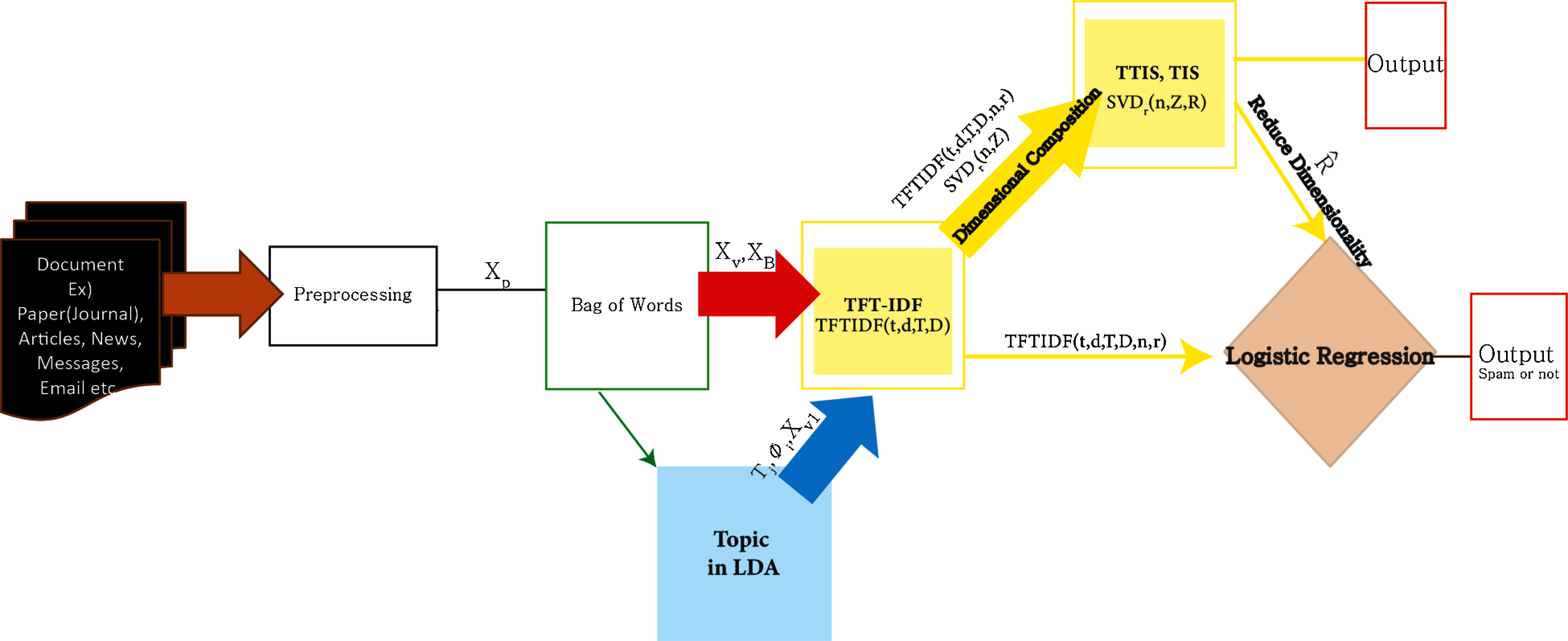
Figure 1: Structure of the overall system
The TF-IDF is equivalent to expression Eq. (4). As can be seen from the expression, the model only uses the inverse document frequency with words. However, the TFTIDF model is a weighted model that considers topic factors for spam classification in addition to word and reverse document frequencies in the document. The TFTIDF model is generated by Eq. (5).
In Fig. 1, the TFTIDF model is a module receiving red and blue arrows. Let the original data be X and preprocessed data be Xp. The data extracted from the bag-of-words (BOW) are referred to as Xb. Let Tj be the topic and Xv be the term of a dictionary. Xv1 represents a dictionary of words from LDA, where Φ is the coefficient. Then, the formula of the TFTIDF model proposed in this paper is as follows:
In the ith TFTIDF value, T stands for the topic, D stands for document, and t stands for terms. The TFTIDF value is multiplied by the frequency of the term in the ith document and the log function of the ith term of the topic in the term dictionary of the nth topic and divided by the frequency of all terms in the document. Then, it is multiplied by the calculated document weight value.
4.3 Computational Considerations
The topic is determined by the word distribution on a particular topic and the word distribution contained in the document using the Bayesian network. For these, inference-based sampling was performed using the LDA algorithm. Let us call alpha and beta potential variables. Depending on alpha and beta, the conditional probability can be represented by the following joint probability distribution [28].
Reference [28] showed that by using a generative model, knowing the distribution of topics and probability of generating a specific word for each topic, the probability of a specific document can be calculated. First, it takes N from a Poisson distribution and Theta from Dir(). A topic is selected from Multinomial(), and a word is selected based on the probability of generating words for each topic and the conditional probability of the topic.
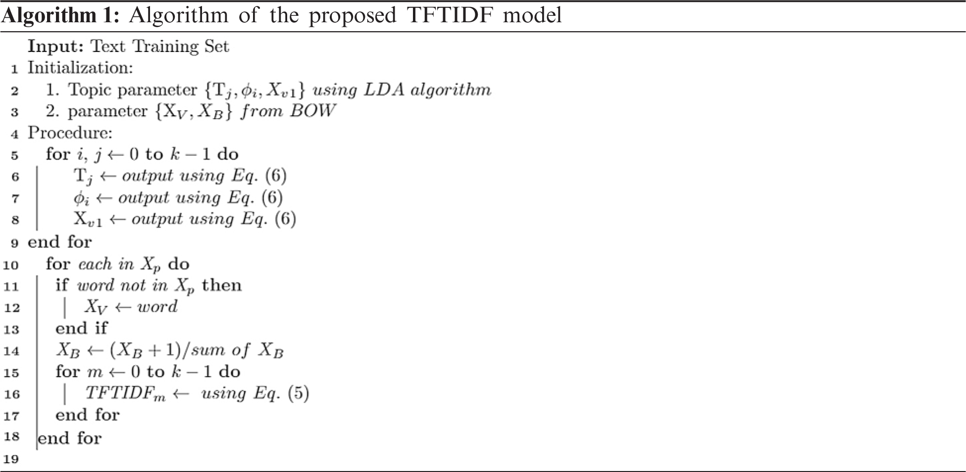
First, the formula for obtaining the i-th TFTIDF value is repeated k times.
The formula for TFTIDF (t, d, T, D, n, r) is as follows:
In the TFTIDF (t, d, T, D, n, r) model, the parameter n represents the number of term weight groups, where n = 0, 1,…, 10… r is the number of times the total matrix is decomposed, where r = 0,…, integer. Therefore, the second model proposed in this paper is as follows:
TFT-IDF in SVD consists of three logic functions. From 0 to 1, r follows the SVD (n, Zi) function, and when r is greater than 1, it follows SVD (n, Zi, R). Other values are used as classification values.
4.5 Computational Considerations
Let the original matrix be X. When the decomposition matrix is obtained, it is divided into normal orthogonal matrices U and V and Sigma matrices. Matrix XTX becomes (U∑VT)TU∑VT. That is, V∑2VT, Va is an eigenvector, and ∑a is the square root of corresponding the eigenvalue. ALS was used to determine the error of the decomposed matrix. The formula is as follows:
In addition to the factors pd and qt, this is affected by the parameters n and r and the number of ranks.
This enables faster operation and shows robustness to sparse data. We fixed the lambda value to 0.001 using L2 normalization to prevent overfitting. The Frobenius norm formula was calculated as follows:
Depending on the number of ranks, the matrices p and q were alternately updated until the error became small. The formula was calculated as this:
For this purpose, the normalized loss function L2 was used. Partial differentiation was performed to determine the optimal value to minimize the original error.
The formula was expressed in matrix form using the value calculated in the previous step,
Based on Eq. (8), it was divided into a component p when r = 1 and component p’ when r = 2, as shown in Eq. (13), and it was divided into a component q when r = 1 and a component q’ when r = 2, as shown in Eq. (14).
Eq. (13) is the sum of lambda multiplied by its own inverse matrix. This is multiplied by the inverse and is equal to qixT. Eq. (14) is the sum of lambda multiplied by its own inverse matrix. It is multiplied by the inverse procession and is equal to pixT.
Training data and testing data were divided, each value was computed, and learning was conducted.
As the result, error were found between data dimensionally decomposed with eigenvectors with large eigenvalues and the X matrix and creates a close matrix.
The following shows the algorithm of TTIS and TIS models. Parameters t refers to term, d refers to document, T refers to topic vectors, D refers to document vectors, n refers to the number of word weight group from LDA, r refers to the number of dimension decomposition where integer, Z refers to the matrix calculation between document-word and of Topic weights and R refers to decomposed matrix.
As in Eq. (8), it is calculated until the value of the error between the i-th element of the P matrix is small. For this, in order to find the optimal parameter R, Eqs. (13)–(14) are used simultaneously to alternately update and converge to Z.

The third proposed model follows the same method as the above proposed model but is decomposed using a different feature model up to r = 2. The formula is as follows:
In the third proposed model, the TF-IDF model is used, and the remaining formulae are the same as Eqs. (13)–(15).
4.7 Computational Considerations
Let the original matrix be X′. When the decomposition matrix is obtained, so are U′, V′, and Diag(D). Va′ is an eigenvector, and da′ is a high eigenvalue. ALS was used to determine the error of the decomposed matrix, as in Eq. (9), but the actual values and parameters were different.
To prevent overfitting, the lambda value was equally implemented as 0.001 using L2 normalization, and p and p′ and matrices q and q′ were alternately updated. By dividing into training and testing data-sets, each model was trained to obtain an optimal value and a classification result was produced.
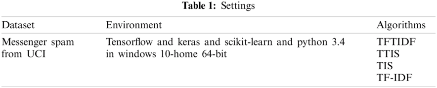
We used UCI’s messenger spam data from [29] as the dataset for the experiment. To compare the classification prediction accuracy for each model, the training and testing data were mixed at a 1:1 ratio, and an experiment was conducted for comparison and analysis. The implementation of the algorithm proposed in this paper used Tensorflow, Keras, Scikit-learn, and Python 3.4 on window 10-home 64-bit PC. The Tab. 1 shows settings.
The purpose of the experiment was to measure the classification result score, accuracy, receiver operating characteristic (ROC), similarity, and learning error for the TF-IDF, TFIDF, TF-IDF in SVD and TF-IDF in SVD, and to compare influential words. In addition, as the parameters n and r changed, the performance of the models was evaluated. Cosine similarity was used to evaluate the similarity distance, and the MSE function was used as the learning error. The results are presented in Tabs. 2 and 3.
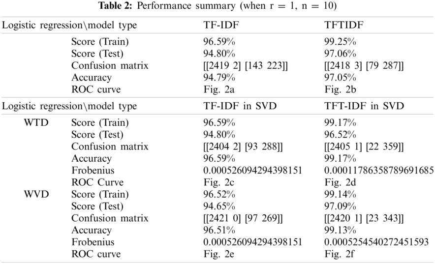
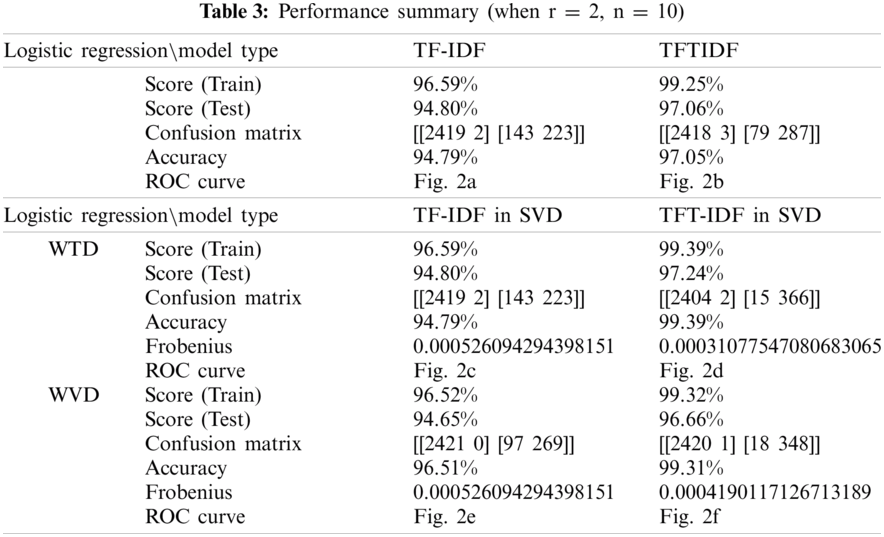
When classifying with logistic regression using the existing TF and IDF features, the classification score calculated during training with train data was 96.59%. After testing with the remaining 50% of the data, the classification score was 94.80%. To obtain a better classification performance, we measured the accuracy of the confusion matrix. The existing TF-IDF model classified spam correctly with 94.79% accuracy. The ROC curve of this model is shown in Fig. 2a. The ROC value consisted of tpr was 0.98.
When classifying using TFTIDF, the classification score calculated during training with Train data was 99.25%. After testing with the remaining 50% of the data, the classification score was 97.60%. To obtain a better classification performance, we measured the accuracy of the confusion matrix. When classifying using the TFTIDF model proposed in this paper, spam was classified correctly with an accuracy of 97.05%. The ROC curve of this model is shown in Fig. 2b. The ROC value was 0.98.

Figure 2: ROC curves. From the top left [r = 1, (a) TF-IDF, (b) TFTIDF, (c) When Train data, TF-IDF in SVD, (d) When Train data, TFT-IDF in SVD, (e) When validation data, TF-IDF in SVD, (f) When validation data, TFT-IDF in SVD]. [r = 2, (a) TF-IDF, (b) TFTIDF, (c) When Train data, TF-IDF in SVD, (d) When Train data, TFT-IDF in SVD, (e) When validation data, TF-IDF in SVD, (f) When validation data, TFT-IDF in SVD]
Specifically, when comparing the classification results using the training data of the two models, the TFTIDF model performed approximately 2.66% better than the TF-IDF model. Moreover, the results of the classification performance experiment using the testing data showed that the TFITIDF model scored 2.26% higher than the existing TF-IDF model. Therefore, it can be seen that binary classification using the TFTIDF model is more effective than that using the existing TF-IDF model.
When classifying with logistic regression using features of the existing TF-IDF, the classification score calculated during training with Train data was 96.59%. After testing the remaining 50% of the data, the classification score was 94.80%. The TF-IDF model classified spam with an accuracy of 94.79%. The ROC value was 0.98. When classifying using TFT-IDF in SVD, the classification score for training was 99.17%. After testing with the remaining 50% of the data, the classification score was 96.52%.
Moreover, the training score calculated during training with validation data was 96.52%, and the testing data classification score was 94.65%. When learning with validation data, the calculated training classification score was 99.14%, and the test score was 97.09%. We learned using the MSE function. When the TFT-IDF in SVD model was trained and classified, the classification was predicted with an accuracy of approximately 99.17%. When classification was performed using validation data and the TFT-IDF in the SVD model, the prediction accuracy was 99.13%. The ROC curves of this model are shown in Figs. 2d and 2f. The calculation of the Frobenius norm yielded results of approximately 0.000117863 and 0.000525454027 for training and testing, respectively. The corresponding matrices are shown in Tab. 2, respectively. The ROC value of this model was 0.98.
Specifically, when comparing the classification results of the TF-IDF and TFT-IDF in SVD models using the training data and testing data, the accuracy of the latter was higher than that of the former by (train) 4.38% and (test) 4.35%. As a result, it was found that the binary classification using the TFT-IDF in the SVD model proposed in this paper has a more effective performance than binary classification using the existing TF-IDF model.
Conducting classification using the TF-IDF in SVD model projected by reducing the dimensions of the features of the existing word frequency and IDF when learning with training data, the calculated classification score was 96.59%. After testing the remaining 50% of the data, the classification score was 94.80%. Moreover, the score calculated during training the validation data was 96.52%, and the test score was 94.65%. All models were trained using the MSE function as an error function during training. Classification using the training data and the TF-IDF in the SVD model, the classification accuracy was approximately 96.59%. When classification was performed using validation data and the TF-IDF in the SVD model, the prediction accuracy was 96.51%. The ROC curves of the model are shown in Figs. 2c and 2e. The Frobenius norm calculations resulted in all values being approximately 0.0005260942. The corresponding matrices are shown in Tab. 2. The values of the ROC of this model were 0.98 and 0.9 for training and testing, respectively.
There was no difference between the two models when using Train TF-IDF in SVD, which compared the classification results of the two models TF-IDF and TF-IDF in SVD for the training and testing data. On the other hand, when using the validation TF-IDF in SVD, the train score was approximately 0.07% lower, and the test score was approximately 0.15% lower than that using the existing TF-IDF model.
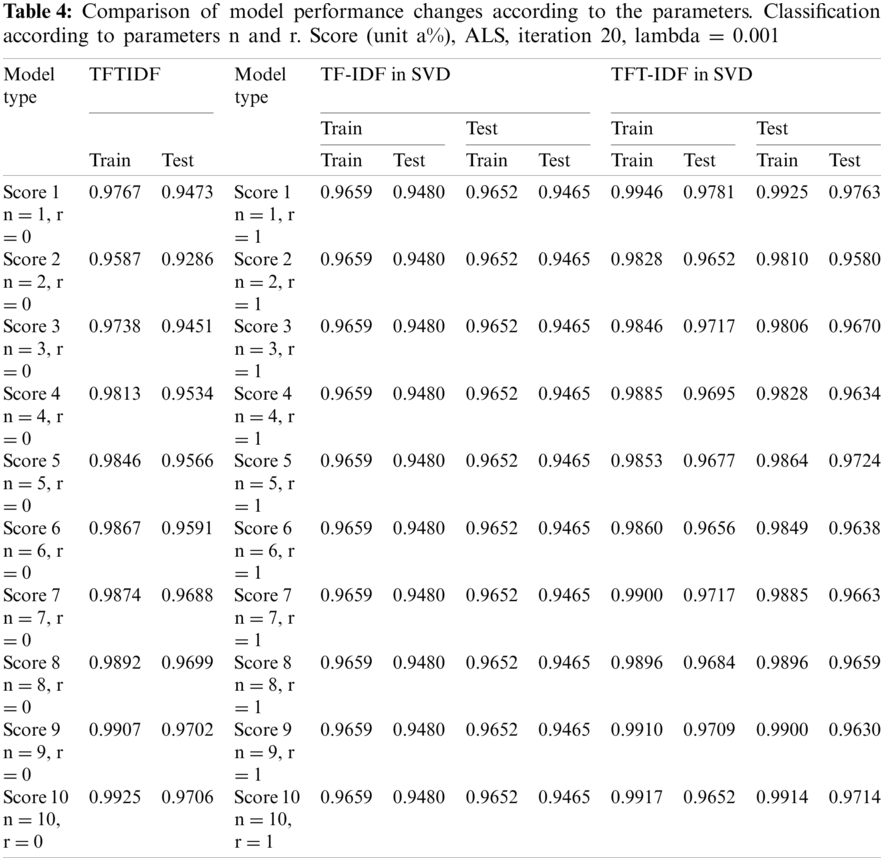
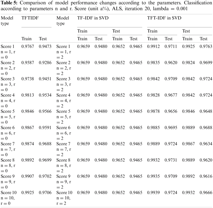
5.6 Comparison of Model Performance Changes According to the Parameters
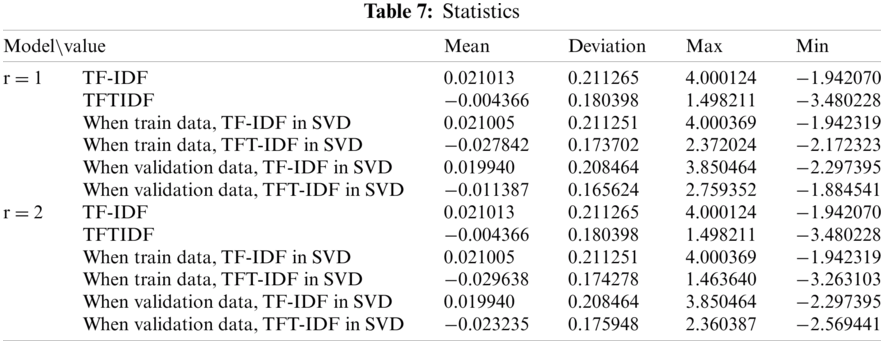
As the parameters of the proposed models change, performance evaluation was conducted. ‘r’ is the number of times the total matrix is decomposed. The experiment was performed by disassembling only up to the first and second total. ‘n’ is a parameter that affects the weight between documents and topics and between topics and words, representing the number of word weight groups. The results are shown in Tabs. 4 and 5. The TF-IDF model shows that the training and the testing scores are constant at 0.9659 and 0.9480, respectively, regardless of parameter n. In the TFTIDF model, it can be seen that the training score decreases as n increases from 1 to 2, and then continues to increase from n = 3 onwards. ‘n’ made the most noticeable change between 1 and 2 (0.018). The test score value of the TFTIDF model also decreased at n = 1 and n = 2 and continued to increase from n = 3. ‘n’ achieved the most significant increase/decrease between 1 and 2 (0.0187). In the training model of the TF-IDF in the SVD model, when n = 1 and r = 1, the training and testing values were 0.9659 and 0.9480, respectively, and all were the same without any change in values. In the training of the TFT-IDF in the SVD model, the highest score was approximately 0.9946 when n = 1 and r = 1. As n increased, it decreased and then increased again. Finally, it converged to 0.9917 for n = 10. In the training of TFT-IDF in SVD, the testing score was also highest when n = 1 and r = 1, and gradually decreased and then increased repeatedly, forming a jagged pattern. In the training of TFT-IDF in SVD, the highest score also occurred when n = 1 and r = 1, and the change took a convex form that gradually decreased and then increased. It was confirmed that the logistic classification results were affected by the parameters ‘n’ and ‘r’ and the L2 error function of SVD. The results of measurement and the statistics of the models are shown in Tabs. 6 and 7, respectively.
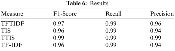
This paper proposed the TFIDF and TFT-IDF in the SVD models, which improved the TF-IDF model and TF-IDF in the SVD models. We evaluated the results using a binomial classification model. Calculating the score, accuracy, and ROC results of the classified experiment, the TFTIDF model at n = 10 showed an approximately 2.26% higher score than the existing TF-IDF feature model. The TFT-IDF in the SVD model, was trained and classified spam. It achieved a prediction accuracy of approximately 99.17% when r = 1, n = 10, outperforming the TF-IDF model. In addition, the model with r = 2, n = 10 showed the highest performance among the models, with an accuracy of 99.39%. However, the TF-IDF in the SVD model showed an approximately 0.07% lower training score and 0.15% lower testing score than binary classification using the existing TF-IDF model. Overall, document predictability was significantly improved compared to using only TF-IDF. In addition, the TFT-IDF in the SVD model presents a reasonable solution to the scarcity problem encountered in the existing TF-IDF model and effectively reduced the dimension to achieve superior performance. It is expected to improve theoretical and practical value by applying genuine bot services and theoretical research for many ML algorithms.
Acknowledgement: This work was supported by the BK21 FOUR Project etc.
Funding Statement: This work was supported by the BK21 FOUR Project. W.H.P received the grant. (https://www.bk21four.nrf.re.kr).
Conflicts of Interest: The authors declare that they have no conflicts of interest to report regarding the present study.
1. W. K. Lee, “A study on spam mail regulation policy in cyberspace,” Regulatory Study, vol. 13, no. 2, pp. 201–227, 2004. [Google Scholar]
2. J. Wan, “Spam mail flooding and regulatory measures,” Criminal Policy Research Institute, vol. 77, pp. 1–48, 2003. [Google Scholar]
3. H. W. Lee and H. C. Ahn, “Optimization of classification criteria considering asymmetric error costs and an intelligent intrusion detection model based on SVMs,” Intelligent Information Research, vol. 17, no. 4, pp. 157–173, 2011. [Google Scholar]
4. M. Alauthman, “Botnet spam e-mail detection using deep recurrent neural network,” International Journal of Emerging Trends in Engineering Research, vol. 8, no. 5, pp. 1979–1986, 2020. [Google Scholar]
5. G. J. Luo, N. Shah, U. K. Habib and U. H. Amin, “Spam detection approach for secure mobile message communication using machine learning algorithms,” Security and Communication Networks, vol. 2020, pp. 1–6, 2020. [Google Scholar]
6. A. Najeeb and N. Fuhr, “Language models, smoothing, and IDF weighting,” in Proc. LWA, Kassel, Germany, pp. 169–174, 2010. [Google Scholar]
7. S. M. Mustafa and A. Yasar, “Performance analysis of ANN and naive bayes classification algorithm for data classification,” International Journal of Intelligent Systems and Applications in Engineering, vol. 7, no. 2, pp. 88–91, 2019. [Google Scholar]
8. G. Zou, “A modified poisson regression approach to prospective studies with binary data,” American Journal of Epidemiology, vol. 159, no. 7, pp. 702–706, 2004. [Google Scholar]
9. P. Peter, C. John, K. Elizabeth, R. H. Theodore and R. F. Alvan, “A simulation study of the number of events per variable in logistic regression analysis,” Journal of Clinical Epidemiology, vol. 49, no. 12, pp. 1373–1379, 1996. [Google Scholar]
10. R. E. Fan, K. W. Chang, C. J. Hsieh, X. R. Wang and C. J. Lin, “LIBLINEAR: A library for large linear classification,” The Journal of Machine Learning Research, vol. 9, pp. 1871–1874, 2008. [Google Scholar]
11. J. H. Friedmann, T. Hastie and R. Tibshirani, “Additive logistic regression: A statistical view of boosting,” The Annals of Statistics, vol. 28, no. 2, pp. 337–407, 2000. [Google Scholar]
12. W. Taylor, G. Dafna, H. Philip, M. Antonio, M. Philip et al., “Classification criteria for psoriatic arthritis: Development of new criteria from a large international study,” Arthritis & Rheumatism: Official Journal of the American College of Rheumatology, vol. 54, no. 8, pp. 2665–2673, 2006. [Google Scholar]
13. D. R. Cutler, C. E. Thomas, H. B. Karen, C. Adele, T. H. Kyle et al., “Random forests for classification in ecology,” Ecological Society of America, vol. 88, no. 11, pp. 2783–2792, 2007. [Google Scholar]
14. O. Aytuğ, S. Korukoğlu and H. Bulut, “Ensemble of keyword extraction methods and classifiers in text classification,” Expert Systems with Applications, vol. 57, no. 15, pp. 232–247, 2016. [Google Scholar]
15. O. Aytuğ, S. Korukoğlu and H. Bulut, “A multiobjective weighted voting ensemble classifier based on differential evolution algorithm for text sentiment classification,” Expert Systems with Applications, vol. 62, no. 15, pp. 1–16, 2016. [Google Scholar]
16. J. Zhao and G. Xiaolin, “Comparison research on text pre-processing methods on twitter sentiment analysis,” IEEE Access, vol. 5, pp. 2870–2879, 2017. [Google Scholar]
17. M. R. Aassih and C. Goutte, “A co-classification approach to learning from multilingual corpora,” Machine Learning, vol. 79, no. 1, pp. 105–121, 2010. [Google Scholar]
18. P. Tomas and V. Marcinkevičius, “Comparison of naive bayes, random forest, decision tree, support vector machines, and logistic regression classifiers for text reviews classification,” Baltic Journal of Modern Computing, vol. 5, no. 2, pp. 221–232, 2017. [Google Scholar]
19. C. Andres, P. Denis, L. Hans and S. Alvaro, “Automatic document screening of medical literature using word and text embeddings in an active learning setting,” Scientometrics, vol. 125, no. 3, pp. 3047–3084, 2020. [Google Scholar]
20. M. A. Mohammed, A. I. Dheyaa, O. S. Akbal, A. M. Salama, M. Aida et al., “Adaptive intelligent learning approach based on visual anti-spam email model for multi-natural language,” Journal of Intelligent Systems, vol. 30, no. 1, pp. 774–792, 2021. [Google Scholar]
21. M. A. Mohammed, S. G. Saraswathy, A. M. Salama, M. Aida and K. A. G. Modh, “Implementing an agent-based multi-natural language anti-spam model,” in Int. Symp. on Agent, Multi-Agent Systems and Robotics, Putrajaya, Malaysia, IEEE, pp. 1–5, 2018. [Google Scholar]
22. D. W. Hosmer, T. Hosmer, S. L. Cessie and S. Lemesohw, “A comparison of goodness-of-fit tests for the logistic regression model,” Statistics in Medicine, vol. 16, no. 9, pp. 965–980, 1997. [Google Scholar]
23. G. Alexander, D. L. Lewis and M. David, “Large-scale bayesian logistic regression for text categorization,” Technometrics, vol. 49, no. 3, pp. 291–304, 2007. [Google Scholar]
24. B. J. Lee and Y. G. Jung, “Features reduction using logistic regression for spam filtering,” The Journal of the Institue of Internet, Broadcasting and Communication, vol. 10, no. 2, pp. 13–18, 2010. [Google Scholar]
25. X. Tian and T. Wang, “An improvement to TF: Term distribution based term weight algorithm,” in Second Int. Conf. on Networks Security, Wireless Communications and Trusted Computing, Wuhan, China, vol. 1, pp. 252–255, 2010. [Google Scholar]
26. J. Ramos, “Using TF-IDF to determine word relevance in document queries,” in Proc. The first Instructional Conf. on Machine Learning, Angeles, Philippines, vol. 242, no. 1, pp. 29–48, 2003. [Google Scholar]
27. Y. Hua and J. Yang, “A direct LDA algorithm for high-dimensional data—with application to face recognition,” The Journal of the Pattern Recognition Society, vol. 34, no. 10, pp. 2067–2070, 2001. [Google Scholar]
28. B. David, M. Andrew, Y. Ng and M. I. Jordan, “Latent dirichlet allocation,” The Journal of machine Learning Research, vol. 3, pp. 993–1022, 2003. [Google Scholar]
29. M. G. H. José, A. A. Tiago and Y. Akebo, “On the validity of a new SMS spam collection,” in 11th Int. Conf. on Machine Learning and Applications, Boca Raton, FL, USA, vol. 2, pp. 240–245, 2012. [Google Scholar]
 | This work is licensed under a Creative Commons Attribution 4.0 International License, which permits unrestricted use, distribution, and reproduction in any medium, provided the original work is properly cited. |