DOI:10.32604/cmc.2022.019636
| Computers, Materials & Continua DOI:10.32604/cmc.2022.019636 | |
| Article |
Malicious Traffic Detection in IoT and Local Networks Using Stacked Ensemble Classifier
1School of Computing and Mathematics, Charles Sturt University, Australia
2Department of Computer Science, Broward College, Broward County, Florida, USA
3School of Computing and Information Sciences, Florida International University, USA
4Department of Computer Science, Khwaja Fareed University of Engineering and Information Technology, Rahim Yar Khan, Pakistan
5Department of Information and Communication Engineering, Yeungnam University, Gyeongsan-si, 38541, Korea
*Corresponding Author: Imran Ashraf. Email: ashrafimran@live.com
Received: 20 April 2021; Accepted: 03 June 2021
Abstract: Malicious traffic detection over the internet is one of the challenging areas for researchers to protect network infrastructures from any malicious activity. Several shortcomings of a network system can be leveraged by an attacker to get unauthorized access through malicious traffic. Safeguard from such attacks requires an efficient automatic system that can detect malicious traffic timely and avoid system damage. Currently, many automated systems can detect malicious activity, however, the efficacy and accuracy need further improvement to detect malicious traffic from multi-domain systems. The present study focuses on the detection of malicious traffic with high accuracy using machine learning techniques. The proposed approach used two datasets UNSW-NB15 and IoTID20 which contain the data for IoT-based traffic and local network traffic, respectively. Both datasets were combined to increase the capability of the proposed approach in detecting malicious traffic from local and IoT networks, with high accuracy. Horizontally merging both datasets requires an equal number of features which was achieved by reducing feature count to 30 for each dataset by leveraging principal component analysis (PCA). The proposed model incorporates stacked ensemble model extra boosting forest (EBF) which is a combination of tree-based models such as extra tree classifier, gradient boosting classifier, and random forest using a stacked ensemble approach. Empirical results show that EBF performed significantly better and achieved the highest accuracy score of 0.985 and 0.984 on the multi-domain dataset for two and four classes, respectively.
Keywords: Stacked ensemble; PCA; malicious traffic detection; classification; machine learning
Internet services are widely utilized by businesses, industries, education, and in a variety of other fields of human life. In the past two decades, the advent of information technology made network infrastructure essential for individuals, as well as, corporate organizations [1]. In addition to an exponential growth in reliance on internet services for network infrastructures, the integrity, confidentiality, security, and availability of sensitive information have been compromised increasingly due to various kinds of malicious attacks. Individuals and corporate organizations are impelled to integrate safety mechanisms such as antivirus software, firewall, or malware detection system in their network to secure critical data from such malicious attacks. Depending only on the conventional firewall is inadequate for business networks as the prevention of different forms of malicious attacks cannot be achieved [2]. The particular reason for this circumstance is that malicious attacks have become more complicated and diversified over the past few years making a conventional firewall ineffective for modern attacks. Hence, in addition to a firewall, a malicious traffic detection system (MTDS) is integrated into the network infrastructure to enhance the security and ensure the credibility of the system [3]. An MTDS acts as a wall of defense for a network infrastructure against malicious attacks. MTDS attempts to detect the deviation of network traffic from traditional patterns of traffic usage and flags it as malicious traffic or intrusion and authorizes only non-malicious traffic to the end-users.
Detection of malicious traffic in a network system can be categorized as network-based and host-based malware detection [4]. A host-based malicious traffic detection system (HMTDS) assesses network data at the host level while the network-based malicious traffic detection system (NMTDS) analyzes online network traffic data of any malware at the server or network gateway before the malware reaches the end-user. Additionally, NMTDS can function online as well as offline. An offline NMTDS logs network information to detect any intrusion while an online NMTDS inspects network traffic for detection of malicious activity as it arrives [5].
This study focuses on real-time NMTDS where the incoming traffic is captured and analyzed for any suspected malware. The detection of malware results in blocking the traffic to secure the end-user from ongoing attacks. The proposed framework can also be integrated with HMTDS along with the categorization of network traffic as local network traffic and IoT network traffic. A general framework of the proposed MTDS is shown in Fig. 1. The proposed MTDS is designed using machine learning algorithms for the detection of malicious traffic from local network traffic as well as IoT network traffic. For this purpose, two publicly available datasets; UNSW-NB15 and IoTID20 are utilized. The implementation of machine learning algorithms provides us with a straightforward and systematic approach for malicious traffic detection which provides easy adaptation and control. To achieve this, we integrated and compared several machine learning algorithms including random forest (RF), logistic regression (LR), gradient boosting classifier (GBC), decision tree classifier (DTC), extra tree classifier (ETC), stochastic gradient descent classifier (SGDC), and k-nearest neighbor (KNN) for classifying network traffic as an anomaly (1) and normal (0).
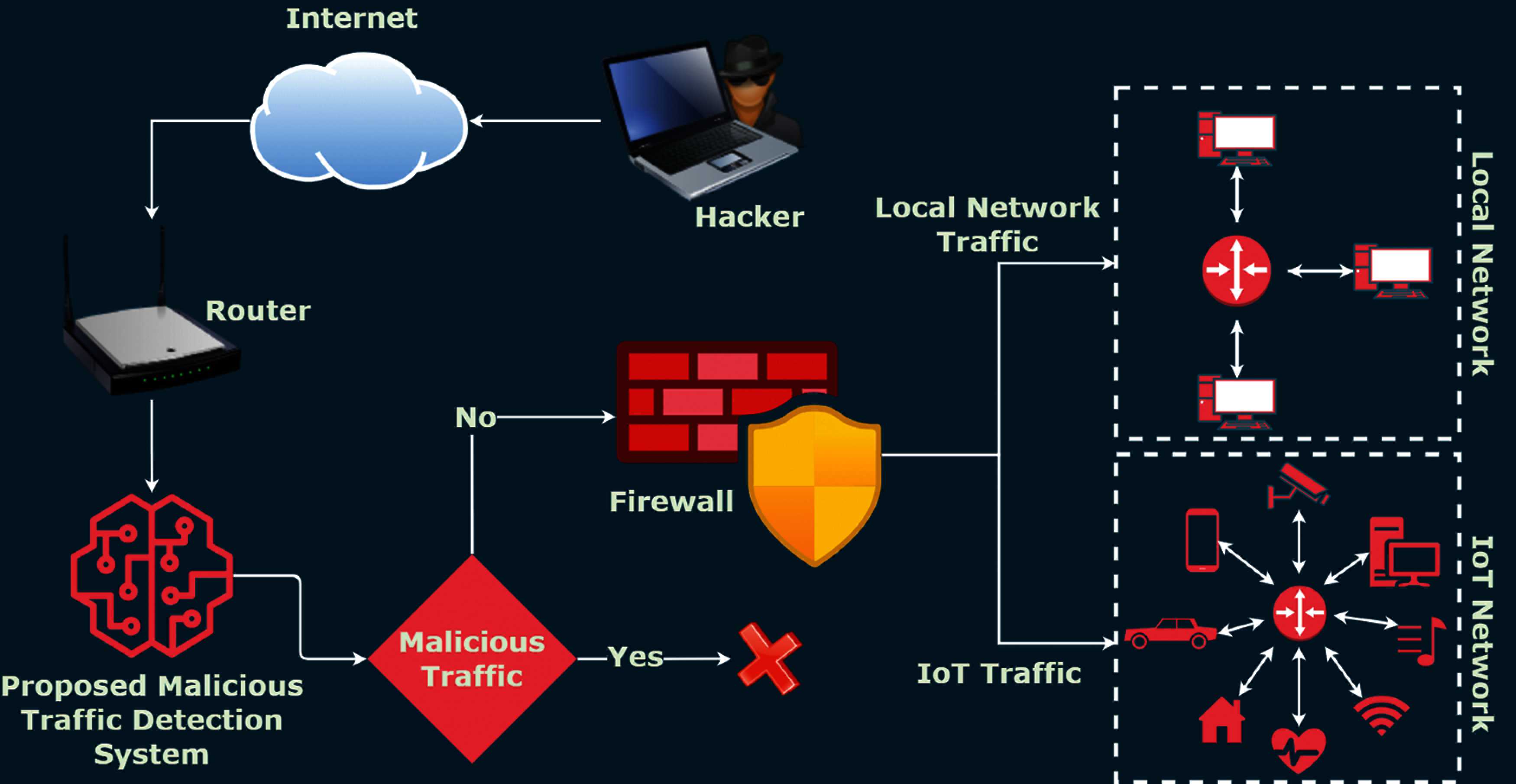
Figure 1: General framework of the proposed malicious traffic detection system
Even though there are a variety of features that could be leveraged for MTDS, we integrated principal component analysis (PCA) to consider only 30 features from each dataset. The proposed MTDS is evaluated both for binary classification and multi-classification to provide extensive analysis of the approach and increase its credibility. The current study is proposed for the detection of malicious traffic from IoT and local network traffic by using PCA as a dimensionality reduction technique and to enhance the performance of machine learning models. However, fundamental contributions in this study are summarized below.
• This study proposes a novel approach to monitor and detect malicious traffic in an IoT and local network infrastructure. The stack ensemble approach, called extra boosting forest (EBF) aims at detecting malicious traffic using tree-based models as base-learners. The primary objective is on real-time NMTDS to monitoring the incoming traffic and analyzing for suspected malware.
• The proposed approach is tested on a complex dataset by combining features of the IoT network traffic dataset (IoTID20) and local network traffic dataset (UNSW-NB15). Horizontal merging of the datasets is achieved by obtaining an equal number of features from both the datasets through the PCA approach.
• The proposed approach is evaluated with binary classification as well as multi-class classification in terms of accuracy, precision, recall, and f1-score. Additionally, comparative performance analysis is conducted using various machine learning classifiers, as well as, state-of-the-art approaches.
The rest of the paper is divided into five sections: Section 2 provides the literature review while Section 3 contains the description of the proposed approach and the datasets used for training and testing. Results and discussion are provided in Section 4 while the concluding remakes are given in Section 5.
Despite Malware is a fast-growing threat to the security of information and sensitive data in computer systems. Malware exploits the vulnerabilities of a system or network infrastructure and the detection of malware has been regarded as a significant research area. Several techniques have been developed by the researchers to identify malware by integrating many machine learning (ML), as well as, deep learning (DL) techniques.
Malware changes the data structures of programs leaving its fingerprints on memory accesses of the program. Based on these patterns of changes in data structures, a study [6] identified the behavior of malicious attacks on application-specific virtual memory access patterns of the kernel as well as a user-level rootkit. In this study, 10% of the features with the highest F-score were selected. The study utilized RF and LR classifiers to achieve 100% accuracy in the detection of malicious attacks of the kernel-level rootkit. While for the user-level rootkit, malicious attacks were identified with an accuracy of 99% by RF. In the same way, another study [7] proposed a method for the automated classification of malware. The approach has the capability of detecting new forms of malware. The study utilizes the data collected from Threat Trace Security from the campus network, VX Heavens and ESET NOD32. Several features have been used in this study including import functions, Opcode n-gram, and grey-scale images with the integration of an enhanced information gain for the dimensional reduction of extracted features. The study utilized DT, support vector machine-poly (SP), LR, Naïve Bayes (NB), gradient boosting (GB), KNN, and RF for the classification of malware and shared nearest neighbor (SNN) for detection of new malware. The proposed system achieved the highest accuracy of 98.9% with RF for the classification of unknown malware and detects new malware with an accuracy of 86.7%.
Along the same direction, the authors performed malware detection on malware samples acquired from the Malicia project and benign samples extracted from several windows systems [8]. The study utilized opcode frequency for the extraction of features and then further reduced the dimensionality of feature vector space by making use of none, variance threshold (VT), and single and a three-layered auto-encoder (AE-1L and AE-3L), respectively. For classification purposes, the study incorporated RF, a deep neural network (DNN) with two, four, and seven layers (DNN-2L, DNN-4L, and DNN-7L), respectively. Experimental results showed that RF with VT outperformed DNNs with an accuracy of 99.78%. One of the significant reasons for the drastic increase in malicious attacks is developers’ exploitation of malware where minor changes in the already available malware lead to introducing a new malware in the network. So, detection of such variations is of significant importance for the security of sensitive data. In this regard, an approach based on deep learning to detect malware in Microsoft and Malimg datasets was proposed in [9]. The study converts the features extracted from the datasets into greyscale images since a minor change in the code of the malware is easy to track in an image. The study utilizes the convolutional neural networks (CNN) for classification and achieved 99.97% and 98.52% accuracy on Microsoft and Malimg datasets, respectively.
A malware classification system called ‘Malscore’ was proposed in [10] which is based on machine learning models and probability scoring. The proposed system works in two phases, where, CNN is utilized with spatial pyramid pooling to examine grayscale images in phase 1, and several n-grams and ML models have been integrated to examine the dynamic features in phase 2. The study utilized 63 malware families and collected 174,607 malware samples. For phase 2, the features were extracted by making use of n-grams of lengths 2, 3, and 4. The selection of features was carried out by document frequency-inverse document frequency (DF-IDF) approach. The study trained five machine learning models including RF, SVM, NB, AdaBoost, and KNN. Evaluation of Malscore showed that it classified malware with an accuracy of 98.82%. Another study [11] advanced the process of malware detection by integrating effective and low-dimensional features with an ensemble of tree-based methods. The study showed that tree-based ensemble methods perform better with low-dimensional features which do not require padding or selection of fixed length features. Consequently, word2vec, a feature extraction method for deep learning models was utilized by [12] for the vector representation of malware based on the opcode. The study utilized the GB algorithm to validate the system using k-fold cross-validation and achieved an accuracy of 96%.
Application programming interface (API) functions along with opcodes are utilized in another study [13] for the classification of malware by integrating a word2vec based long short-term memory (LSTM). The study carried out experiments on the Microsoft dataset and acquired an accuracy of 97.59%. Similarly, several frameworks were proposed in [14] that used language models based on the gated-recurrent unit (GRU), LSTM, and character-level convolutional neural network (CCNN). The study showed that features extracted by LSTM lead to improved accuracy in comparison to the architectures integrating random-weighted features. Similarly, feature selection techniques including chi-square, gain ratio, information gain, and fisher score are utilized for the classification of malware from Microsoft dataset by the authors in [15]. The study took advantage of machine learning classifiers including simple cart (SC), random tree (RT), J48 Graft, Naïve Bayes tree (NBT), REPTREE, J48, RF, logistic model tree (LMT), and decision stump (DS). The study concluded that the fisher score outperformed other feature selection techniques for RF, NBT, LMT, and RT with an accuracy of 100%.
Classification performance of malware detection is highly influenced by the features which are used for models ‘training. As a result, several research works investigate the importance of various feature selection methods to increase the efficacy of malware detection. The authors perform an analysis of various feature selection techniques including L1-regularized methods, Chi-square, F-statistics, and Relief F in [16]. The study concluded that the L1-regularized embedded feature selection technique produces more correlated features for the models to perform classification tasks. The authors of the study [17] eliminated the implementation of domain knowledge for the extraction of required features and automated the feature section process by integrating opcodes up to 10-grams. The study experimented on 2520 samples and resulted in a 98% f-measure. Another study [18] integrated machine learning and deep learning approaches for malware classification by integrating an RF model combined with opcodes, VT, AE-1L, and AE-3L, and DNN with two, four, and seven layers combined with auto-encoders. The experimental results of the study showed that RF with VT achieved the highest accuracy of 99.78% while DNN with AE-1L gave an accuracy of 99.21%. Results suggest that the machine learning models outperformed deep learning models for malware detection. The findings of the above-discussed research works are summarized in Tab. 1. Despite the reported accuracy, several aspects of malware detection approaches are not explored extensively. For example, the differentiability of the selected features for malware detection is not studied very well. Similarly, the robustness of malware detection approaches is not elaborated for online network traffic which is very important. The threats from multi-domain malware are not investigated either. So, this study focuses on malware detection from multi-domain network traffic with increased accuracy.

This section contains a description of the datasets used for the experiments, as well as, the details of the proposed approach to detect the malicious traffic.
The proposed system is evaluated by using two publicly available datasets including the UNSW-NB15 dataset https://www.unsw.adfa.edu.au/unsw-canberra-cyber/cybersecurity/ADFA-NB15-Datasets/ [19] and IoTID20 https://ieee-dataport.org/open-access/iot-network-intrusion-dataset. Despite the UNSW-NB15 being the old dataset, it contains patterns of recent attacks and is still one of the widely used benchmark datasets publicly available for evaluation of malware detection systems. Whereas, IoTID20 is the contemporary dataset collected by authors of [20] in an IoT environment which is an up-to-date dataset consisting of real-time traffic of recent attacks. Therefore, to compare our proposed approach with state-of-the-art malware detection techniques we adopted a hybrid of the UNSW-NB15 dataset and a latest IoTID20 dataset. The datasets are combined for a variety of purposes. For example, since each dataset has a different number of samples for each class which creates the data imbalance problem, combining the datasets resolves this problem. Similarly, the UNSW-NB15 dataset contains the data for local traffic while IoTID20 contains real-time IoT traffic data. Machine learning algorithms tend to show good performance on individual datasets. However, to evaluate the performance of the proposed approach, both datasets are combined to make a complex dataset that contains both local and real-time traffic.
The datasets are combined because these datasets efficiently resolve the issue of data imbalance between legitimate and illegitimate connection records.
The UNSW-NB15 dataset has around 100 GB volume of network packets producing 2,540,044 connection records of which 321,283 are illegitimate and 2,218,761 are legitimate. The UNSE-NB15 is a high-dimensional dataset containing 47 attributes for each connection record. The attribute ‘label’ has a binary value of 0 and 1 which corresponds to ‘normal and ‘anomaly, respectively. The velocity of this dataset is 5–10 MBs on average which portrays the real-world environments as shown in Tab. 2.
IoTID20 dataset was generated by implementing an IoT environment consisting of two devices including EZVIZ Wi-Fi camera and SKTNGU, a smart home device that was connected to a Wi-Fi router thus duplicating modern trends. The authors used CICflowmeter for extraction of features from Pcap files and generated CSV files of the dataset consisting of 625,783 records among which 40,073 belong to the normal class whereas, 585,710 are labeled as anomaly connection records. Each connection record has 80 attributes making it a high dimensional dataset as shown in Tab. 3. The number of samples in each dataset is shown in Tab. 4.


We perform feature reduction on both datasets using the PCA approach. PCA is a statistical algorithm that creates a feature subspace by transforming a set of highly correlated attributes into a set of attributes that are linearly uncorrelated to reduce the dimensionality of the dataset [21]. It accomplishes dimensionality reduction by identifying the direction of maximal variations which are also known as principal components (PCn) [22]. The PCn is acquired by breaking the original data into eigenvalues (a number corresponding to the amount of variance in the data) and eigenvectors (the direction where most of the variance lies in the data) [23]. Generally, PCA works by corresponding original data attributes into a new coordinated system in which PC1 (first-principal-component) is projected in the direction where data varies the most, thus capturing most of the variation in the dataset [24]. Then, PC2 is projected along the direction where data varies the most after PC1, thus, capturing the variation which was not captured by PC1. Each PCn captures most of the variation which has not been captured by the subsequent PCn–1 till the decomposition of the data matrix. The total number of dimensions of the new feature set created by PCA is equal to the total number of PCn that have been created in the process. Most significantly, the last PCn captures the least variance and hence can be omitted resulting in lower dimensionality of the dataset [25].
Let the dataset be an m×n matrix ‘Y’, where each row of Y, the vector yi represents a single record of all attributes and each column Yj represents all the records relating to one attribute of the dataset. Set of inputs Y1,Y2,Y3,…,YN are transformed linearly into another set of input columns C1,C2,C3,…,CN by PCA to overcome collinearity and high-dimensionality. Here, the first few Cs capture the most amount of variation in input data matrix Y, thus providing low dimension and minimum loss of information by eliminating the few of the last Cs. This linear transformation is carried out by an n×n matrix ‘C’ giving transformed variables C as C=YP, which alternatively decomposes Y as Y=CPC. Where P is a loading matrix YC Y of eigenvectors of highly associated eigenvalues. Thus, PC1 is calculated by subtracting c1p'1 from Y where c1 is the score of first PC and p'1 is the first loading matrix from the sample matrix Y. This gives a residual value R1 where R1 = Y − c1p'1 which further becomes Y while calculating PC2. This process is repeated until the required number of PCn is achieved. The nth principal component PCn is calculated by following the steps described below:
Step 1: Vector yj = cn:cn is taken from Y
Step 2: Pn:Pn is calculated as P′n: P′n=c′n Y/c′n cn
Step 3: Length of P′n is normalized as: 1:p′nnew=P′nold/(P′nold)
Step 4: cn:cn is calculated as: cn:cn=Ypan/P′nPn
Step 5: Difference between cn used in the second step and fourth step is observed
If there lies a difference between them then these steps are iterated, else if they give us the last PC. After the generation of PC1, Y in the second and fourth steps are replaced by the residual value R. Thus, the nth PC gives us the intrinsic dimension as employed by authors of [26] for the prediction of loss path. PCA aims at the selection of potentially significant features among all feature components of the dataset [27] which in turn improves the accuracy of machine learning models as stated by authors of [28] in which they carried out the detection of narcotics from Raman spectra by integrating PCA for feature detection and machine learning models for classification.
3.3 Supervised Machine Learning Models
In this study, we used supervised machine learning models for the detection of attacks in network traffic. The used models are tuned with the best hyperparameter settings using hit and trial methods. All hyperparameters for the learning models are shown in Tab. 5.

RF is a tree-based ensemble model that can be used both for classification and regression [29]. RF fits the number of decision trees in the learning procedure and then combines their predictions using majority voting criteria where the predicated class is based on the predictions of the higher number of decision trees [30]. RF uses the Gini value and Entropy algorithms to build the decision tree. These algorithms find the important features to build the tree and the top node will be the most important feature. Mathematically, RF can be defined as:
where
Here
RF is trained with three hyperparameters including are max_depth, n_estimators, the criterion which are shown in Tab. 5. The max_depth hyperparameter is used with the value 300 which means each decision tree in RF will be restricted to 300 level depth.
3.3.2 Decision Tree Classifier
DTC is a combination of mathematical techniques which integrates generalization, categorization, and description of a given training data into rules or tree [31]. After derivation of rules or trees in the learning phase, test data is randomly taken from the training set to test the accuracy of a decision tree. Afterward, the decision tree model is validated by utilizing unannotated data by using rules or trees derived in the learning phase of the model. The framework of a decision tree consists of a root node, a right subtree, a left subtree, and a leaf node. Each node nt in a decision tree is selected based on the highest value of selection function S(ni) which is of the form:
where
Tab. 5 shows the hyperparameters integrated for the training of DTC in the current study. DTC is subjected to max_depth = 30 which corresponds to the depth of each decision tree to 30. The selection hyperparameter i.e., criterion = entropy which represents that each node split in the decision tree will be dependent on the highest entropy score yielded by the node.
TC is an ensemble of a large number of decision trees (DT) where each DT is grown by integrating the whole training set. The framework of ETC resembles DT and initializes with a root node [32]. At every child node, ETC integrates a set of m randomly selected features i.e., Fi where
Here
3.3.4 Stochastic Gradient Descent
Gradient descent is a convex function-based optimization method that smooths a set of attributes by integrating partial differential equations or PDEs through several iterations [34]. GD minimizes the cost function C(P) by updating a set of parameters (P) to achieve a local minimum. GD integrates learning rate L for the whole training set, which defines the number of steps that are required to yield a local minimum. Incorporation of the whole training set tends to slow down which is further addressed by SGDC. SGDC in contrast integrates parameter update for each instance from the training set si and target variable ti:
SGDC follows one-up gradation of one parameter at a time thus working well with the redundancy in the dataset [35]. It also provides a fast coverage with high variance thus enabling the model to yield better local minima [36].
The current study utilizes learning_rate and epsilon hyperparameters for the training of SGDC as shown in Tab. 5. The learning_rate is set to ‘optimal’ which shows that the initial learning rate is set to 0.1 and the epsilon value is set 0.2 which represents the loss function.
3.3.5 Gradient Boosting Classifier
GBC is an ensemble of weak learners which make a streak of predictions to minimize the loss function [37]. GBC develops an additive model in a progressive manner such that one weak learner is added at every iteration, leaving the existing weak learners unchanged. DTs are mainly integrated as weak learners in GBC and an additive model is constructed by adding DT one by one at each iteration. For an input variable xi, a target variable yi from dataset D and a loss function L:
GBC is initialized with a constant value:
where
For the node m, the output can be obtained by calculating the likelihood of node m against input data samples x as:
LR is a predictive model that maps the relationship between a dependent variable (y) and one or more ratio-level, interval, nominal, or ordinal independent variables [38]. LR is primarily used for binary dependent variables, however, the model can be extended to scenarios involving 3 or more dependent variables (ordinal, multinomial). LR integrates a logistic distribution function (also known as a sigmoid function) which models the probability ratio directly [39]. Logistic regression can mathematically be defined as finding the optimized
where
where
KNN is a non-parametric algorithm which stores information related to all of the examples from train set and carries out the classification of new data sample based on similarity measure [40]. It suspends the computation until the function is evaluated by the majority voting of a data point with its neighboring data points. The data point which has the least value of distance function with its k neighbors is classified to those neighboring data points [41]. It is a versatile model which does not require tuning of several parameters or any additional assumptions to be made. KNN algorithm initiates by calculating the distance among data points by integrating Hamming, Manhattan, and Euclidean distance [42]. The current study used the Euclidean distance to measure the distance between data points ai and bi in the form:
Hyperparameters used in this study for the training of KNN include n_neigbours = 5 which defines the number of neighbors for each data point and for optimized speed of construction of tree we integrated leaf_size = 35 as shown in Tab. 5.
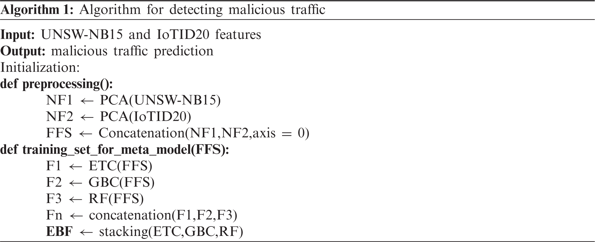
4 Proposed Extra Boosting Forest (EBF) Model and Architecture Flow
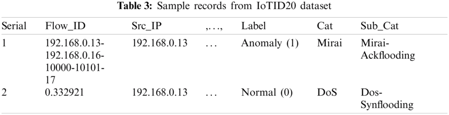
This study aims at detecting malicious traffic from the multi-domain dataset by developing a stacked ensemble model. Stacking is an ensemble method which aggregates predictions from multiple base-learners into one meta-predictor [43]. It mainly consisted of a 2-layer architecture where the first layer integrates all base-leaners and the second layer contains a meta-predictor which makes predictions of the base-learners to perform the final prediction [44]. A stacking model with m number of base-learners is trained similarly to k-fold cross-validation with each fold containing
and
Here, ETC, GBC, and RF are the base-learners with n trees. The new features set is generated using the probability of the base classifier's predictions and the size of the features set will depend on the size number of classes because the predicted probability for each class will be considered as a feature. So, the new features set for the training of meta leaner will be:
Here, D(M X N) is the new training set by the base models for the stack classifier and fp is the final prediction by the EBF. The architecture of the proposed model EBF is shown in Fig. 2.
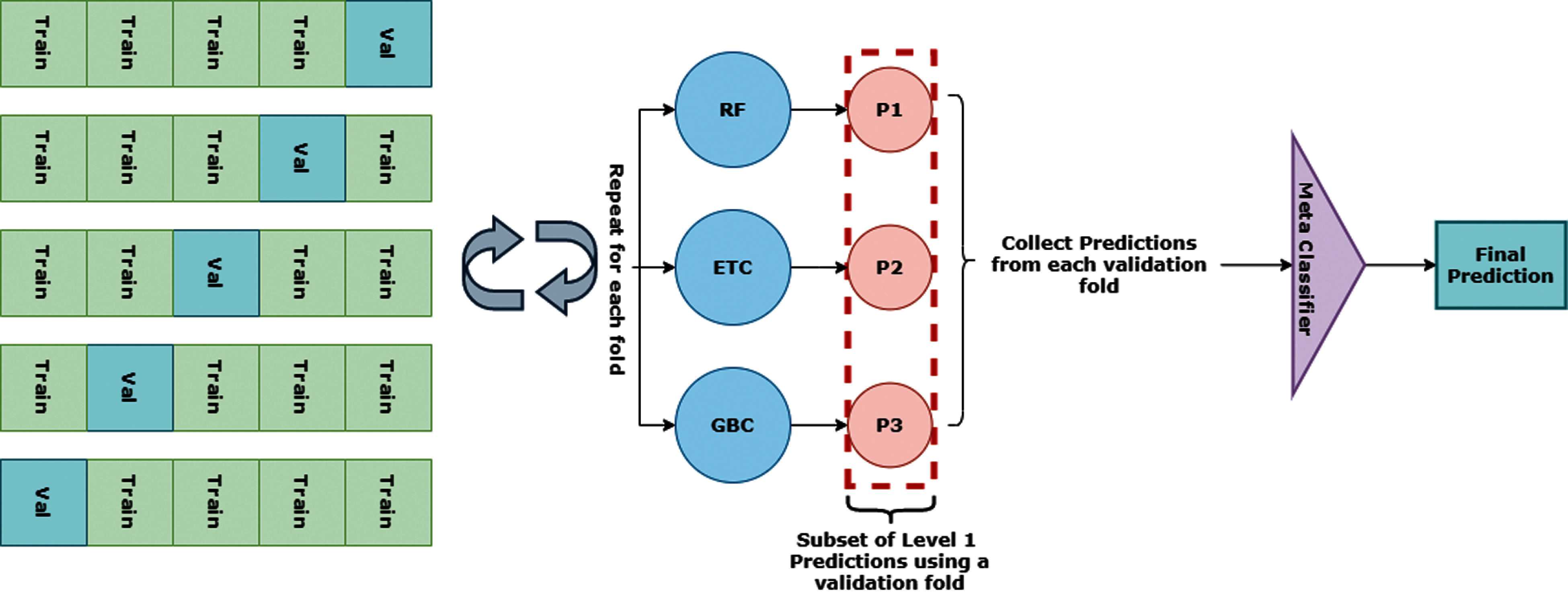
Figure 2: Architecture of the proposed EBF model
We proposed an ensemble model by combining the tree-based models such as extra tree classifier, gradient boosting classifier, and random forest. These models are selected based on their individual performances. In this regard, the top three best performers on both datasets are selected to make an ensemble model. Tree-based models perform well individually because targets in the datasets are not linearly separable, so tree-based models perform well as compared to linear models.
Figure 3: The illustration of horizontally merging of datasets using PCA features

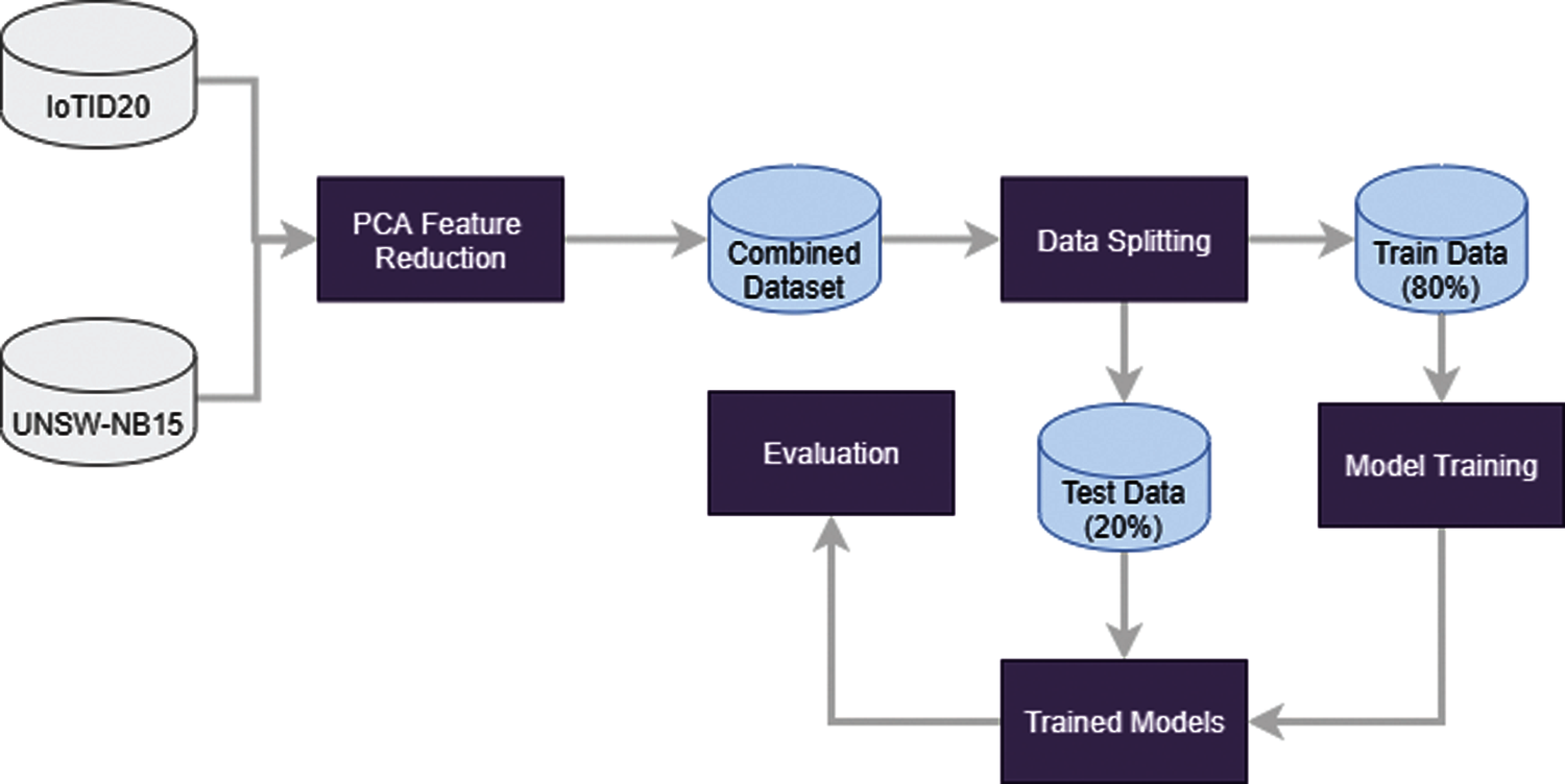
Figure 4: Flow architecture of the proposed methodology
This study focuses on the detection of malicious traffic from IoT traffic and local network traffic. For this purpose, we obtained two datasets from the publicly available repository. The dataset contains two target classes corresponding to network traffics records, as described in Section 3.1. To develop a more complex problem, we horizontally merged both datasets resulting in a multi-domain dataset. Equal numbers of features are required to merge the datasets, for which we used the PCA algorithm to select an equal number of features from each dataset. This PCA technique returns 30 features from each dataset which are further combined, as shown in Fig. 3.
We utilized 30,000 records from each target class from the IoTID20 dataset. The distribution of the total number of records in each dataset is shown in Tab. 6. After merging both datasets, we split the data into training and testing set with an 80:20 ratio. In the end, the evaluation of the trained models is carried out using several important performance evaluation metrics such as accuracy, precision, recall, and F1 score. The flow diagram of the proposed methodology is shown in Fig. 4.
The performance of machine learning models is evaluated on the network traffic datasets. Two approaches are followed, where initially the models are tested on individual datasets. Later, the training and testing are carried out using the merged complex dataset. Results for each approach are discussed in separate sections.
5.1 Performance of Machine Learning Models on IoTID20 Dataset
Experimental results of machine learning models on the IoT20 dataset are shown in Tab. 7. The tree-based machine learning models outperform other models concerning the evaluation metrics. DT, ETC, RF, and GBC achieved a 1.00 accuracy score against linear models whose performance is comparatively low. For example, LR and SGDC achieved 0.940 and 0.942 accuracy scores, respectively. On the other hand, the performance of KNN is marginally low than tree-based models with an accuracy of 0.99. Such high performance is attributed to the use and tuning of several important hyperparameters.

The performance of linear models is poor due to the distribution of class samples. Fig. 5 shows the class distribution for the IoTID20 dataset and it can be seen that the data samples are not linearly separable. Consequently, the performance of linear models has been degraded. Linear models perform better on the datasets where the data samples can be separated linearly which is not the case with the IoTID20 dataset.
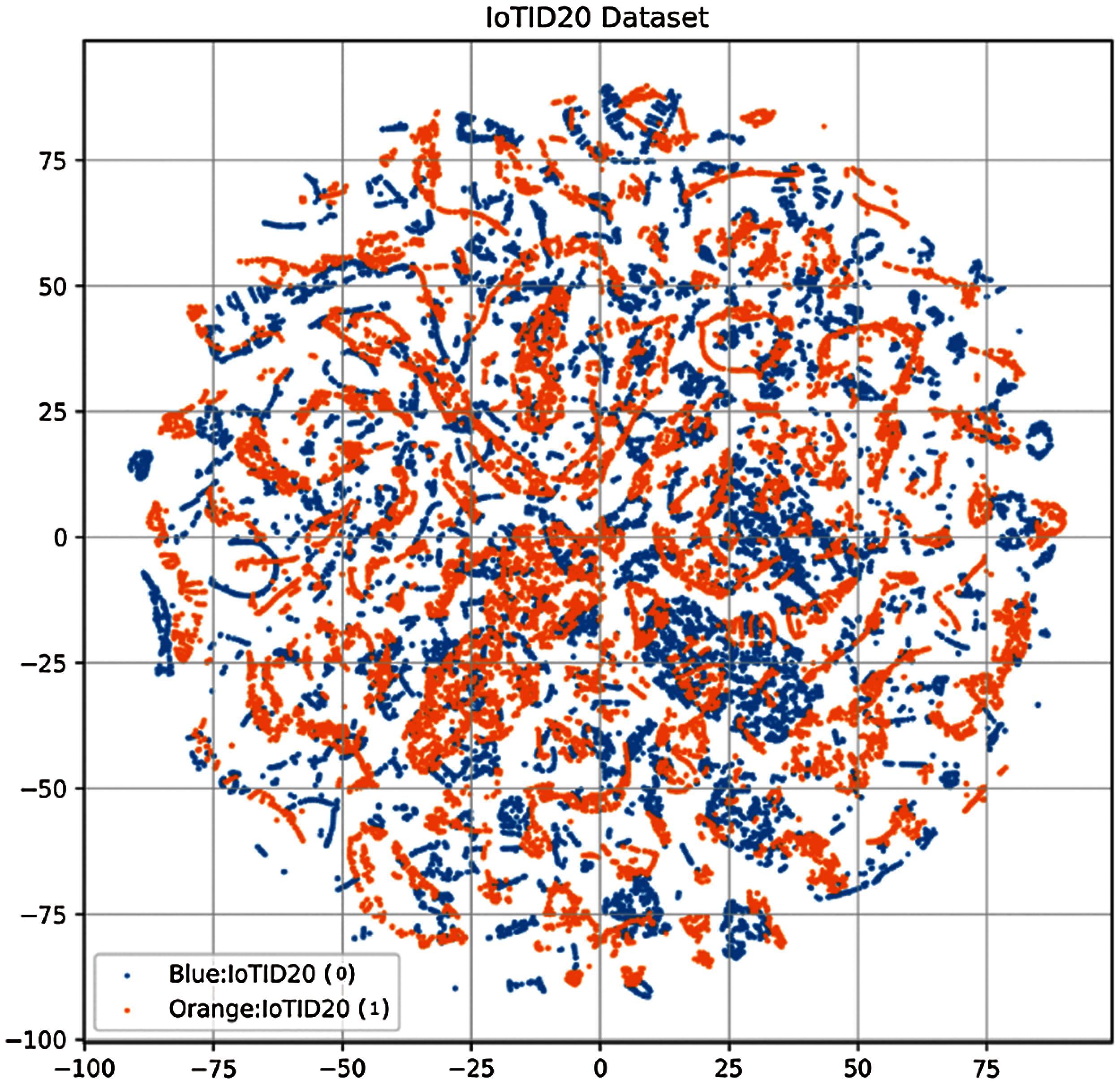
Figure 5: Class distribution for IoTID20 dataset
Tab. 8 shows the confusion matrix for models’ performance on the IoTID20 datasets where CP and WP correspond to correct predictions and wrong predictions, respectively. As discussed above, tree-based models perform exceptionally well, so the number of wrong predictions is zero. For KNN and linear models, several wrong predictions are made for each class. The highest number of wrong predictions is 1425 out of a total of 24,000 predictions from LR.
5.2 Performance of Machine Learning Models on UNSW-NB15 Dataset
Separate experiments are carried out using the selected machine learning models on the UNSW-NB15 dataset and results are shown in Tab. 9. The performance of tree-based models is also better on the UNSW-NB15 dataset where RF, ETC, GBC, and DTC achieve an accuracy score of 1.00. Conversely, the performance of linear models, as well as, KNN is substantially lower than that of tree-based models. The performance of linear models is low on UNSW-NB15 as compared to IoTID20 because the UNSW-NB15 has fewer features as compare to IoTID20 and the linear model sperform better when we have a large feature set that's the reason linear models perform better on the IoTID20 dataset. The performance of linear models is further reduced when used with the UNSW-NB15 dataset. GNB, SGDC, and LR achieve accuracy scores of 0.849, 0.735, and 0.923, while the accuracy of KNN is 0.898.


There are two possible explanations for the poor performance of linear models. First, as shown in Fig. 6 the data samples are grouped into different clusters which are not linearly separable. As a result, linear models are unable to find linear relationships among the data samples and show bad results. Secondly, the number of samples for the UNSW-NB15 is not equal. It has 45,332 and 37,000 samples for anomaly and normal classes, respectively. The imbalance of the training data further degrades their performance.
On the datasets tree-based models perform exceptionally well than other classifiers. Linear and probability-based models couldn't perform well because of non-linearity in data as shown in Tab. 10. Tree-based models are the best performer with 0 wrong predictions and KNN, GNB, SGDC, and LR perform poorly. SGDC gives the highest wrong predictions of 6,534 out of 24,700 predictions.
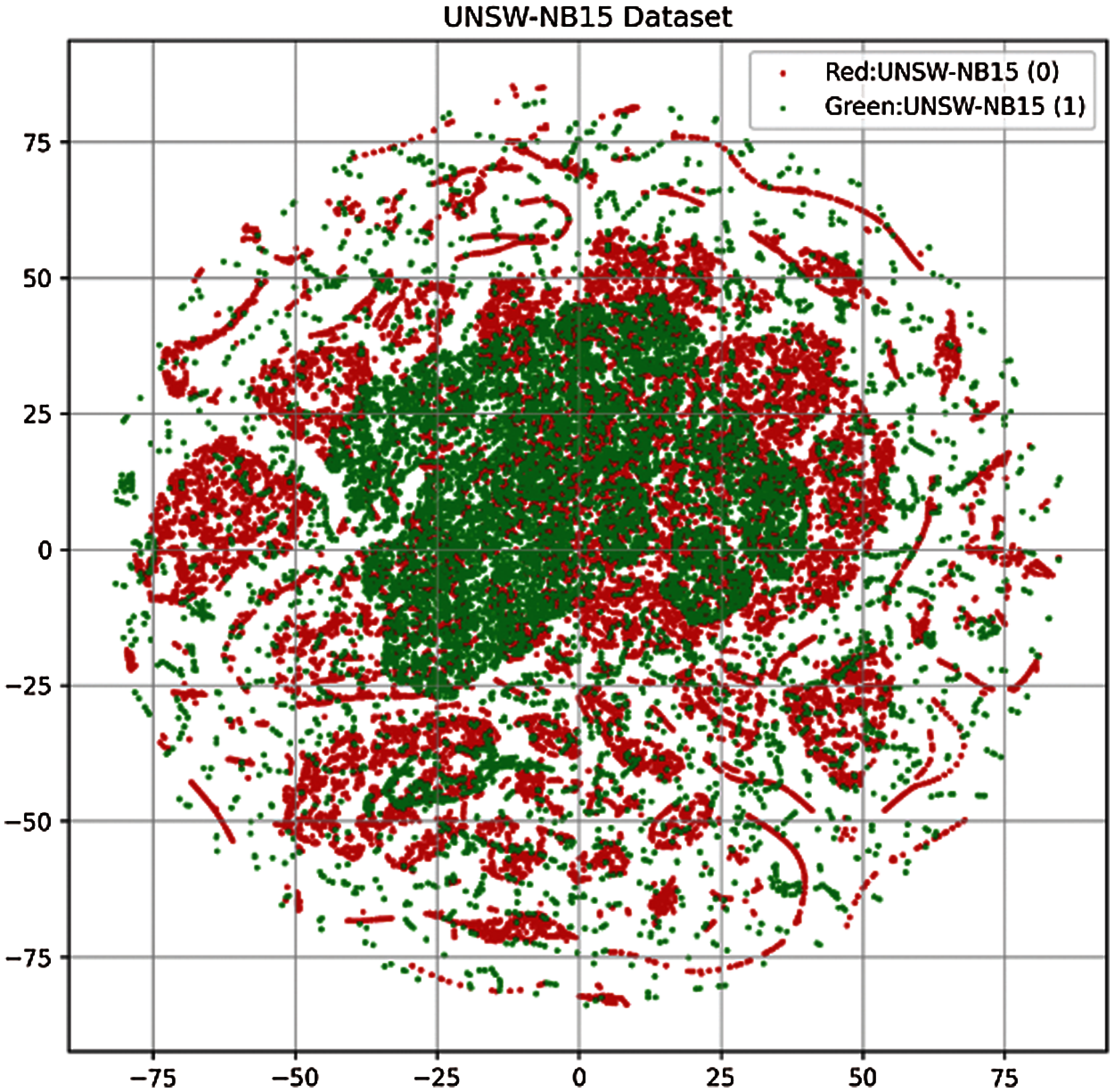
Figure 6: UNSW-NB15 dataset representation

5.3 Experimental Results of Machine Learning Models on Complex Dataset
The performance of models on individual datasets is good, however, the performance of the models needs to be analyzed with a complex dataset which is done by merging the dataset. After merging the datasets, the aim is to perform multi-class and binary classification. First, we have a binary classification problem where normal traffic and anomaly traffic data are considered for both datasets. For multi-class problems, we combine the data from UNSW-NB13 and IoTID20 datasets into four classes with normal traffic as 0 and 2 and anomaly traffic as 1 and 3 for UNSW-NB13, and IoTID20 datasets, respectively. The underlying objective is to detect the malicious traffic from IoT and local traffic networks using a single approach with high accuracy. The distribution of the dataset after combining two datasets is shown in Fig. 7.
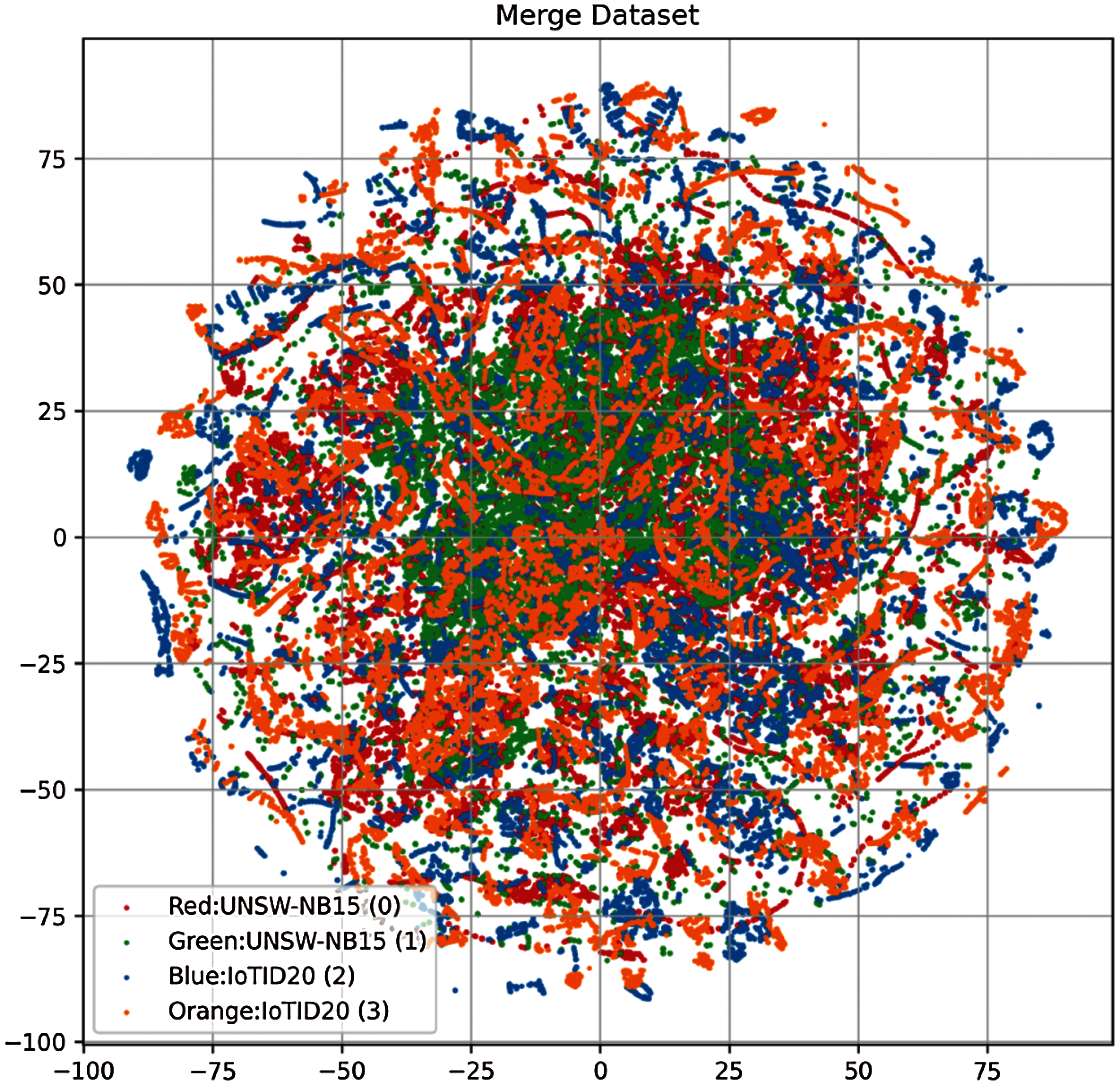
Figure 7: Distribution of the samples after merging the datasets
5.3.1 Performance of Machine Learning Models for Binary Classification
Experimental results shown in Tab. 11 show that the models show weak performance on the complex dataset. It is on account of merged features where the large feature set makes it difficult for the models to learn. The merging of datasets makes the experimental dataset complex as compared to the individual dataset, as Figs. 5–7 indicate. The target class correlation with features is different in individual and merged datasets. It becomes difficult for the machine learning models to have a good fit on a multi-domain dataset which affects the performance of the machine learning models. As a result, the models perform poorly with the complex dataset compared to their performance with each of the individual datasets. Even so, the performance of the tree-based model is superior to that of probability-based and linear models. So, RF gives the highest accuracy score of 0.981 while ETC and GBC are marginally behind RF with 0.978 and 0.986 accuracy scores, respectively.

Tab. 12 shows the correct and wrong predictions for all the models. As discussed above, the superior performance of tree-based models results in a lower number of wrong predictions with RF giving only 819 wrong predictions out of 42,700 total predictions. Linear models lack such performance due to a non-linear relationship among the data samples and show poor performance with SGDC giving the highest number of wrong predictions, i.e., 16,157 predictions out of 42,700 total predictions.

5.3.2 Performance of Machine Learning Models for Multi-Class Classification
Tab. 13 shows the results of selected machine learning models for four classes on the merged dataset. Results suggest that the performance of models has been degraded on multi-class classification. Tree-based models are still the leading performers for multi-class classification. Despite the decrease in their performance, there is a slight difference in the performance of binary and multi-class classification. On the contrary, the performance of linear models is severely affected. For example, the accuracy of SGDC and LR has been reduced to 0.460 and 0.649 from 0.621 and 0.711, respectively.

The number of CP and WP shown in Tab. 14 indicates that the GBC performs regarding correct predictions giving 41,893 correct predictions out of 42,700 total predictions. The performance of RF, ETC is very similar to that of GBC with 814 and 822 wrong predictions, respectively.

5.4 Performance of Proposed Stacked Model EBF
The performance of machine learning models is exceptional when tested on individual datasets, however, their classification accuracy is reduced when used with the complex dataset comprising the data from multiple domains. To increase the detection accuracy for malicious traffic, this study proposes EBF. The primary objective is to detect malicious traffic from multiple domain data with high accuracy. Several experiments are carried out to analyze the performance of the proposed EBF model. Initially, the performance of the proposed EBF model is evaluated on individual datasets and the results are shown in Tab. 15. Results show that EBF performs exceptionally well on the individual dataset with a 100% accuracy score which shows that our proposed model is significant for all scenarios.

Tab. 16 shows the experimental results on the multi-domain dataset for binary and multi-class classification. Results suggest that the performance of the proposed EBF is superior to other machine learning models. EBF achieves an accuracy of 0.985 for binary classification while the accuracy score for multi-class classification is 0.984 which is much better than other models. Another important point worth stating is the comparable performance of EBF for binary and multi-class tasks.

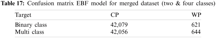
Tab. 17 shows the confusion matrix for EBF correct and wrong predictions. Statistics show that EBF has the lowest number of wrong predictions with 621 and 644 wrong predictions for binary and multi-class classification. It verifies that the performance of EBF is almost identical with two and four classes on the merged dataset.
To further corroborate the results of the EBF model, 10-fold cross-validation is performed using the merged dataset. Results of cross-validation are shown in Tab. 18 which indicates the superior performance of the proposed EBF model. Fig. 8 shows the significance of EBF on the binary and multiclass dataset.

5.5 Comparison with State-of-the-Art Approaches
The performance of the proposed EBF model is compared with several state-of-the-art approaches which used the same datasets. In comparison with previous studies, EBF performs well with the highest accuracy on the same datasets. Besides, these studies used either IoTID20 or UNSW-NB15 dataset individually, and experiments on the multi-domains dataset are not performed. In this regard, the experiments carried out in this study prove to be beneficial to realize the performance of machine learning models on multi-domain datasets. It also shows the superior performance of the proposed stacked model EF for its identical performance on binary and multi-class performance. Tab. 19 shows the accuracy comparison of EBF with state-of-the-art approaches on the same datasets.
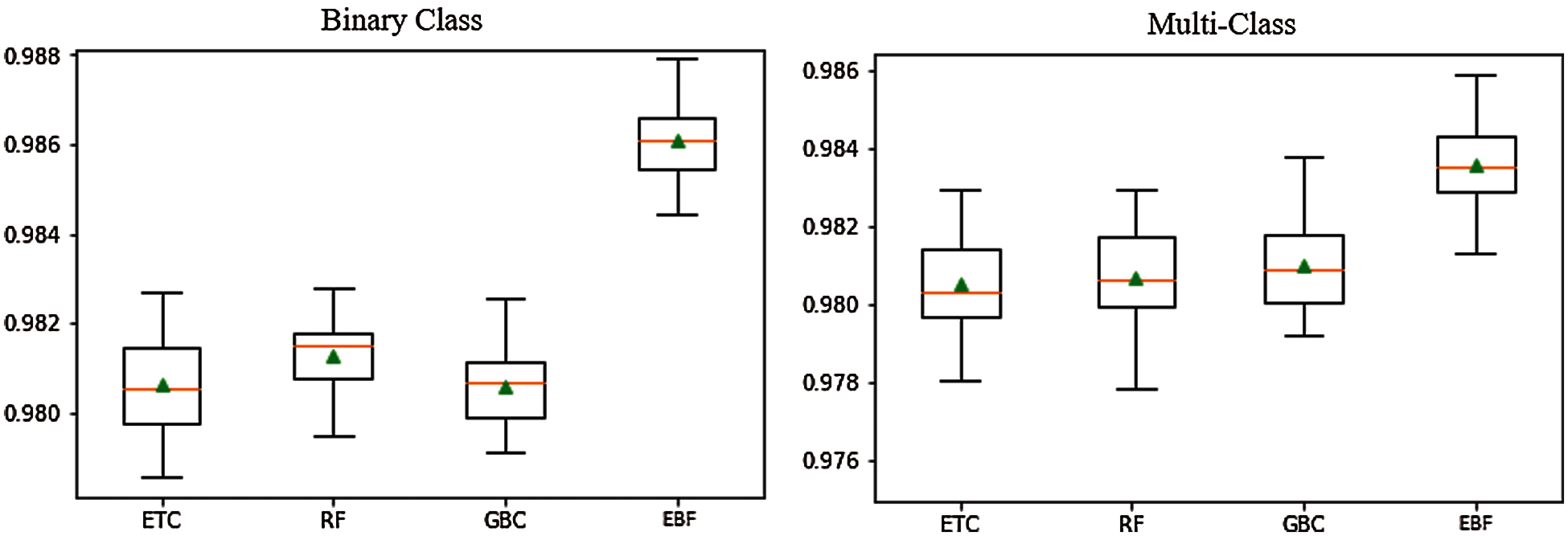
Figure 8: EBF performance using 10-fold cross-validation

5.6 Statistical Significance Test
To ensure the significance of our proposed model we have done the statistical T-test. Statistical T-test indicates if the difference in the performance of the proposed EBF model is statistically significant. To validate the test there are two hypotheses as follows [48]:
• Null hypothesis (Ho): There is a statistically significant difference between the proposed models and other models’ performances.
• Alternative Hypotheses (Ha): There is no statistical significance between models’ performance.
We implement a T-test on models’ performance and the T-test rejects H0 for EBF performance and other tree-based models on individual datasets and accepts Ha. It shows that the tree-based models and EBF perform equally well on the individual datasets, but it is statistically significant in comparisons to linear and probability-based models such as LR, GNB, KNN, and SGDC. When tested for the merged datasets, it accepts the H0 which means that the EBF is statistically significant as compared to all other models.
Malicious traffic detection from local and IoT networks is a very important task that holds great significance for the safeguard of network traffic. Although current automated systems can perform malicious traffic detection with higher accuracy, such models lack the ability to detect malicious traffic from multi-domain data. To overcome the limitations of existing methods, this study first analyzes the performance of machine learning models and then proposes a stacked model, called EBF, for the said task. For this purpose, experiments are performed on a complex dataset which is made by combining IoT-based dataset IoTID20 and local traffic dataset UNSW-NB15. Horizontally merging the datasets requires an equal number of features which is achieved by utilizing the PCA technique.
Experimental results indicate that traditional machine learning models perform better for individual datasets, however, their performance is degraded when tested with multi-domain datasets due to the complex features. Tree-based models perform better for malicious traffic detection while probability and linear models show poor performance due to the linear inseparability of the data. Furthermore, the performance of all the models is severely affected when tested for the multi-class problem. On the other hand, the proposed EBF model shows better results on the combined complex dataset because of its ensemble architecture. The performance of the proposed EBF model is superior to other models with 0.985 and 0.98 accuracy scores for binary and multi-classes, respectively. Besides, the performance analysis is carried out with several state-of-the-art approaches that used the same datasets for experiments. EBF outperforms these approaches on both single and merged datasets. In addition to that, the T-test and cross-validation suggest that the performance of the proposed EBF is statistically significant. Although this study performs experiments by combining two dataset, however, they both belong to IoT domain. Using the proposed approach on a different domain's data may affect the results substantially. To resolve this issue, we intend to perform additional experiments in future by integrating the data from several different domain and analyze the efficacy of the proposed approach.
Funding Statement: This research was supported by the Florida Center for Advanced Analytics and Data Science funded by Ernesto.Net (under the Algorithms for Good Grant).
Conflicts of Interest: The authors declare that they have no conflicts of interest to report regarding the present study.
1. C. Sinclair, L. Pierce and S. Matzner, “An application of machine learning to network intrusion detection,” in Proc. Annual Computer Security Applications Conf. (ACSACPhoenix, AZ, USA, pp. 371–377, 1999. [Google Scholar]
2. Y. Ye, D. Wang, T. Li and D. Ye, “IMDS: Intelligent malware detection system,” in Proc. Conf. on Knowledge Discovery and Data Mining (SIGKDDSan Jose, California, USA, pp. 1043–1047, 2007. [Google Scholar]
3. M. Shafiq, Z. Tian, A. K. Bashir, X. Du and M. Guizani, “Corrauc: A malicious bot-iot traffic detection method in iot network using machine learning techniques,” IEEE Internet of Things Journal, vol. 8, no. 5, pp. 3242–3254, 2020. [Google Scholar]
4. P. Sangkatsanee, N. Wattanapongsakorn and C. Charnsripinyo, “Practical real-time intrusion detection using machine learning approaches,” Computer Communications, vol. 34, no. 18, pp. 2227–2235, 2011. [Google Scholar]
5. C. F. Tsai, Y. F. Hsu, C. Y. Lin and W. Y. Lin, “Intrusion detection by machine learning: A review,” Expert Systems with Applications, vol. 36, no. 10, pp. 11994–12000, 2009. [Google Scholar]
6. Z. Xu, S. Ray, P. Subramanyan and S. Malik, “Malware detection using machine learning based analysis of virtual memory access patterns,” in Proc. Design, Automation & Test in Europe Conf. & Exhibition (DATELausanne, Switzerland, pp. 169–174, 2017. [Google Scholar]
7. L. Liu, B. S. Wang, B. Yu and Q. X. Zhong, “Automatic malware classification and new malware detection using machine learning,” Frontiers of Information Technology & Electronic Engineering, vol. 18, no. 9, pp. 1336–1347, 2017. [Google Scholar]
8. H. Rathore, S. Agarwal, S. K. Sahay and M. Sewak, “Malware detection using machine learning and deep learning,” in Proc. Int. Conf. on Big Data Analytics, Warangal, India, pp. 402–411, 2018. [Google Scholar]
9. M. Kalash, M. Rochan, N. Mohammed, N. D. Bruce, Y. Wang et al., “Malware classification with deep convolutional neural networks,” in Proc. IFIP Int. Conf. on new Technologies, Mobility and Security (NTMSParis, France, pp. 1–5, 2018. [Google Scholar]
10. D. Xue, J. Li, T. Lv, W. Wu and J. Wang, “Malware classification using probability scoring and machine learning, IEEE Access, vol. 7, pp. 91641–91656, 2019. [Google Scholar]
11. S. Euh, H. Lee, D. Kim and D. Hwang, “Comparative analysis of low-dimensional features and tree-based ensembles for malware detection systems,” IEEE Access, vol. 8, pp. 76796–76808, 2020. [Google Scholar]
12. M. Nisa, J. H. Shah, S. Kanwal, M. Raza, M. A. Khan et al., “Hybrid malware classification method using segmentation-based fractal texture analysis and deep convolution neural network features,” Applied Sciences, vol. 10, no. 14, pp. 4966, 2020. [Google Scholar]
13. J. Kang, S. Jang, S. Li, Y. S. Jeong and Y. Sung, “Long short-term memory-based malware classification method for information security,” Computers & Electrical Engineering, vol. 77, pp. 366–375, 2019. [Google Scholar]
14. B. Athiwaratkun and J. W. Stokes, “Malware classification with LSTM and GRU language models and a character-level CNN,” in Proc. Int. Conf. on Acoustics, Speech, and Signal Processing (ICASSPNew Orleans, LA, USA, pp. 2482–2486, 2017. [Google Scholar]
15. S. Sharma, C. R. Krishna and S. K. Sahay, “Detection of advanced malware by machine learning techniques,” Soft Computing: Theories and Applications, India, pp. 333–342, 2019. [Google Scholar]
16. G. Yan, N. Brown and D. Kong, “Exploring discriminatory features for automated malware classification,” in Proc. Int. Conf. on Detection of Intrusions and Malware and Vulnerability Assessment, Berlin, Germany, pp. 41–61, 2013. [Google Scholar]
17. B. Kang, S. Y. Yerima, K. McLaughlin and S. Sezer, “N-opcode analysis for android malware classification and categorization,” in Proc. Int. Conference on Cyber Security and Protection of Digital Services (Cyber SecurityLondon, UK, pp. 1–7, 2016. [Google Scholar]
18. M. Sewak, S. K. Sahay and H. Rathore, “Comparison of deep learning and the classical machine learning algorithm for the malware detection,” in Proc. Int. Conf. on Software Engineering, Artificial Intelligence, Networking and Parallel/Distributed Computing (SNPDBusan, Korea (Southpp. 293–296, 2018. [Google Scholar]
19. N. Moustafa and J. Slay, “UNSW-Nb15: A comprehensive data set for network intrusion detection systems (UNSW-NB15 network data set),” in Proc. Military Communications and Information Systems Conference (MilCISCanberra, ACT, Australia, pp. 1–6, 2015. [Google Scholar]
20. I. Ullah and Q. H. Mahmoud, “A scheme for generating a dataset for anomalous activity detection in IoT networks,” in Proc. Canadian Conf. on Artificial Intelligence, Ottawa, Ontario, pp. 508–520, 2020. [Google Scholar]
21. S. Karamizadeh, S. M. Abdullah, A. A. Manaf, M. Zamani and A. Hooman, “An overview of principal component analysis,” Journal of Signal and Information Processing, vol. 4, no. 3B, pp. 173, 2013. [Google Scholar]
22. M. Ringnér, “What is principal component analysis?,” Nature Biotechnology, vol. 26, no. 3, pp. 303–304, 2008. [Google Scholar]
23. H. Abdi and L. J. Williams, “Principal component analysis,” Wiley Interdisciplinary Reviews: Computational Statistics, vol. 2, no. 4, pp. 433–459, 2010. [Google Scholar]
24. G. Destefanis, M. T. Barge, A. Brugiapaglia and S. Tassone, “The use of principal component analysis (PCA) to characterize beef,” Meat Science, vol. 56, no. 3, pp. 255–259, 2006. [Google Scholar]
25. J. Shlens, “A tutorial on principal component analysis,” International Journal of Remote Sensing, vol. 51, no. 2, 2014. [Google Scholar]
26. H. S. Jo, C. Park, E. Lee, H. K. Choi and J. Park, “Path loss prediction based on machine learning techniques: Principal component analysis, artificial neural network and Gaussian process,” Sensors, vol. 20, no. 7, pp. 1927, 2020. [Google Scholar]
27. F. Song, Z. Guo and D. Mei, “Feature selection using principal component analysis,” in Proc. Int. Conf. on System Science, Engineering Design and Manufacturing Informatization, Yichang, China, vol. 1, pp. 27–30, 2010. [Google Scholar]
28. T. Howley, M. G. Madden, M. L. O'Connell and A. G. Ryder, “The effect of principal component analysis on machine learning accuracy with high dimensional spectral data,” in Proc. Int. Conf. on Innovative Techniques and Applications of Artificial Intelligence, Cambridge, UK, pp. 209–222, 2005. [Google Scholar]
29. W. Zhang, C. Wu, H. Zhong, Y. Li and L. Wang, “Prediction of undrained shear strength using extreme gradient boosting and random forest based on Bayesian optimization,” Geoscience Frontiers, vol. 12, no. 1, pp. 469–477, 2021. [Google Scholar]
30. D. Sun, J. Xu, H. Wen and D. Wang, “Assessment of landslide susceptibility mapping based on Bayesian hyperparameter optimization: A comparison between logistic regression and random forest,” Engineering Geology, vol. 281, pp. 105972, 2021. [Google Scholar]
31. C. C. Chern, W. U. Lei, K. L. Huang and S. Y. Chen, “ “A decision tree classifier for credit assessment problems in big data environments,” Information Systems and e-Business Management, vol. 19, no. 1, pp. 363–386, 2021. [Google Scholar]
32. S. Hakak, M. Alazab, S. Khan, T. R. Gadekallu, P. K. R. Maddikunta et al., “An ensemble machine learning approach through effective feature extraction to classify fake news,” Future Generation Computer Systems, vol. 117, pp. 47–58, 2021. [Google Scholar]
33. E. Winska, E. Kot and W. abrowski, “Reducing the uncertainty of agile software development using a random forest classification algorithm,” in Proc. Int. Conf. on Lean and Agile Software Development, Gdask, Poland, pp. 145–155, 2021. [Google Scholar]
34. S. L. Smith, B. Dherin, D. G. Barrett and S. De, “On the origin of implicit regularization in stochastic gradient descent,” in Int. Conf. on Learning Representation, Vienna, Austria, 2021. [Google Scholar]
35. Y. Deng and M. Mahdavi, “Local stochastic gradient descent ascent: Convergence analysis and communication efficiency,” in Int. Conf. on Artificial Intelligence and Statistics, San Diego, California, USA, vol. 130, pp. 1387–1395, 2021. [Google Scholar]
36. S. T. Nguyen, H. Y. Kwak, S. Y. Lee and G. Y. Gim, “Featured hybrid recommendation system using stochastic gradient descent,” International Journal of Networked and Distributed Computing, vol. 9, no. 1, pp. 25–32, 2021. [Google Scholar]
37. P. J. Chun, S. Izumi and T. Yamane, “Automatic detection method of cracks from concrete surface imagery using two-step light gradient boosting machine,” Computer-Aided Civil and Infrastructure Engineering, vol. 36, no. 1, pp. 61–72, 2021. [Google Scholar]
38. M. De Cock, R. Dowsley, A. C. Nascimento, D. Railsback, J. Shen et al., “High performance logistic regression for privacy-preserving genome analysis,” BMC Medical Genomics, vol. 14, no. 1, pp. 1–18, 2021. [Google Scholar]
39. S. Milanovi´c, N. Markovi´c, D. Pamuçar, L. Gigovi´c, P. Kosti´c et al., “Forest fire probability mapping in eastern Serbia: Logistic regression versus random forest method,” Forests, vol. 12, no. 1, pp. 5, 2021. [Google Scholar]
40. M. Kück and M. Freitag, “Forecasting of customer demands for production planning by local k-nearest neighbor models,” International Journal of Production Economics, vol. 231, pp. 107837, 2021. [Google Scholar]
41. A. Onyezewe, A. F. Kana, F. B. Abdullahi and A. O. Abdulsalami, “An enhanced adaptive k-nearest neighbor classifier using simulated annealing,“ International Journal of Intelligent Systems & Applications, vol. 13, no. 1, pp. 34–44, 2021. [Google Scholar]
42. A. X. Liu and R. Li, “K-nearest neighbor queries over encrypted data,” in Algorithms for Data and Computation Privacy, Cham: Springer International Publishing pp. 79–108, 2021. https://doi.org/10.1007/978-3-030-58896-0_4. [Google Scholar]
43. F. Rustam, A. A. Reshi, I. Ashraf, A. Mehmood, S. Ullah et al., “Sensor based human activity recognition using deep stacked multilayered perceptron model,” IEEE Access, vol. 8, pp. 218898–218910, 2020. [Google Scholar]
44. B. Pavlyshenko, “Using stacking approaches for machine learning models,” in Proc. Int. Conf. on Data Stream Mining & Processing (DSMPLviv, Ukraine, pp. 255–258, 2018. [Google Scholar]
45. A. Aleesa, M. Younis, A. A. Mohammed and N. Sahar, “Deep-intrusion detection system with enhanced unsw-Nb15 dataset based on deep learning techniques,” Journal of Engineering Science and Technology, vol. 16, no. 1, pp. 711–727, 2021. [Google Scholar]
46. M. Ahmad, Q. Riaz, M. Zeeshan, H. Tahir, S. A. Haider et al., “Intrusion detection in internet of things using supervised machine learning based on application and transport layer features using UNSW-NB15 data-set,” EURASIP Journal on Wireless Communications and Networking, vol. 2021, no. 1, pp. 1–23, 2021. [Google Scholar]
47. P. Maniriho, E. Niyigaba, Z. Bizimana, V. Twiringiyimana, L. J. Mahoro et al., “Anomaly-based intrusion detection approach for IoT networks using machine learning,” in Proc. Int. Conf. on Computer Engineering, Network, and Intelligent Multimedia (CENIMSurabaya, Indonesia, pp. 303–308, 2020. [Google Scholar]
48. M. D. Smucker, J. Allan and B. Carterette, “A comparison of statistical significance tests for information retrieval evaluation,” in Proc. ACM Conf. on Information and Knowledge Management, Lisbon, Portugal, pp. 623–632, 2007. [Google Scholar]
 | This work is licensed under a Creative Commons Attribution 4.0 International License, which permits unrestricted use, distribution, and reproduction in any medium, provided the original work is properly cited. |