Computers, Materials & Continua DOI:10.32604/cmc.2022.021804
Article

Extremal Coalitions for Influence Games Through Swarm Intelligence-Based Methods

Fabián Riquelme1,*, Rodrigo Olivares1, Francisco Muñoz1, Xavier Molinero3 and Maria Serna2

1Escuela de Ingeniería Informática, Universidad de Valparaíso, Valparaíso, Chile
2Computer Science Department, Universitat Politècnica de Catalunya, Barcelona, Spain
3Mathematics Department, Universitat Politècnica de Catalunya, Terrassa, Spain
*Corresponding Author: Fabián Riquelme. Email: fabian.riquelme@uv.cl
Received: 14 July 2021; Accepted: 19 August 2021

Abstract: An influence game is a simple game represented over an influence graph (i.e., a labeled, weighted graph) on which the influence spread phenomenon is exerted. Influence games allow applying different properties and parameters coming from cooperative game theory to the contexts of social network analysis, decision-systems, voting systems, and collective behavior. The exact calculation of several of these properties and parameters is computationally hard, even for a small number of players. Two examples of these parameters are the length and the width of a game. The length of a game is the size of its smaller winning coalition, while the width of a game is the size of its larger losing coalition. Both parameters are relevant to know the levels of difficulty in reaching agreements in collective decision-making systems. Despite the above, new bio-inspired metaheuristic algorithms have recently been developed to solve the NP-hard influence maximization problem in an efficient and approximate way, being able to find small winning coalitions that maximize the influence spread within an influence graph. In this article, we apply some variations of this solution to find extreme winning and losing coalitions, and thus efficient approximate solutions for the length and the width of influence games. As a case study, we consider two real social networks, one formed by the 58 members of the European Union Council under nice voting rules, and the other formed by the 705 members of the European Parliament, connected by political affinity. Results are promising and show that it is feasible to generate approximate solutions for the length and width parameters of influence games, in reduced solving time.

Keywords: Influence game; influence spread; collective behavior; swarm intelligence; bio-inspired computing

1  Introduction

Cooperative game theory deals with the study of players forming coalitions to achieve a common benefit, enforcing cooperative behavior [1]. Simple games are cooperative games where the benefit obtained by the coalitions is always binary, i.e., coalitions can either win or lose [2]. Simple games are one of the most fundamental models for decision-making [3], and have been used to solve problems arising voting systems, social choice theory, logic and threshold logic, circuit complexity, artificial intelligence, geometry, linear programming, Sperner theory, order theory, among other disciplines [3–5]. Besides the traditional forms of representation of simple games [6], since the 2010s, different formulations based on graphs have emerged, with the aim of applying the knowledge acquired in cooperative game theory in network science [7]. In this context, influence games arise as simple games defined by influence graphs (i.e., weighted, labeled graphs) on which an influence spread phenomenon is exerted. In an influence game, an initial activation of nodes (i.e., a coalition of players) is winning if it is able to influence at least a minimum number of nodes, called the quota of the game [8]. It is known that any simple game can be represented by an influence game, and vice versa [8]. Furthermore, influence games and influence graphs have been already used to solve problems of multi-agent systems [8], social network analysis [9,10], and collective decision-making models [11,12].

Despite the great expressiveness of influence games, it is a compact form of representation of simple games. Therefore, the computation of several parameters and properties coming from cooperative game theory on influence games is computationally hard (NP-hard, coNP-complete, or #P-complete) [8,11,12]. In the same vein, there are problems inherent to the influence spread phenomenon that are computationally hard. The best known is the influence maximization problem (IMP), one of the main problems of social network analysis [13]. This problem refers to finding k seed nodes in a network such that, under some influence spread model, the expected number of nodes influenced by the k seeds is the largest possible [14]. As a minimization problem, another possibility is to find the minimum seed set that allows influencing a given number of nodes [15]. This variation is also known as the least cost influence problem (LCI) [16].

Although the influence spread phenomenon was already studied in the 1970s to analyze collective behavior [17,18], its computational applications began to develop widely in the area of marketing in the early 2000s [19,20]. Two of the best-known general influence spread models are the linear threshold model (LT-model) and the independent cascade model (IC-model). For both, IMP and LCI turn out to be NP-hard [14,15]. Although the IC-model is often used more, due to its ease of implementation, as it is a predictive model, it produces less replicable results to experiment in case studies [8,21]. The high complexity of IMP and LCI makes it impractical to obtain optimal solutions through linear programming, integer programming, dynamic optimization, or other exact algorithms on networks with a large number of nodes. Therefore, since the 2010s different proposals have emerged to solve these problems in an approximate and efficient way. The solutions include greedy, approximation and community-based algorithms, heuristics, bio-inspired metaheuristics, among others [9]. Recently, a multi-objective optimization model was proposed to find the smallest set of nodes that can influence the largest number of nodes in the network [9].

In this work, we propose two optimization models inspired on [9] to find approximations to the length and width of an influence game. The length of a game is the size of the smallest winning coalition, while the width is the size of the largest losing coalition. Both parameters were firstly defined in 1990 as indicators of efficiency for decision-making [22]. The problems of computing the length and the width in an influence game are NP-hard [8]. As far as we know, this is the first time that both problems have been studied on influence games with a large number of players. As a case study, we compute the length and width of an influence game representing the simple majority voting system of the 705 members of the European Parliament, connected according to their political affinity. To face these case studies, we employ particle swarm optimization (PSO), which is a widely known swarm intelligence algorithm. The have three reasons to choose this technique over others: (a) any bio-inspired methods designed under the swarm collaborative behavior can be applied to this proposal; (b) PSO is one of the most popular optimizer algorithms, so there is extensive literature that reports its excellent efficiency [23]; and (c) it is a metaheuristic algorithm that has shown excellent performance to solve the similar IMP problem on which the formulation of the length and width approximation problems are based [21]. For the parameter adjustment of this optimizer, we will previously use a small case study of only 27 players, corresponding to the European Union Council under nice rules [24], in which we can compare the results with the exact solutions.

The article continues as follows. Section 2 presents the fundamental concepts related to influence games, along with the length and width of a game, and the influence maximization problem. Section 3 is devoted to model the optimization problems to approximate the length and the width of an influence game, and to present as well the bio-inspired metaheuristic algorithms used to solve those problems. In Section 4 we present the case studies, related with real voting systems. In Section 5, we show and discuss the results obtained by applying the models and methods defined in Section 3 to find approximations of the length and the width in influence games with a large number of nodes. Finally, Section 6 presents our main conclusions and future work.

2  Preliminaries

2.1 Influence Games

Here we use notation from [3,8]. A simple game is a type of cooperative game defined by a pair Γ=(N,W), where N is a set of players, and W is a monotonous family set on N, so that for all S,T⊆N, if S∈W and S⊆T, then T∈W. Any subset S⊆N is called a coalition (of players). W is the set of winning coalitions of the game. If a coalition does not win, it loses. L is the set of losing coalitions. Thus, W and L form a partition in such a way that W∩L=∅ and W∪L=P(N), where P(N) is the power set of N, i.e., the set formed by all the possible coalitions of the game. Wm is the set of minimal winning coalitions, i.e., those winning coalitions such that by removing any player we obtain a losing coalition. LM is the set of maximal losing coalitions, i.e., those losing coalitions such that by adding any player we obtain a winning coalition.

An influence graph is a tuple (G,w,f), where G=(V,E) is a graph (without loops) formed by a set of vertices V and a set of edges E⊆V×V. A weight function w:E→N assigns a value to each edge. The weight w(a,b) of an edge (a,b) represents the influence power exerted from a to b. A labeled function f:V→N assigns a value to each vertex. The label f(a) of a vertex a represents the resistance of a vertex to be influenced.

Influence graphs are structures on which different diffusion dynamics can be applied, determined by influence spread models. In an influence graph, the vertices can adopt two states, active or inactive, depending on whether or not they have been influenced through a certain influence spread model. In general, the idea is that from an initial set of vertex activation (the so-called seed), these vertices can be iteratively activating others in the graph or network until the active vertices can no longer continue to spread their influence. This iterative process stops when either all the network has been influenced, or there is not enough influence power to activate the remaining vertices. Note that the latter can be the case when the remaining vertices are not reachable from the active ones.

Formally, given an influence graph (G,w,f) and a seed or initial activation set X⊆V, the influence spread of X is the set F(X)⊆V formed by the nodes activated through an iterative process as follows. Lets Ft(X) denote the set of nodes activated at step t. Initially, at step 0, only the seed is active, so F0(X)=X. Then, at step i>0, the set of nodes activated is formed by all the nodes of Fi−1(X), plus some additional number of nodes that depends on the influence spread model. In this work we restrict us to the linear threshold model (LT-model) [20]. Under this model, in Fi(X) we add all the nodes whose labels are less or equal than the total weight of the edges pointing to them from nodes in Fi−1(X), i.e.,

Fi(X)=Fi−1(X)∪{v|∑{u∈Fi−1(X)|(u,v)∈E}w(u,v)≥f(v)} (1)

This process stops when no additional activation occurs. The final set of activated nodes is F(X)=Ft(X), where t=min{i∈N;Fi(X)=Fi+1(X)}≤|V|. Considering all the above, now we are able to define a form of representation of simple games based on influence graphs.

An influence game is a tuple (G,w,f,q,N), where (G,w,f) is an influence graph, q∈N is a quota and N⊆V is the set of players of the game. In case there are more nodes besides the players, then V∖N will be the set of auxiliary nodes. Thus, in an influence game, the set of winning coalitions is W={X⊆N;|F(X)|≥q}, and the set of losing coalitions is L={X⊆N;|F(X)|<q}. Note that influence games are an equivalent model to simple games, and therefore they retain the property of monotony, i.e., let X,Y⊆N, if F(X)≥q and X⊆Y, then F(Y)≥q. Henceforth, let be n=|N|.

2.2 Extremal Coalitions

In an influence game, minimal winning coalitions represent non-redundant alliances between players, such that each player is essential to “win” (by “win,” we mean passing a vote, adopting a product or service, making a collective decision, etc.). On the other hand, maximum losing coalitions are alliances that only need one more player to win. Despite the above, two minimal winning coalitions (or maximal losing coalitions) may have different cardinalities, so the coordination efforts required to be formed are different. Indeed, in a context of limited resources, we might be interested in forming an initial seed of players as small as possible, but with the ability to spread their influence to the other nodes in the network, in order to reach the necessary quota to win. Similarly, we might also be interested in knowing in advance what is the greatest wear or coordination effort to invest so as not to win the game. The latter would help us to know the inherent risk within the game. All the above leads us to the concepts of length and width of a game, as efficiency indicators for decision-making processes [22].

Let (G,w,f,q,N) be an influence game, then [8]:

•   The length of the game is the minimum size between the winning coalition of the game, i.e., min{|X|;X∈W}=min{|X|;|F(X)|≥q}.

•   The width of the game is the maximum size between the losing coalition of the game, i.e., max{|X|;X∈L}=max{|X|;|F(X)|<q}.

Sometimes, the width of a game is also defined as the minimum size of a blocking coalition [25], or as min{|X|;N∖X∈L}=min{|X|;|F(N∖X)|<q} (see also [26]). As this latter expression is equivalent to n−max{|X|;|F(X)|<q}, the results that we arrived at in this work could also be applied directly to those of this similar definition. The problems of computing the length and the width of an influence game are NP-hard [8].

2.3 Influence Maximization Problem

Let (G,w,f) be an influence graph, with a set of vertices V(G), and k∈N. The influence maximization problem (IMP) aims to select a seed X⊆V with |X|=k, that maximizes the influence spread F(X) through the network. In this work, we use the linear threshold model as the influence spread model. The best solution achieves |F(X)|=|V|.

Although we have worked with set notation so far, optimization problems often work with vector notation as well. In fact, a set X⊆{1,…,n} can be represented as a vector x=(1,…,n)∈{0,1}n, in such a way that X(x)={0≤i≤n;xi=1} and x(X)=(x1,…,xn)∈{0,1}n with xi=1 if i∈X, and xi=0 if i∉X [12]. For simplicity, we use undistingly x or X. We denote w(i,j)=wij for any edge (i,j)∈E(G). Thus, given an influence graph and k∈N, the IMP can be defined as the optimization of the following objective function:

s.t. ∑i=1nxi≤k (2)

A similar problem is the least cost influence problem (LCI), also known as target set selection problem (TSS) [27], which aims to minimize the seed X⊆V such that the influence spread F(X) achieves a given number of nodes k within the network, i.e., such that |F(X)|=k. Thus, the LCI can be defined as optimization of the following objective function.

s.t. |F(x)|≥k (3)

Although both IMP and LCI are NP-hard [14,15], there exist several efforts to find approximate solutions to these problems [21]. Both problems are closely related. As we already mentioned in Section 2.2, sometimes it is not enough to maximize the spread of influence, but it is also necessary to find a satisfactory seed. In this sense, by “satisfactory” we mean that it has a low cardinality of elements, and that it is minimal, i.e., if any actor i is removed from the seed, then |F(X∖{i})|<|F(X)|. In [21] a multi-objective model was defined to maximize the influence spread, while minimizing the seed size. This model was implemented using bio-inspired metaheuristic algorithms, with satisfactory results. Although, as we will see in Section 3, to calculate the length and width of a game will not be necessary to use multi-objective models, we will rely on the experience of [21] to compute these parameters in large games, for which the exact algorithms are not feasible.

3  Developed Solution

3.1 Optimization Models to Compute Extremal Coalitions

First, we define the length and width problems for an influence game using the integer programming paradigm. Given an influence game (G,w,f,q,N), the expression (4) details how minimal winning coalitions must be:

s.t. ∑i=1nxi≤|F(x)| (4)

while the expression (5) determines how maximum losing coalitions must be:

s.t. ∑i=1nxi≤|F(x)| (5)

Note that both optimization problems allow us to approximate extreme coalitions of a given game. The length corresponds to a global optimal solution for (4) which is also an optimal solution for (3). The width is a global optimal solution for (5). These metrics are not usually studied as combinatorial optimization problems. We remark again that computing the global optimal solutions for both problems on influence games is computationally intractable [8]. Note also that, unlike in [21], these problems are not multi-objective.

3.2 Swarm Intelligence Methods

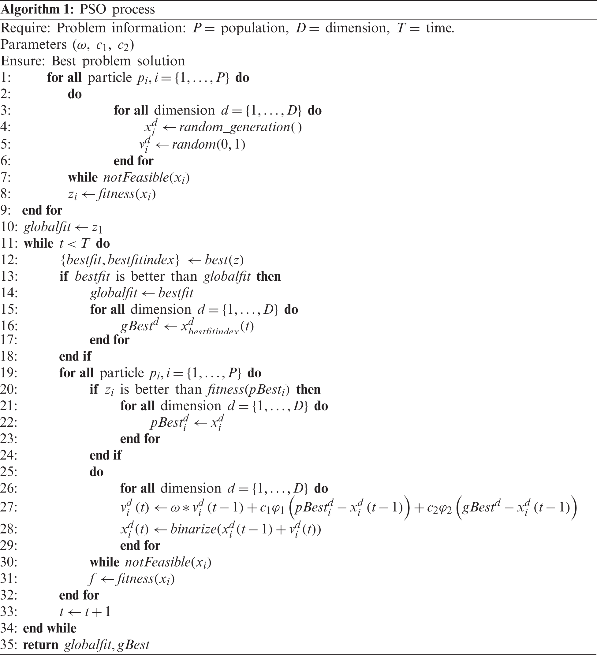
Swarm intelligence methods are a type of naturally bio-inspired metaheuristic algorithms. Like evolutionary algorithms, they are based on an initial population of possible solutions that improve over time. The swarm intelligence methods look for a common collective behavior between the particles that are part of this population. In this work, we use the particle swarm optimization method (PSO), which has already shown a correct performance for related problems [21].

The particles in PSO represent birds or fishes, each of which has two components: position and velocity. Each of these particles is a candidate solution. A set of particles forms a swarm, which evolves over time, where time is represented by discrete iterations. For each particle, the algorithm changes its velocity through the search space and then updates its position, depending on its own experience and the position of neighboring particles [28,29,23]. PSO has two well identifiable phases. In the initial phase, the particles increase their velocity so that current solutions lead to greater diversification. Once a high diversification is reached, the velocities progressively decrease to zero, and the second phase of intensification begins to search for more suitable solutions. This phase is executed in positions memorized as pBest. This memory capacity is precisely what allows PSO to continue improving its solutions over time. Therefore, the objective of the initial phase is to find pBest positions within the fittest attraction basins.

Velocity and position are represented by the vectors Vi=[vi1,vi2,…,viD] and Xi=[xi1,xi2,…,xiD], respectively. Initially, the particles are randomly positioned in a D-dimensional heuristic space with random velocity values. During the evolutionary process, each particle updates its velocity and position, according to the Eqs. (6) and (7), respectively:

vid=ωvid+c1φ1d(pBestid−xid)+c2φ2d(gBestd−xid) (6)

xid=xid+vid (7)

where d∈{1,…,D}, the positive constants ω, c1 and c2 are acceleration coefficients, φ1 and φ2 are uniformly distributed random numbers in the range [0,1], pBesti is the previous best position of ith particle, and gBest is the global best position found by all particles during the resolution process. A pseudocode that illustrates the entire PSO process is presented in Algorithm 1.

This algorithm allows solving both the length and the width problems. Section 4.3 explains how the functions of lines 4, 7, 28 and 30, were set. In lines 7 and 30, each time the domain of the particles is altered, its feasibility must be evaluated. These feasibility restrictions must be adapted to our context, so that they work for any influence game. Instead, the population generation (line 4) and the binarization process (line 28) must be adjusted on a case-by-case basis for each specific network or case study.

4  Voting Systems Experimentation

The main objective of this work is to apply the solution developed in Section 3 to find approximations to the length and width of influence games with a large number of players. As case studies, we consider real voting systems. In this context, players represent voters, and winning coalitions are sets of voters who can approve a law or amendment. Therefore, the quota of an influence game defines the minimum number of votes necessary to approve said law or amendment. As in [21], we first use a small case study on which the length and width can be computed by brute force. In this way, we fix the parameters of the metaheuristic algorithms to reach the ideal solutions. Then, with these parameter settings, we apply the algorithms to approximate the length and width of a much larger voting system, for which finding the exact solution is not feasible.

4.1 European Union Council Under the Nice Rules

The first case study corresponds to the qualified majority voting system of the Council of the European Union, modified by the Treaty of Nice in 2005 [24]. This simple game can be represented as an influence game (G,w,f,q,N), defined as follows:

•   G=(V,E) is a sparse, directed graph, with |V|=58 nodes and |E|=111 edges.

•   N={1,…,27} is formed by 27 member countries of the European Union (the players); hence, V∖N={28,…,58} are all auxiliary nodes.

•   Let be 1≤i≤27, 28≤j≤30 and 32≤k≤58. w(i,j) is the voting weight of player i in the weighted voting system j, w(j,31)=1, and w(31,k) =1 (see Appendix A).

•   The node labels are f(1)=…=f(27)=1, f(28)=255, f(29)=14, f(30)=620, f(31)=3, and f(32)=…=f(58)=1.

•   q=|V∖N|=31.

To see the formal details on the construction of this case study, see Appendix A. The resulting network is illustrated in Fig. 1.

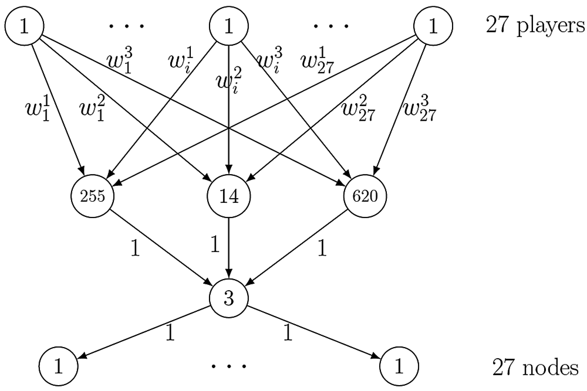
Figure 1: Influence graph for the EU council under the nice rules

4.2 European Parliament

The second case study corresponds to the majority voting system of the European Parliament (EP) in 2021. In this case, the EP is directly represented as an influence graph, corresponding to the social network of the different parliamentarians related by political affinity. To model this voting as an influence game, we must quantify the political affinity leading to the influence game (G,w,f,q,N) defined as follows:

•   G=(V,E) is a dense, undirected graph, with |V|=705 nodes and |E|=54488 edges.

•   N=V is formed by all the members of the EP. Each parliamentarian belongs to a country, a local political party (unless it is Independent), and a European political coalition (unless it is Non-Inscrits) associated with a political ideology (far-left, left, center-left, greens, center, center-right, right, far-right). In this case, there are no auxiliary nodes.

•   w:E→{1,2,3,4}. Given two players i and j, then w(i,j) represents the political affinity between both players. By default, w(i,j)=0 (i.e., the edge does not exist), unless:

•   both voters represent the same country;

•   both voters represent the same country and the same local political party;

•   both voters represent the same EP political group;

•   some of the two voters are “Non-Inscrits” but the political wing of both coincides (if some voter has no political wing, then it is not comparable with any other).

For each condition that is met above, add +1 to the edge between both players.

•   f:V→N∪{∞}. The label of each player node represents half (rounded down) +1 of the sum of edge weights pointing to the node (i.e., the simple majority criterion). A player i has f(i)=∞ (a large enough number) is there is no edge pointing to the node.

•   q=353, i.e., we use the simple or absolute majority criterion.

The whole dataset can be found in [30]. The resultant network is illustrated in Fig. 2. Note that this is a new social network defined for this specific work.

Figure 2: Social network for the European parliament: by countries (left) and by political tendency (right). The size of the nodes is in accordance with their degree

4.3 Implementation

All experiments were executed on a computer with an Intel Core i7-8700 processor, 32GB RAM 2666, 256GB SSD NVMe storage, on a 64-bit Windows 10 Pro operating system.

First, a brute force algorithm was implemented to calculate the length and width of an influence game given as input. The algorithm searches for all possible combinations of initial activations and determines its influence spread within the network, saving the smallest activations capable of reaching the quota (length) and the largest ones that do not reach the quota (width). This algorithm was run for the case study of the Council of the European Union presented in Section 4.1. The execution took 44 min. As a result, a width = 24 and a length = 14 was obtained. For the width, the following three optimal combinations were found (players are ordered according to Appendix A):

Solution 1: {2, 5, 6, 7, 8, 9, 10, 11, 12, 13, 14, 15, 16, 17, 18, 19, 20, 21, 22, 23, 24, 25, 26, 27}

Solution 2: {3, 5, 6, 7, 8, 9, 10, 11, 12, 13, 14, 15, 16, 17, 18, 19, 20, 21, 22, 23, 24, 25, 26, 27}

Solution 3: {4, 5, 6, 7, 8, 9, 10, 11, 12, 13, 14, 15, 16, 17, 18, 19, 20, 21, 22, 23, 24, 25, 26, 27}

For the length, 2317 optimal combinations were found. This big difference in the number of solutions should not be surprising because of the second weighted voting game considered in the case study (see Appendix A). All solutions were saved in a human readable file to identify the efficient solutions. Note that using this same algorithm for the European Union Parliament case study (Section 4.2) is intractable due to the large number of players. Therefore, we do not know the optimal solutions for this second influence game.

Second, PSO was implemented from the coding of [31], by following the structure presented in Algorithm 1. The new code is available in [30]. We performed previous executions to test different parameter configurations on a smaller case study in which the length and width can be computed by brute force. These preliminary experiments allowed us to study the parameter values of PSO, and which were later used for the toughest instances. Consistently, the best configuration was the already defined in [32]: c1=c2=1, φ1=φ2=Random(0,1), ω=1. A population of 25 individuals was used, 100 iterations each, allowing a total execution time of 9 s average for the length, and 1.5 s average for the width, reaching the best solution for all individuals (100% of the population). For this first case study, parallel programming was not required, and the convergences were found around the 25th iteration average. However, for the hardest case studies, multi-processing for particles (threads) was implemented in order to support the search process.

Third, the bio-inspired algorithms were executed on the second case study with the same parameter settings obtained from the first case study. The results are discussed in the next section.

For the feasibility constraint (lines 8 and 31 of Alg. 1) two cases are considered. For the length calculation, it was considered that the particle is feasible if fitness≥q; and for the width, if fitness<q, where fitness is the cardinality of the influence spread achieved, |F(x)|, and q is the quota of the given influence game. Regarding the population generation (line 4), a uniform distribution in [0, 1] was used for the length, and a uniform distribution with a domain bounded to [Φ−1,1] for the width, where Φ=(1+5)/2 is the golden ratio, so that Φ−1≈0.62. Finally, for the binarization function (line 28), sigmoidal functions were considered: for the length, the normal version random()<1/(1+e−x), and for the width, random()>1/(1+e−x).

Note that our proposal only works with feasible solutions, i.e., the solution vectors that do not satisfy the constraint, are not included in the swarm of solutions. To meet this requirement, a simple but powerful criterion of rejection is implemented. This method operates in a cycle way, each time a new solution is found. While a feasible solution is not reached, evolutionary changes depending on the algorithms are performed. This method seems to require an additional computational effort but in practice it is not. These computational experiments show it.

5  Results and Discussion

The results obtained for computing the length and the width in the case study of the network of European parliamentarians related by political affinity are presented and discussed below. To compute the length and the width, 60 executions were carried out in parallel. For the weight we considered 5000 iterations for each execution. For the length, we consider just 100 iterations, since the results were improving faster than for the weight.

5.1 Length of the European Parliament

Parallel executions of length all took around 900 s, that is, 15 min. The general results are shown in Tab. 1. Note that the values obtained for each row correspond to different executions, as they represent the “best” solutions of each type. In this context, the best solution found for the length is |x|=213. This is a winning coalition since it allows to spread its influence on |F(x)|=358≥353 players. Therefore, this hypothetical initial coalition x would allow influencing |F(x)|−|x|=145 new players, thus exceeding the necessary quota to win. Note also that these 213 players are only 30% of the total European MPs (members of the parliament), so it is indeed a rather small coalition.

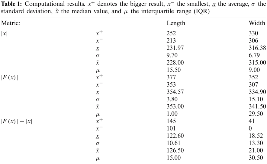
Fig. 3 presents a convergence plot for the best solution as the number of iterations progresses. The size of the coalition (initial activation |x|) for each iteration is represented by the red dotted line. Note that it never exceeds the quota of the game (q=353), and that it decreases continuously. The dashed blue line represents the spread of influence for the current coalition (i.e., |F(x)|). Although it has variations, it is never less than the quota. Therefore, from the first iteration, the coalitions accepted by the algorithm are always winners. On the other hand, in this case, it does not matter how much greater the reached spread of influence is, as long as it is greater than or equal to the quota. Therefore, the solid orange line representing the difference |F(x)|−|x|, in this case, is not so relevant.

5.2 Width of the European Parliament

Parallel executions of width all took around 11400 s, that is, 3.15 h. Although this is still a fairly low execution time (remember that computing the exact solution is intractable), it is much longer than for the length computation. This difference is because the solution space for width is much smaller than for length, or in other words, this game seems to have many more winning coalitions than losing coalitions. Therefore, PSO takes much longer between one iteration and the next to achieve a new improvement. This same reason was what led us to modify the randomization of the initial particles, described in Section 3.2; because the algorithm took a long time to find a particle that corresponded to a losing coalition (with a uniform random distribution, the initial particles turned out to be all winning coalitions).

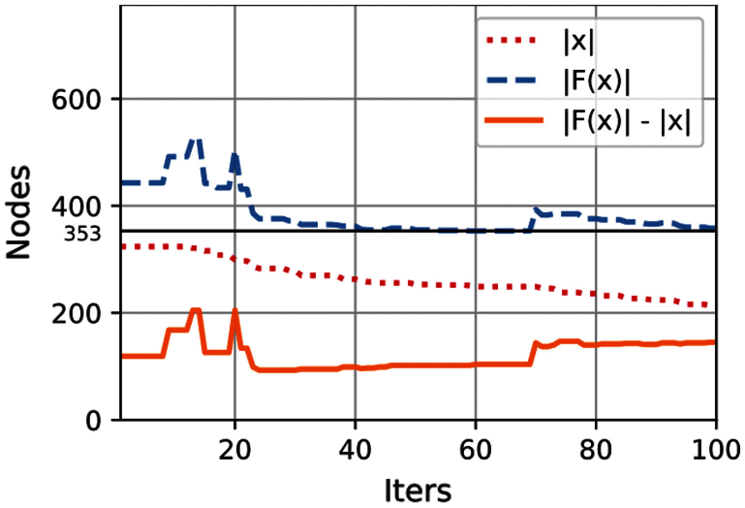
Figure 3: Best solution for the length computation

The general results are shown in Tab. 1. In this context, the best solution found for the width is |x|=330. There are two coalitions with this size. They are losing coalitions since they allow to spread its influence on |F(x)|=344 and |F(x)|=345<353 players, respectively. Therefore, although these hypothetical initial coalitions would allow influencing |F(x)|−|x|=14 or 15 new players, respectively, they cannot exceed the necessary quota to win. Note also that these 330 players are 44% of the total European MPs.

However, in this case, something different happens than in the length computation. Due to the monotony of the linear threshold model, note that the 14 or 15 players influenced by the best solutions could have been included as part of the initial activation. Thus, we would have an initial particle with |x|=345, which is still a loser, and whose difference is |F(x)|−|x|=0. This could be replicated for any other solution found with |F(x)|−|x|>0. Therefore, for the width computation, the largest value obtained for |F(x)|−|x| is relevant since it implicitly gives us a better approximation for the width. In this case, although the algorithm did not find a losing coalition of size 352 (47% of the total European MPs), we know that it exists, so this would be the value closest to the width of the game.

Fig. 4a presents the convergence plot for the solution with |x|=330 and |F(x)|=345. Furthermore, Fig. 4b shows the largest losing coalition obtained such that the difference with its spread of influence is zero, that is, the coalition such that |x|=|F(x)|=329. Although it is not clearly visible in the plots, both particles are subtly improving in the first iterations. The first solution converges in iteration 977, while the second, in iteration 3456. As for the length computation, in this case, the dotted red line never exceeds the quota (represented by the black line). However, here the curves are increasing. Additionally, the blue segmented lines are also kept below the quota.

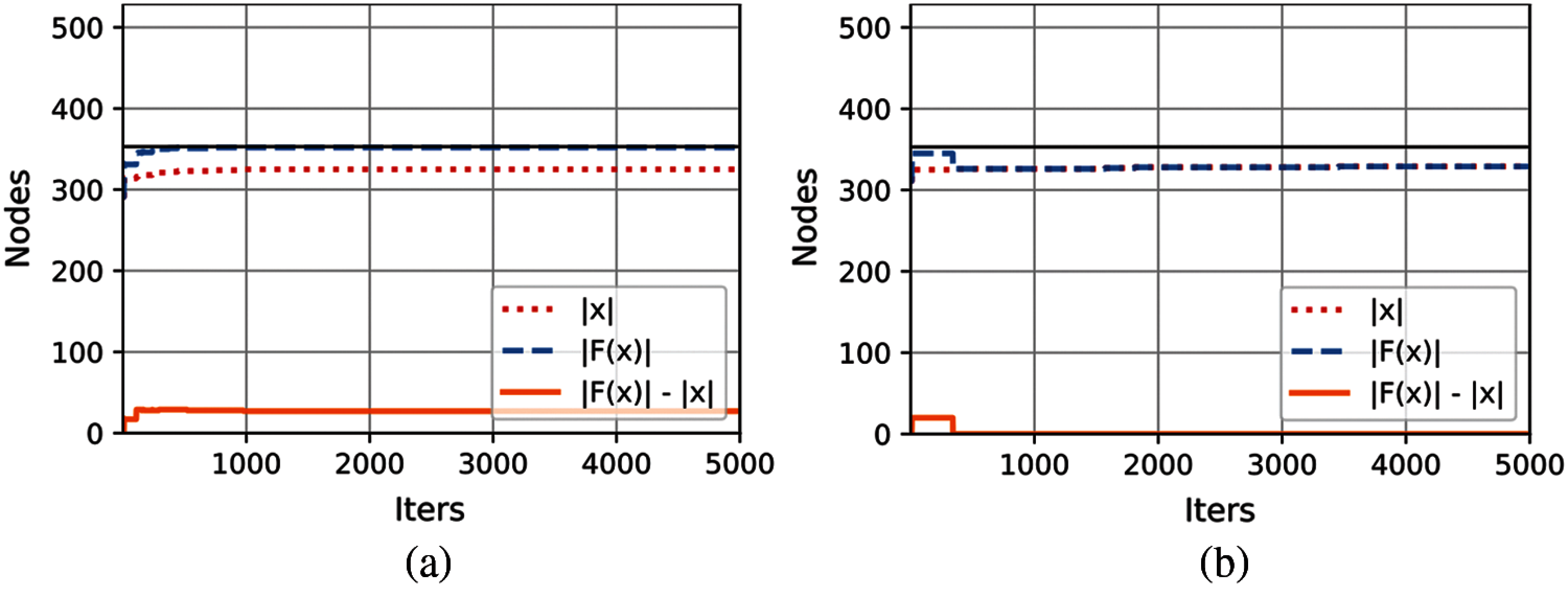
Figure 4: Best solutions for the width computation (a) Maximum losing coalition found (b) Maximum losing coalition without spread

6  Conclusions and Future Work

Many NP-hard problems, computationally intractable from a certain input size, can be solved by approximation algorithms, such as metaheuristics based on bio-inspired algorithms. These types of solutions, very common in graph theory, have been little explored to solve game theory problems. In this article, we use the PSO swarm intelligence algorithm to find efficient approximations for the length and width of an influence game. The modeling of these problems was based on other problems already known as the influence maximization problem. In cooperative game theory, influence games are a way to represent simple games as graphs or social networks.

As a case study, a social network formed by the 705 members of the European Parliament, related by political affinity, was considered. The best approximation for the length (i.e., the minimum winning coalition) was 213 players. Therefore, a coalition made up of only 30% of the parliamentarians was found, being capable of influencing another 145 players and thus exceeding the simple majority quota of 353 votes. For the width (i.e., the maximum losing coalition), two solutions of 330 members (44% of the parliamentarians) were found. These initial coalitions can influence a few additional players but still not capable of exceeding the game quota. Remarkably, in the case of the width, implicit solutions can be seen, given by the influence spread of the losing coalitions. As the higher influence spread found is 352, there is a coalition of 352 members, which is a loser and is not capable of influencing anyone else. Therefore, the best approximation of the width found for this case study is 352, although we do not know which players form this coalition.

Note that the solutions found include European MPs from different countries and political ideologies. As future work, ideological or country restrictions could be considered for the optimization problems (4) and (5). Thus, we could find the extremal coalitions made up of members of a certain political spectrum. This issue is beyond the original formulation of the length or width problems, but it would be useful from the point of view of voting theory and cooperative game theory.

Finally, we hope this approach could inspire new ways to solve game theory problems for larger instances than usual. In this sense, the problems representable as optimization problems are not few.

Funding Statement: F. Riquelme has been partially supported by Fondecyt de Iniciación 11200113, Chile, and by the SEGIB scholarship of Fundación Carolina, Spain; X. Molinero under grants PID2019-104987GB-I00 (JUVOCO); M. Serna under grants PID2020-112581GB-C21 (MOTION) and 2017-SGR-786 (ALBCOM).

Conflicts of Interest: The authors declare that they have no conflicts of interest to report regarding the present study.

References

 1.  R. Leonard, Von Neumann, Morgenstern, and the Creation of Game Theory: FromChess to Social Science, 1900–1960. Cambridge: Cambridge University Press, 2010. [Google Scholar]

 2.  J. von Newmann and O. Morgenstern, Theory of Games and Economic Behavior. Princeton, NJ: Princeton University Press, 1944. [Google Scholar]

 3.  A. Taylor and W. Zwicker, Simple Games: Desirability Relations, Trading, Pseudoweightings. Princeton, NJ: Princeton University Press, 1999. [Google Scholar]

 4.  T. Eiter, k. Makino and G. Gottlob, “Computational aspects of monotone dualization: A brief survey,” Discrete Applied Mathematics, vol. 156, no. 11, pp. 2035–2049, 2008. [Google Scholar]

 5.  K. Engel, Sperner Theory. New York, NY: Cambridge University Press, 1997. [Google Scholar]

 6.  X. Molinero, F. Riquelme and M. Serna, “Forms of representation for simple games: Sizes, conversions and equivalences,” Mathematical Social Sciences, vol. 76, no. 6, pp. 87–102, 2015. [Google Scholar]

 7.  G. Chalkiadakis, E. Elkind and M. Wooldridge, “Computational aspects of cooperative game theory,” in Synthesis Lectures on Artificial Intelligence and Machine Learning. Vol. 5, Williston: Morgan & Claypool Publishers LLC, pp. 1–168, 2011. [Google Scholar]

 8.  X. Molinero, F. Riquelme and M. Serna, “Cooperation through social influence,” European Journal of Operational Research, vol. 242, no. 3, pp. 960–974, 2015. [Google Scholar]

 9.  F. Riquelme, P. Gonzalez-Cantergiani, X. Molinero and M. Serna, “Centrality measure in social networks based on linear threshold model,” Knowledge-Based Systems, vol. 140, no. 3, pp. 92–102, 2018. [Google Scholar]

10. F. Riquelme, P. Gonzalez-Cantergiani, X. Molinero and M. Serna, “The neighborhood role in the linear threshold rank on social networks,” Physica A: Statistical Mechanics and Its Applications, vol. 528, no. 3, pp. 121430, 2019. [Google Scholar]

11. X. Molinero, F. Riquelme and M. Serna, “Satisfaction and power in unanimous majority influence decision models,” Electronic Notes in Discrete Mathematics, vol. 68, no. 2, pp. 197–202, 2018. [Google Scholar]

12. X. Molinero, F. Riquelme and M. Serna, “Measuring satisfaction and power in influence based decision systems,” Knowledge-Based Systems, vol. 174, no. 4, pp. 144–159, 2019. [Google Scholar]

13. D. Easley and J. Kleinberg, Networks, Crowds and Markets. Cambridge: Cambridge University Press, 2010. [Google Scholar]

14. D. Kempe, J. Kleinberg and É. Tardos, “Maximizing the spread of influence through a social network,” in Proc. of the ninth ACM SIGKDD Int. Conf. on Knowledge Discovery and Data Mining-KDD’03, Washington, D.C., ACM Press, pp. 137–146, 2003. [Google Scholar]

15. C. Long and R. C. W. Wong, “Minimizing seed set for viral marketing,” in 2011 IEEE 11th Int. Conf. on Data Minin, Vancouver, Canada, IEEE, pp. 427–436, 2011. [Google Scholar]

16. D. T. Nguyen, S. Das and M. T. Thai, “Influence maximization in multiple online social networks,” in 2013 IEEE Global Communications Conf. (GLOBECOMAtlanta, GA, IEEE, pp. 3060–3065, 2013. [Google Scholar]

17. M. Granovetter, “Threshold models of collective behavior,” American Journal of Sociology, vol. 83, no. 6, pp. 1420–1443, 1978. [Google Scholar]

18. T. Schelling, Micromotives and Macrobehavior. New York: Norton, 1978. [Google Scholar]

19. J. Goldenberg, B. Libai and E. Muller, “Using complex systems analysis to advance marketing theory development: Modeling heterogeneity effects on new product growth through stochastic cellular automata,” Technical Report, Academy of Marketing Science Review, 2001. [Google Scholar]

20. P. M. Domingos and M. Richardson, “Mining the network value of customers,” in Proc. of the Seventh ACM SIGKDD Int. Conf. on Knowledge Discovery and Data Mining, San Francisco, CA, USA, pp. 57–66, 2001. [Google Scholar]

21. R. Olivares, F. Muñoz and F. Riquelme, “A multi-objective linear threshold influence spread model solved by swarm intelligence-based methods,” Knowledge-Based Systems, vol. 212, no. 2, pp. 106623, 2021. [Google Scholar]

22. K. G. Ramamurthy, Coherent Structures and Simple Games. Dordrecht: Springer Netherlands, 1990. [Google Scholar]

23. D. Wang, D. Tan and L. Liu, “Particle swarm optimization algorithm: An overview,” Soft Computing, vol. 22, no. 2, pp. 387–408, 2017. [Google Scholar]

24. J. Freixas, “The dimension for the European union council under the nice rules,” European Journal of Operational Research, vol. 156, no. 2, pp. 415–419, 2004. [Google Scholar]

25. H. Aziz, “Algorithmic and complexity aspects of simple coalitional games,” Ph.D. thesis. University of Warwick, UK, 2009. [Google Scholar]

26. F. Riquelme, “Structural and computational aspects of simple and influence games,” Ph.D. thesis. Universitat Politècnica de Catalunya, Spain, 2014. [Google Scholar]

27. E. Ackerman, O. Ben-Zwi and G. Wolfovitz, “Combinatorial model and bounds for target set selection,” Theoretical Computer Science, vol. 411, no. 44–46, pp. 4017–4022, 2010. [Google Scholar]

28. J. Kennedy and R. Eberhart, “Particle swarm optimization,” in Proc. of ICNN’95-Int. Conf. on Neural Networks, Perth, WA, Australia, IEEE, pp. 1942–1948, 1995. [Google Scholar]

29. R. Eberhart and J. Kennedy, “A new optimizer using particle swarm theory,” in MHS’95. Proc. of the Sixth Int. Symp. on Micro Machine and Human Science, Nagoya, Japan, IEEE, pp. 39–43, 1995. [Google Scholar]

30. F. Muñoz, R. Olivares and F. Riquelme, “Swarm intelligence algorithms for width and length on influence games,” 2021. https://doi.org/10.6084/M9.FIGSHARE.14933259. [Google Scholar]

31. F. Muñoz, R. Olivares and F. Riquelme, “Swarm intelligence algorithms for multi-objective IMP,” 2020. [Google Scholar]

32. A. Nickabadi, M. M. Ebadzadeh and R. Safabakhsh, “A novel particle swarm optimization algorithm with adaptive inertia weight,” Applied Soft Computing, vol. 11, no. 4, pp. 3658–3670, 2011. https://doi.org/10.6084/M9.FIGSHARE.13046342. [Google Scholar]

Appendix A. European Union Council voting system as influence game

Let N={1,…,n} be a set of players. A weighted voting game (WVG) is a type of simple game that can be represented as a vector [q;w1,…,wn], where wi is the voting weight of player i, 1≤i≤n, and q∈N is a quota, such that a coalition X wins iff Σ{wi∣i∈X}≥q; otherwise, the coalition loses. Given m WVGs Γ1=[q1;w11,…,wn1], Γ2=[q2;wq2,…,wn2],…, Γm=[qm;wqm,…,wnm], their intersection Γ1∩Γ2∩…∩Γm forms a vector weighted voting game (VWVG), in which a coalition X wins if it wins in all WVGs separately; otherwise, the coalition loses. The European Union Council voting system under the Nice rules of 2005 can be represented as a VWVG formed by three WVGs [24]:

Let Γ=Γ1∩Γ2∩Γ3. It is known that every VWVG can be represented as an influence game [8]. For the case, the construction of Γ=(G,w,f,q,N) continues as follows (see Fig. 1):

•   The set of players N={1,…,27} is formed by the same players of Γ;

•   The vertex set V(G) is formed by N and 31 auxiliary nodes, so that V∖N={28,…,58};

•   The edges set E(G) is formed by the following. For all 1≤i≤27, 28≤j≤30 and 32≤k≤58, (i,j)∈E(G), (j,31)∈E(G), and (31,k)∈E(G).

•   The weight function w is defined as follows. For all 1≤i≤27, 28≤j≤30 and 32≤k≤58, w(i,j)=wij, w(j,31)=1, and w(31,k) = 1.

•   f(1)=…=f(27)=f(32)=…=f(58)=1, f(28)=255, f(29)=14, f(30)=620, f(31)=3.

•   q=|V∖N|=31.

Under this construction, note that a coalition (of players) wins iff it is capable of activates the auxiliary nodes 28, 29 and 30, i.e., iff the sum of weights reaches the quotas of the three WVGs. On the contrary, if one of the nodes 28, 29 and 30 can not be activated by a seed X, then it is not possible to activate the remaining 28 auxiliary nodes, and thus |F(X)|≤29<q, so X becomes losing.

This work is licensed under a Creative Commons Attribution 4.0 International License, which permits unrestricted use, distribution, and reproduction in any medium, provided the original work is properly cited.