Computers, Materials & Continua DOI:10.32604/cmc.2022.021747
Article

An Intelligent Forecasting Model for Disease Prediction Using Stack Ensembling Approach

Shobhit Verma1, Nonita Sharma1, Aman Singh2, Abdullah Alharbi3, Wael Alosaimi3, Hashem Alyami4, Deepali Gupta5 and Nitin Goyal5,*

1Computer Science & Engineering Department, Dr. B.R. Ambedkar National Institute of Technology, Jalandhar, India
2Computer Science & Engineering Department, Lovely Professional University, Jalandhar, India
3Department of Information Technology, College of Computers and Information Technology, Taif University, P. O. Box 11099, Taif 21944, Saudi Arabia
4Department of Computer Science, College of Computers and Information Technology, Taif University, P. O. Box 11099, Taif 21944, Saudi Arabia
5Chitkara University Institute of Engineering and Technology, Chitkara University, Punjab, India
*Corresponding Author: Nitin Goyal. Email: dr.nitingoyal30@gmail.com
Received: 12 July 2021; Accepted: 13 August 2021

This research work proposes a new stack-based generalization ensemble model to forecast the number of incidences of conjunctivitis disease. In addition to forecasting the occurrences of conjunctivitis incidences, the proposed model also improves performance by using the ensemble model. Weekly rate of acute Conjunctivitis per 1000 for Hong Kong is collected for the duration of the first week of January 2010 to the last week of December 2019. Pre-processing techniques such as imputation of missing values and logarithmic transformation are applied to pre-process the data sets. A stacked generalization ensemble model based on Auto-ARIMA (Autoregressive Integrated Moving Average), NNAR (Neural Network Autoregression), ETS (Exponential Smoothing), HW (Holt Winter) is proposed and applied on the dataset. Predictive analysis is conducted on the collected dataset of conjunctivitis disease, and further compared for different performance measures. The result shows that the RMSE (Root Mean Square Error), MAE (Mean Absolute Error), MAPE (Mean Absolute Percentage Error), ACF1 (Auto Correlation Function) of the proposed ensemble is decreased significantly. Considering the RMSE, for instance, error values are reduced by 39.23%, 9.13%, 20.42%, and 17.13% in comparison to Auto-ARIMA, NAR, ETS, and HW model respectively. This research concludes that the accuracy of the forecasting of diseases can be significantly increased by applying the proposed stack generalization ensemble model as it minimizes the prediction error and hence provides better prediction trends as compared to Auto-ARIMA, NAR, ETS, and HW model applied discretely.

Keywords: Disease prediction; stack ensemble; neural network autoregression; exponential smoothing; auto-ARIMA; holt winter

1  Introduction

The research community has been drawn to clinical databases for potential study and accurate forecasting, which allows people to take appropriate precautions to prevent future diseases. Time series forecasting techniques are frequently used to design forecasting systems for disease prediction through a collection of clinical datasets. These techniques discover patterns and trends in the time series data and use that in conjunction with the current year patterns to estimate the future occurrences [1]. Time series can be defined as a series of measurements for the time span selected. This time span may be equivalent to weekly, monthly, quarterly, annual, etc. [2]. A time series represents a series of t real value data is shown as Z1,…….,Zt, where Zi(1≤\; i\; ≤\; t) are the values recorded at a particular time i [3]. In addition to finding meaningful patterns in the data, time series forecasting techniques offer several advantages like reliability, able to find seasonal patterns, and trend estimations. On the Other Hand, these techniques suffer from the drawback of high generalization error of prediction. However, combining different forecasting models or the Ensemble model can be applied for reducing the generalization error and enhancing accuracy. Ensemble modeling is a metaheuristic way of combining different machine learning techniques to form a final forecast model to reduce variance and enhance prediction accuracy [4]. Ensemble converts multiple weak learners into single strong learner [5]. An ensemble model is primarily applied because of its capability in producing accurate results in different applications like classification or regression problems [6]. Following are the two main ways to perform ensembling for different models:

1.1 Sequential Ensemble Method

In this technique, the base learners are combined consecutively, wherein values obtained from previous model are used in the next model (e.g., AdaBoost), so the upcoming model handles error in the last model. Working of a sequential ensemble model can be illustrated in Fig. 1 [7].

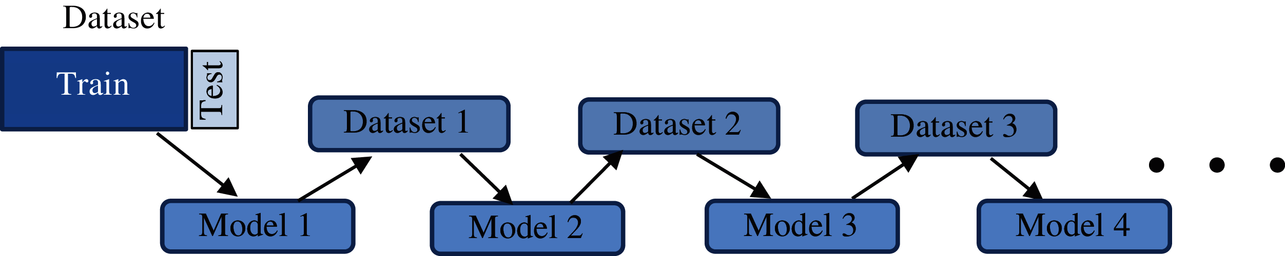
Figure 1: Sequential ensemble method

1.2 Parallel Ensemble Method

The base learners are produced in parallel i.e., side by side (e.g., Random Forest), and training data are provided to each model parallelly then combine all model result simultaneously. Working of a parallel ensemble model is shown in Fig. 2 [8].

One of the most widely used parallel ensemble model is stacking, where different classification or regression models are combined by a meta model [9]. It is essentially two-tier ensemble model, one is the base level (level 0) model that is trained on the entire training set, next is the meta (level 1) model which is trained over the outcomes of the base model [9]. It can be depicted in Fig. 3.

The manuscript proposes a stacked generalization ensemble model for time series forecasting techniques for prediction of number of incidences of Conjunctivitis disease. This research work proposes a meta learning approach i.e., stacking for robustly combining time series forecasting techniques that specializes them across the time series. The proposed model is applied on the conjunctivitis disease dataset and empirical results demonstrate the competitiveness of our model in contrast with the independent approaches for time series forecasting.

Figure 2: parallel ensemble methods

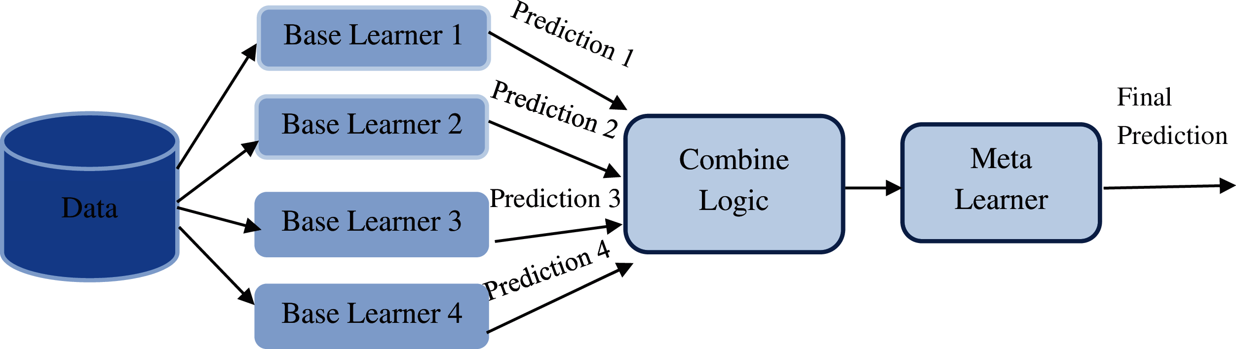
Figure 3: Stack ensemble model

Conjunctivitis is the conjunctiva inflammation, the thin and transparent tissue layer that forms inside the eyelid covering the eye's outer surface (white part or sclera) [10]. Each year, approximately 3 million cases occur in the United States. By dint of inflammation, the blood vessels in the conjunctiva become more visible that causes a reddish or pink appearance in the eye. It is mainly caused by viruses, bacteria (like Hemophilus influenzae and Streptococcus pneumoniae, etc.), allergic or immunological reactions, or by medicines. The symptoms of Conjunctivitis are itching in the eye, blur vision, swelling of the conjunctiva, gritty feeling in eye, pain, burning sensation in the eye, tearing, discharge in the eye that forms a crust at the time of sleeping which makes eyes to be stuck shut in the morning [11]. Conjunctivitis comes in many different forms, like Infective Conjunctivitis, Allergic Conjunctivitis, and Irritant Conjunctivitis [12].

Conjunctivitis is one of Hong Kong's most rudimentary ailments. Hong Kong's Department of Health and Government is carrying out many possible operations to avoid the possibility of future conjunctivitis disease. Many cases of conjunctivitis are still registered in Hong Kong city every week, even after the government's vital course of action. Hence, the advance prediction of future instances of conjunctivitis cases can help the government take pre-action to curb it. Time series forecasting techniques can be used to predict the future events of the same.

This manuscript aims to provide an ensemble model for evaluating and finding the most suitable method in estimating future instances of conjunctivitis disease. In this manuscript, the Conjunctivitis case dataset for the past few years is collected for analysis and forecasting, and initially, different time series forecasting models are applied to the data for future prediction of cases of conjunctivitis, and then a novel ensemble model is created with stack generalization technique. The research hypothesis is to generate a robust model based on diverse learners which can capture all the details of the time-series data and produce the accurate results. The base time series forecasting model to create the ensemble model are ETS, NNAR, Auto Arima, and Holt Winter, which are henceforth defined in the section on methodology.

In addition, each predictive model delivers different predictive outcomes depending on the dataset used. So, with various error metrics, the quality of the appropriate model is estimated. Error metrics that are used in this manuscript are as follows: RMSE, MAE, MAPE, and ACF, etc., details on the same is provided in the section on methodology [13].

2  Proposed Stack Generalization Ensemble Model

Fig. 4 shows the proposed ensemble model for conjunctivitis disease prediction. The proposed ensemble model is stack ensemble where three model are used as base models and one model as meta model [14]. Used Base models are auto Arima, NNAR and ETS, and with this used meta model is Holt Winter model.

Figure 4: Proposed stack generalization ensemble model

Working of proposed stack generalization ensemble model is described in the following steps:

Stack Generalization Ensemble Model

Input: Time Series Dataset as training (X) and testing (Y) dataset

Output: Forecasting of future occurrences (X^)

Step 1: Divide the Historical data for conjunctivitis is into train and test set.

Data=X+Y(1)

where X is train and Y is test data.

Step 2: Train each base model level 0 type (i.e., auto arima, NNAR and ETS) on train set.

Step 3: Find out the fitted values for auto arima, NNAR, ETS is given as:

X1=f1(X)+εta(2)

X2=f2(X)+εtb(3)

X3=f3(X)+εtc(4)

where X is training data, εta, εtb,εtc are errors generated by each model at time t respectively andX1, X2 and X3 are fitted values from model function f1(X), f2(X) and f3(X) respectively w.r.t. the model auto arima, NNAR and ETS.

Step 4: Fitted value from step 3 are passed to the stack generalizer which will calculate the mean of all fitted values. Let the mean of all fitted value is X¯, can be given as:

X¯=X1+X2+X33(5)

Step 5: The mean of fitted values calculated in step 4 with the help of stack generalizer will be given to level 1 meta model (i.e., Holt Winter model) as training set for train the model.

Step 6: Now forecasting is done from trained Holt Winter model, which can represent as:

X^=hw(X¯)(6)

where X^ is forecasted value on training data X¯ with hw() as Holt Winter model function.

Different models used in the Ensemble model are detailed as below:

2.1 Neural Network Auto Regression (NNAR/NAR)

A model based on the design and structure of the brain is known as an artificial neural network. It is said to be a smart model having the potential to acknowledge nonlinear features and time series-based patterns and then deal with the varied nonlinear relationship among dependent variables and its independent variable. The defining equation for the NNAR model can be given as follows, in which the target value for a neuron can be defined as shown in Eq. (7) [15]:

Z=fun(b+∑j⁡wjxj)(7)

where fun() is said to be the activation function of NAR, b is the bias of neuron, xj is the input variable, wj is the weight of neuron and Z depicts what the outcome of the model will be. Equation for predicted value can be given as Eq. (8) [15]:

y^(t)=f(y(t−1)+y(t−2)+……+y(t−p))+εt(8)

where y^ is predicted value ofy, f is a nonlinear function, y(t−p) previous vector time values and εt is the vector of random errors side.εt represents the error between the actual value and predicted value.

2.2 Auto ARIMA (Autoregressive Integrated Moving Average)

This model is the combination of AR (Auto Regression) model that predicts past values and MA (Moving Average) model [16] that makes a prediction on random error terms, and I stand of integration that is done to make it stationary. It can be written as: ARIMA (p, d, q) (P, D, Q) where p represents the AR order, d is differencing value, q is MA order, P,D,andQ represents the respective values for seasonal component.

Mathematically it can be written as:

φp(X)ΦP(XS)∇d∇SDZt=θq(X)ΘQ(XS)at(9)

where S represents the duration interval, φ implies AR parameter of order p, Φ represents seasonal AR parameter of orderP, Zt is observed value at t, θ is the MA operator of order q, Θ is the seasonal MA parameter of order Q, ∇d is the differencing operator, ∇SD is seasonal differencing operator and at at is the noise component [16].

2.3 Exponential Smoothing Model (ETS)

ETS model is special cases of ARIMA models. The latest observations are given exponentially more weight than older observations. ETS provides larger model class and each model is labeled as pair of (T,S) defining the type of ‘trend’ and ‘seasonality’, and it allows model selection via AIC (Akaike Information Criteria) i.e., triple exponential smoothing and all ETS models are nonstationary. It is a triplet (E,T,S) where E stands for error, T for trend and S seasonality components. It uses STLM (Seasonal adjustment) via STL (Cleveland-style loess).

2.4 Holt Winter Model

Holt Winter is a Simple Exponential Smoothing (SES) model with seasonal component. Holt Winter model comes under two special cases of ETS model class, which are:

(A,A): Holt-Winters’ additive method

(A,M): Holt-Winters’ multiplicative method

Above pairs show type of trend and seasonality respectively (i.e., T,S ) where A is for additive type and M is for multiplicative type.

Equations of additive Holt Winter are follows:

2.4.1 Level Component

Lt=α(yt−st−p)+(1−α)(Lt−1+bt−1)(10)

2.4.2 Trend Component

bt=β(Lt−Lt−1)+(1−β)bt−1(11)

2.4.3 Seasonality Component

st=γ(yt−Lt)+(1−γ)st−p(12)

2.4.4 Forecasting System

Yt+m=(Lt+bth)st−p+h(13)

where Yt is observed series, α, β and γ are the smoothing parameter (0≤α,β,γ≤1), Lt called as smoothed level at time t, bt is the change in the trend at time t, st is seasonal smooth at time t, p is the number of seasons per year, and h is the periods ahead forecast [17]. Holt-Winters model makes use of heuristic values for the starting state and then by optimizing the mean squared error (MSE), it calculates the smoothing parameter. In contrast to this ETS model optimizes the likelihood function for the evaluation of smoothing parameters as well as the initial states. As a result, it is seen that for a particular time series Holt-Winters gives improved result [17]. But in normal cases, ETS is preferred since it optimizes the starting states.

3  Materials and Methods

Fig. 5 depicts the outline of the time series forecasting methodology followed in this manuscript. Following steps are followed:

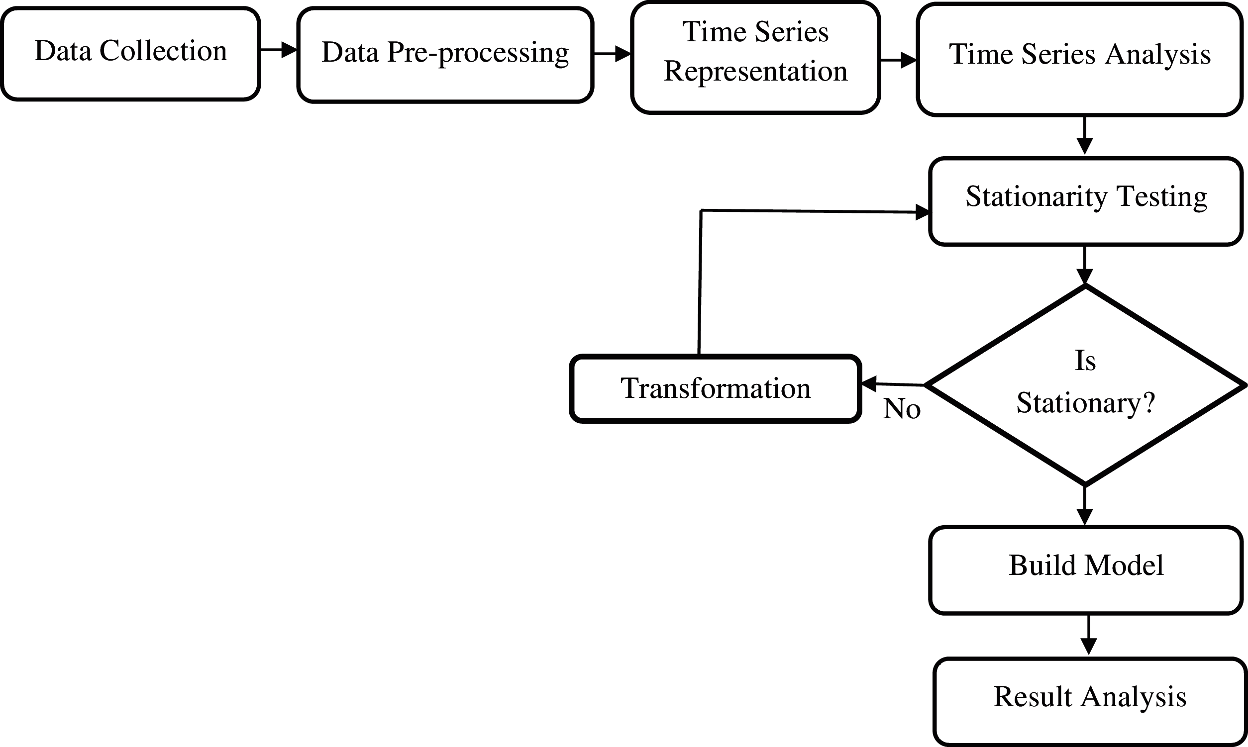
Figure 5: Methodology

3.1 Data Collection

The initial step is the collection of the disease data related to the conjunctivitis disease cases in Hong Kong city. Conjunctivitis cases weekly data is collected from the Hong Kong government website https://www.chp.gov.hk [18].

3.2 Data Preprocessing

The second step is data preprocessing, which deals with the mechanism of cleaning and imputation of the invalid or missing values by zero or by some value like median, mean, etc. [19]. Because data is in decimal number format so to make it a whole number, we multiply it by 10. So, before the weekly conjunctivitis cases were per 1000 and now become per 10000. In order to reduce the number of features, PCA and decision trees are applied.

3.3 Time Series Decomposition

The third step of the methodology is to convert conjunctivitis data into the form of time series. The time series formatted information holds a few imperative components, as explained below [19]:

3.3.1 Trend

It is also known as non-stationarity. It is mainly a long-term increasing or decreasing inclination of data. If the data contains a trend, then it should be eliminated from the data. Further, it can be of linear or nonlinear type. Linear trend represents the trend in a particular direction i.e., either increasing or decreasing, whereas in nonlinear trend changes do not follow a straight line. It is a mix of increasing and decreasing waves.

3.3.2 Heteroskedasticity

It mainly shows the randomness or irregularity of the data.

3.3.3 Seasonal Component

For fix and known time spam data show the same behavior, then data called seasonal data.

3.3.4 Stationarity

If the variance and the mean of the time series data is steady, then series known as stationary.

3.4 Time Series Analysis

The next step is to analyze the time series because a time series contains several types of patterns. So, to understand and analyze the time series, it is important to decompose the time series into its essential components. The three vital components of a time series are the trend-cycle, seasonality, and random or irregular [19]. Let yi is a time series with its three basic components. Accordingly, for additive time series and multiplicative time series, equations are given in Eq. (14) and Eq. (15)

yi=Si+Ti+Ei(14)

For equation can be represented as:

yi=Si×Ti×Ei(15)

where yi is time series data at the period i, Si is a seasonal factor, Ti is trend-cycle, and Ei is the reminder components at periodi .

3.5 Stationarity Testing

The next step is stationarity testing that checks the stationarity or non-stationarity of the time series, which is performed with the help of L-Jung and Augmented Dickey-Fuller (ADF) tests, and further, if time series is found to be stationary then time series forecasting model can be directly applied otherwise, there is need for conversion of the nonstationary series into stationary one. If there is a time series as Zt(t=1,…..,n), then it will be stationary when its mean and variance are constant and its auto covariances does not depend on time t [20]. Non-stationary time series can be converted into stationary by different types of processes such as smoothing, transformation and differencing. The need for transforming the variable is to stabilize the variance or mean. logarithmic transformation [2/0] is used here to reduce the variances of conjunctivitis time series and to make it stationary, it can be described as Eq. (16):

y=log⁡(x)(16)

3.6 Model Building

The last step involves the application of the proposed model on the time series data. The stacked generalization ensemble model as described in previous section works in two phases. In the first phase, three models namely auto arima, NNAR and ETS are applied. The result of these models is averaged and passed to the meta learner. After those predictions are made and finally the results are evaluated based on error metrics explained below:

3.6.1 Root Mean Squared Error (RMSE)

RMSE is evaluated as the square root of the average of square of difference in predicted and actual values and formula can be defined as Eq. (17) [21].

RMSE=∑i=1n⁡(xi−x)2n(17)

3.6.2 Mean Absolute Error (MAE)

MAE is measure of error, which is the mean of the absolute error, that is the average of forecasting error without direction. Forecasting error if calculated by the difference of actual and predicted values.

MAE=1n∑i=1n⁡|xi−x|(18)

3.6.3 Mean Absolute Percentage Error (MAPE)

It is measuring the magnitude of error compared to the magnitude of actual data, as a percentage. For measuring the accuracies of forecasted data, MAPE is used. It is also known by the name of Mean Absolute Percentage Deviation (MAPD). MAPE is average of absolute percentage error, depicted in Eq. (19) as:

MAPE=1n∑i=1n⁡|xi−xx|×100(19)

3.6.4 Auto Correlation Function (ACF) Error

It is also a means to find accuracy which depicts the interrelationship of actual time series with time series of lag 1.

ACF1=1n(1+2∑i=1k−1⁡(xi−x)2)(20)

4  Result and Discussion

In this manuscript, a statistical tool called R is employed for the Conjunctivitis disease forecasting. Conjunctivitis data are taken from the Hong Kong website of “The Centre for Health Protection, Department of Health” (https://www.chp.gov.hk). Collected information tells the weekly rate per 1000 of Acute Conjunctivitis of GOPC (General Out-patient Clinics) and PMC (Private Medical Practitioner) Clinic for the duration of 8 years and 1 month i.e., from the first week of January 2010 to last week of December 2019. Here in this data, the sum of GOPC rate and PMPC rate per 1000 is taken as a univariate variable. Then the preprocessing i.e., cleaning, and imputation process applied on Hong Kong conjunctivitis data and because data is in decimal number format so to make it a whole number, it is multiplied by 10. So, before the weekly conjunctivitis cases were per 1000 and now it becomes per 10000. Further, the data is divided into two parts i.e., training and testing in the fraction of 88% and 12% respectively. So, conjunctivitis data from the first week of 2010 to last week of 2017 is taken as training dataset and rest part of data as the testing dataset. After that data is converted in time series objects like ts_conjunctivitis_data, train_ts and test_ts objects for the total conjunctivitis data, training data and test data respectively. Then after this time series conversion, the time series was plotted. Fig. 6 show the time series plot of conjunctivitis data.

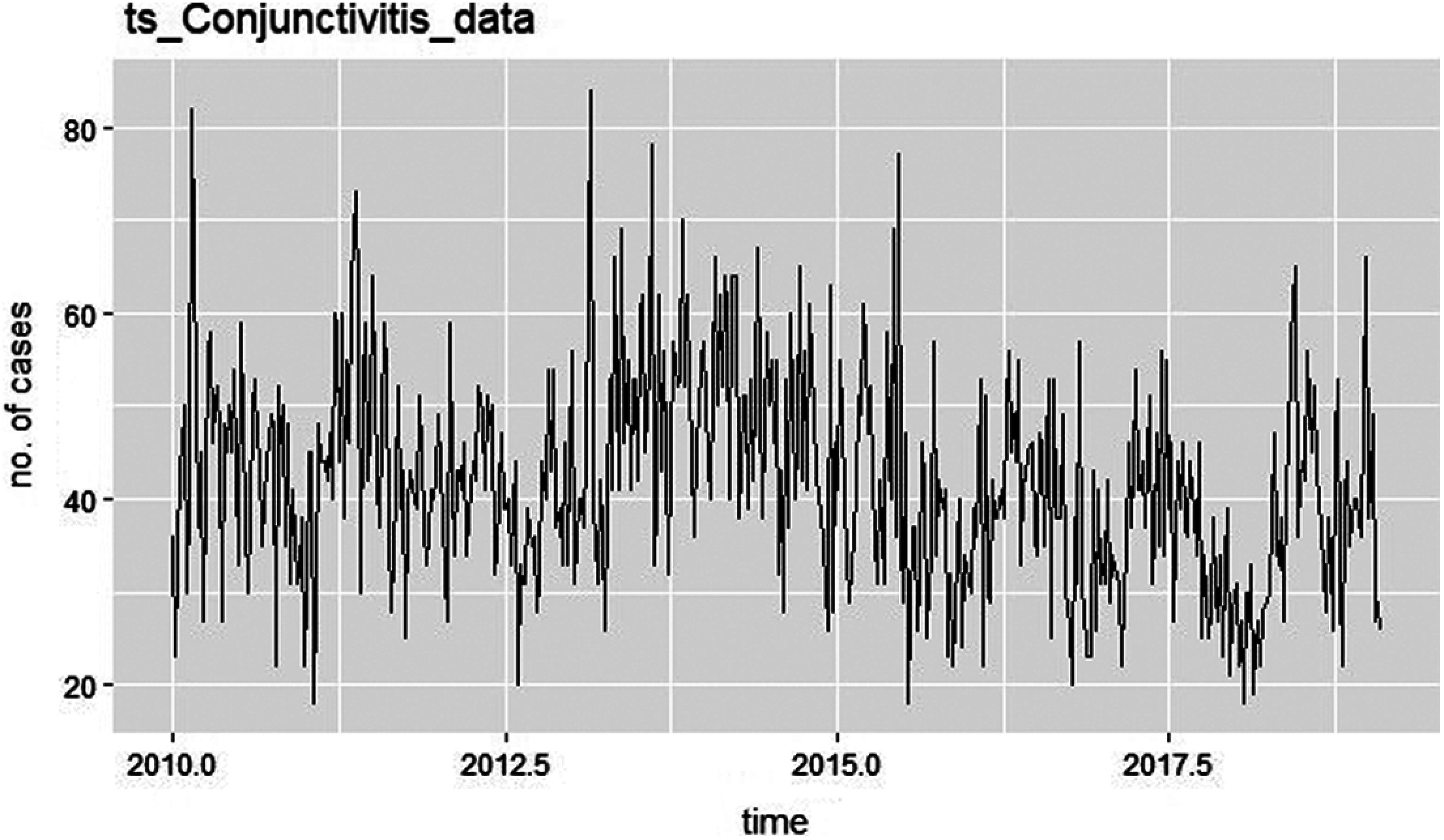
Figure 6: Time series plot of conjunctivitis data

Then for time series analysis purpose, decompose the time series into its essential components to see the trend and seasonality, the graph for the same is given in Fig. 7.

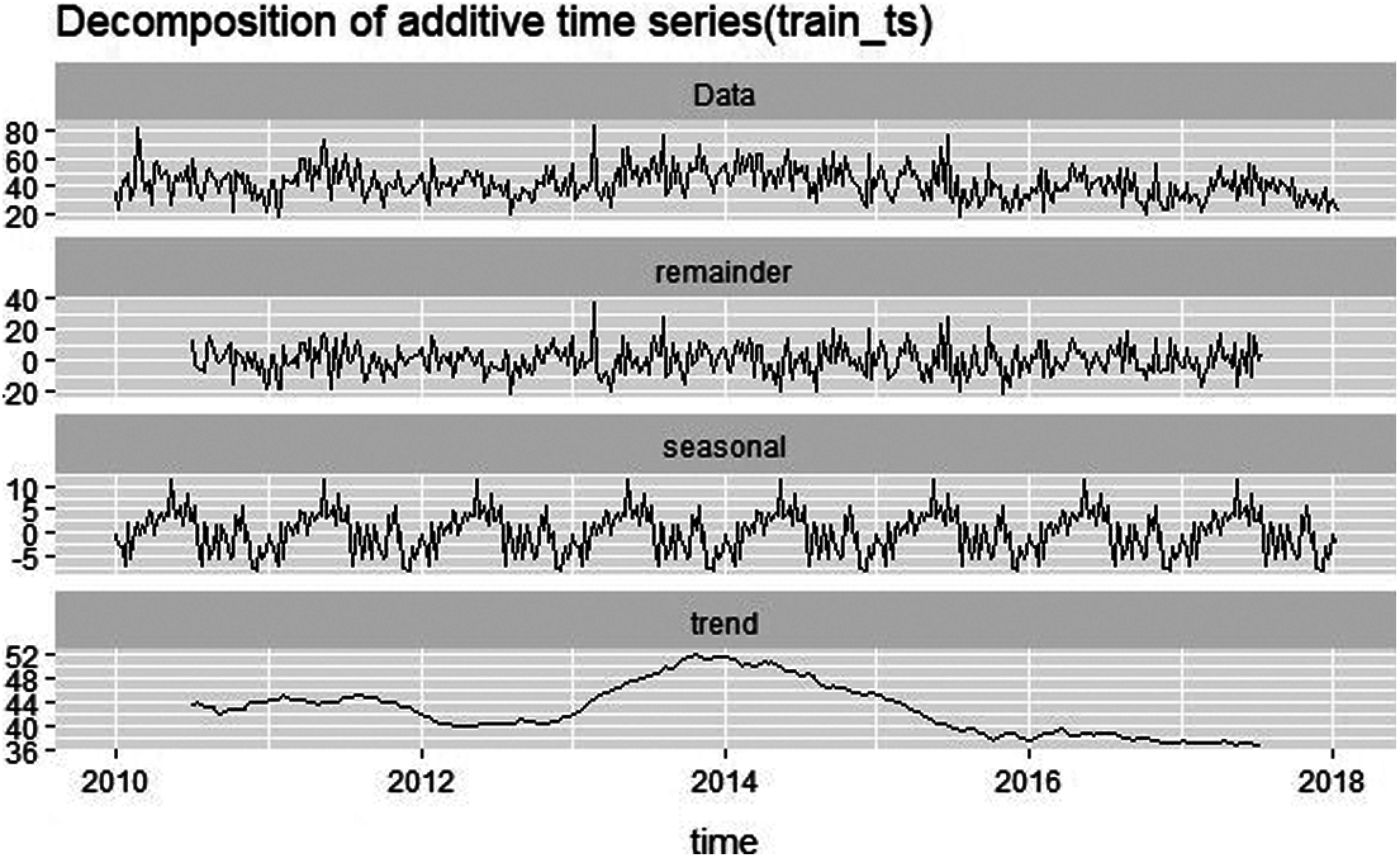
Figure 7: Decomposition plot of training data

As demonstrated in the above-mentioned graph, it is evident that the time series plotted in the graph has elements of trend and seasonality, therefore we can easily conclude that the series is non-stationary. That necessitates us to convert to a stationary one. The conversion of non-stationary series into a stationary is done by logging the series using the log()function. Fig. 8 shows the time series plot of training data with log i.e., plot of log⁡(train_ts).

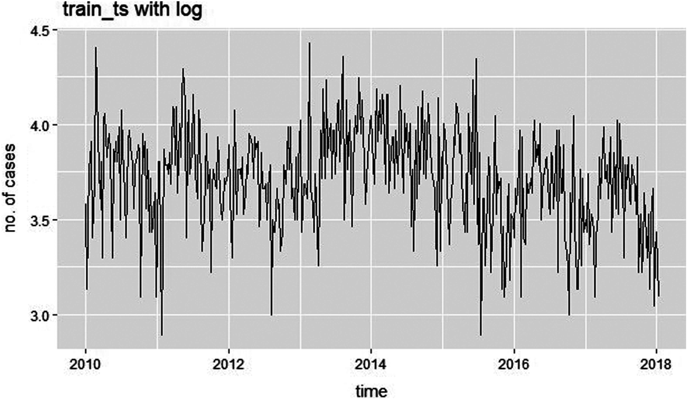
Figure 8: Time series plot on taking log of training data

In addition to this, the mentioned forecasting model is enforced on the time series as illustrated in Fig. 8 which is log⁡(train_ts) object. So, obtained fitted and forecasted plots are shown below in Figs. 9, 10, 11, 12, 13 and 14.

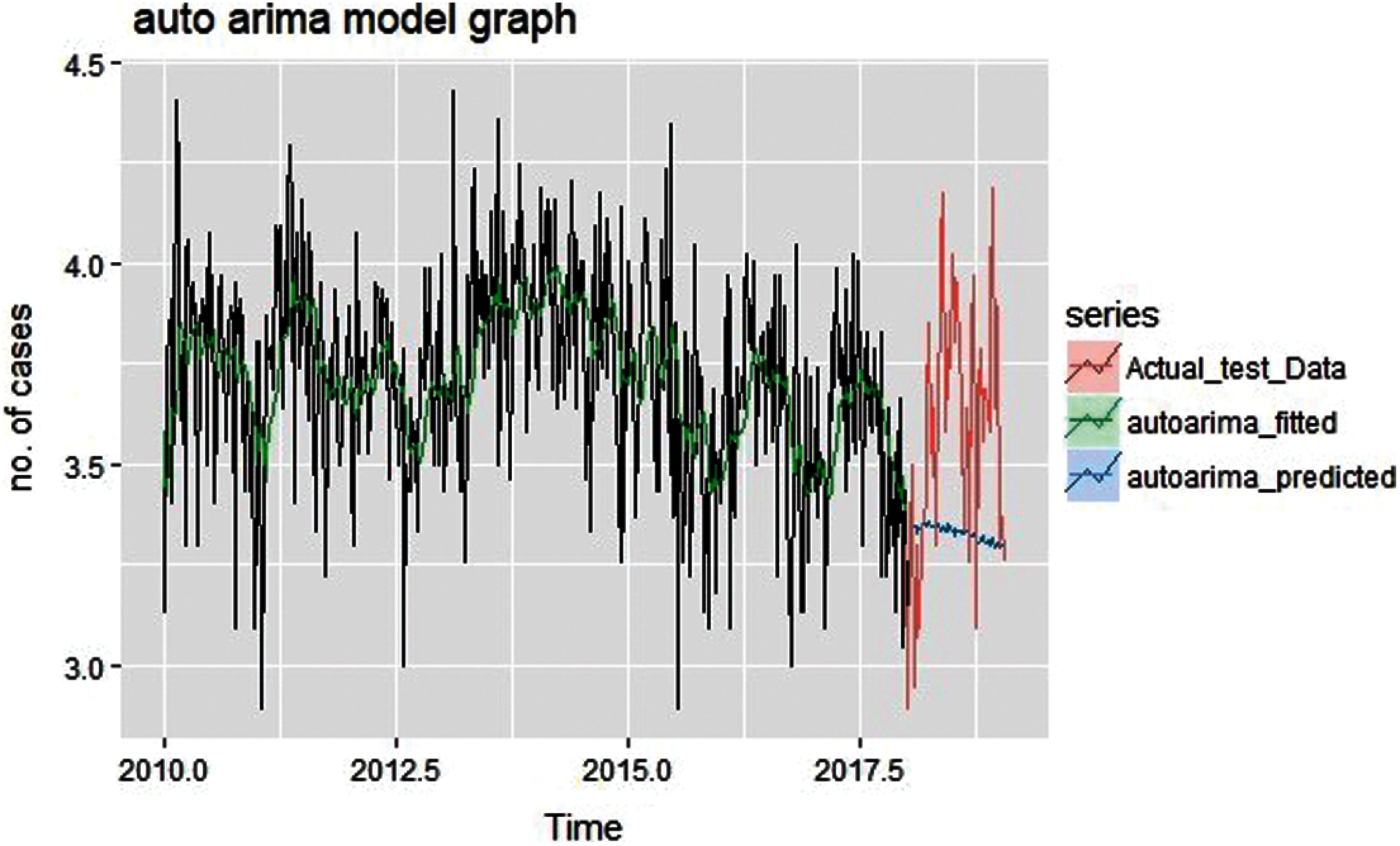
Figure 9: Fit values and forecast values of auto arima

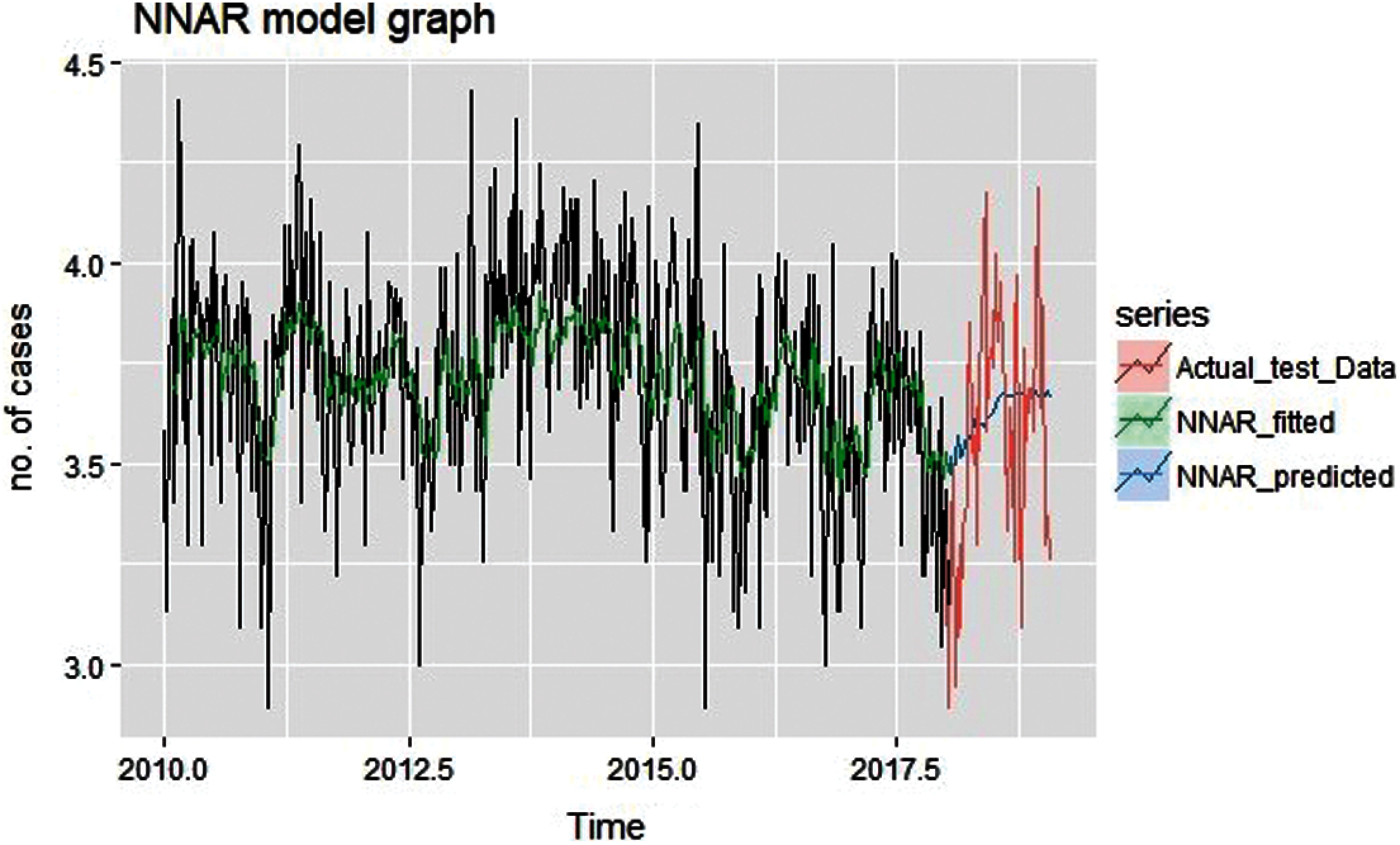
Figure 10: Fitted and predicted graph of NNAR

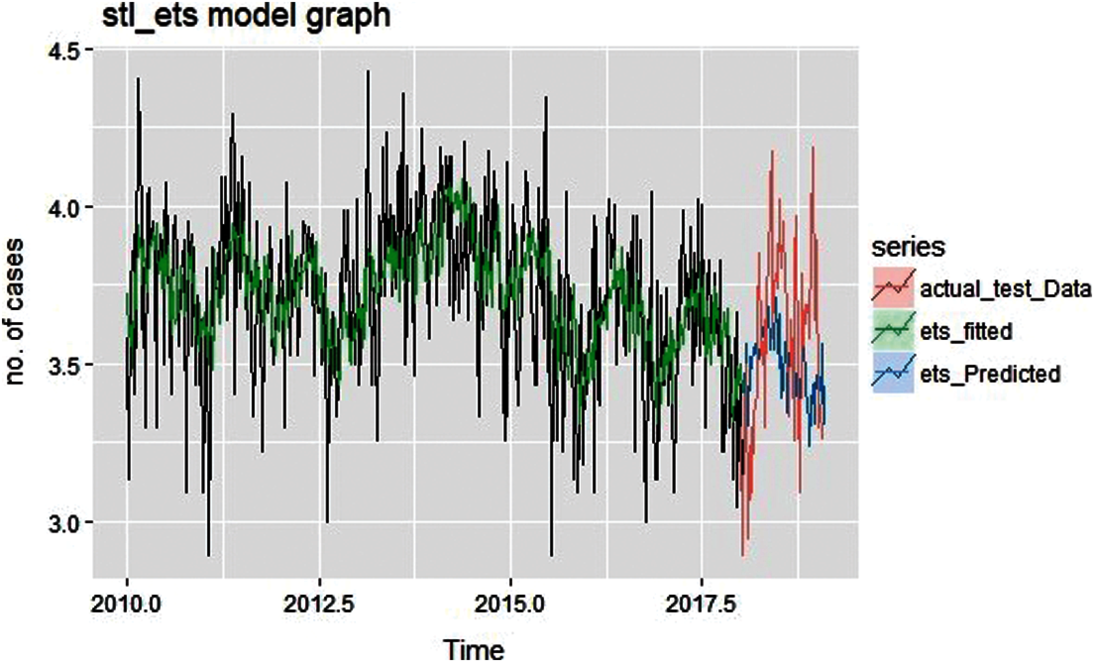
Figure 11: Fitted and predicted graph of ETS

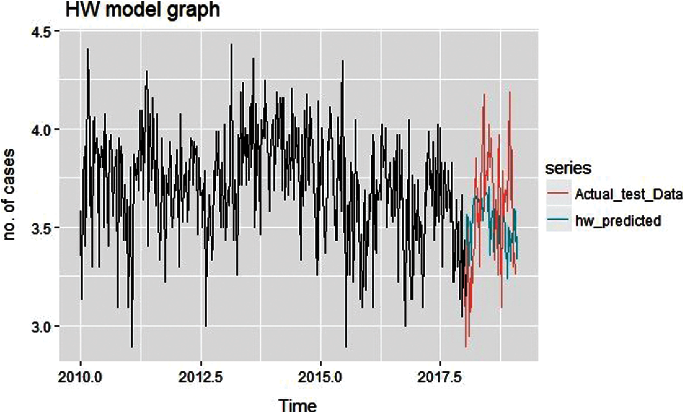
Figure 12: Predicted graph of Holt Winter

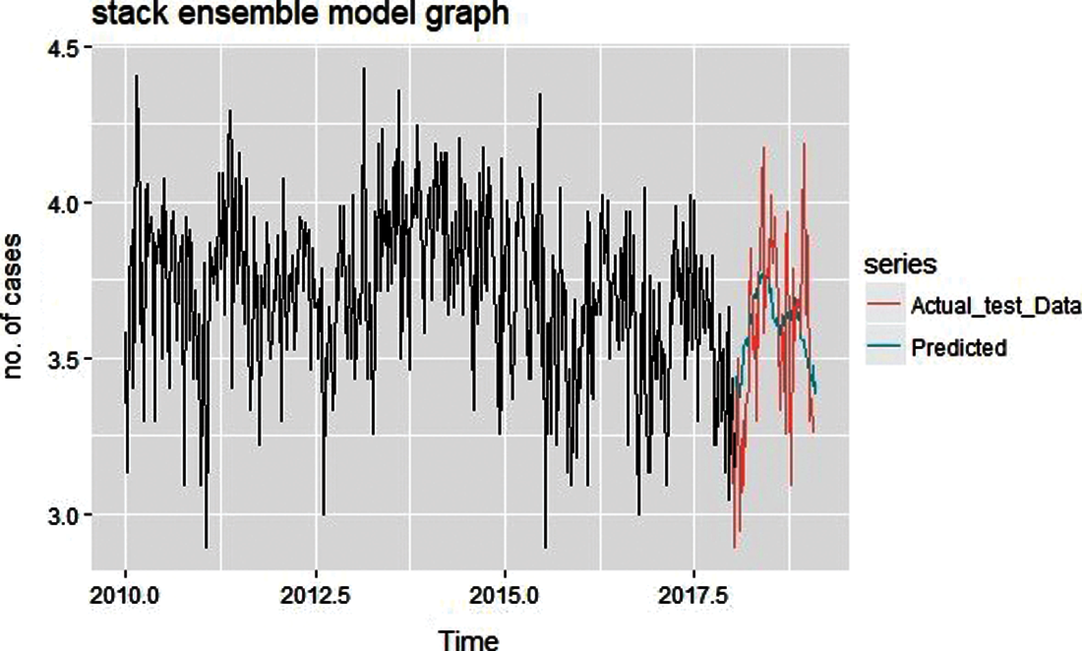
Figure 13: Predicted graph of stack generalization ensemble model

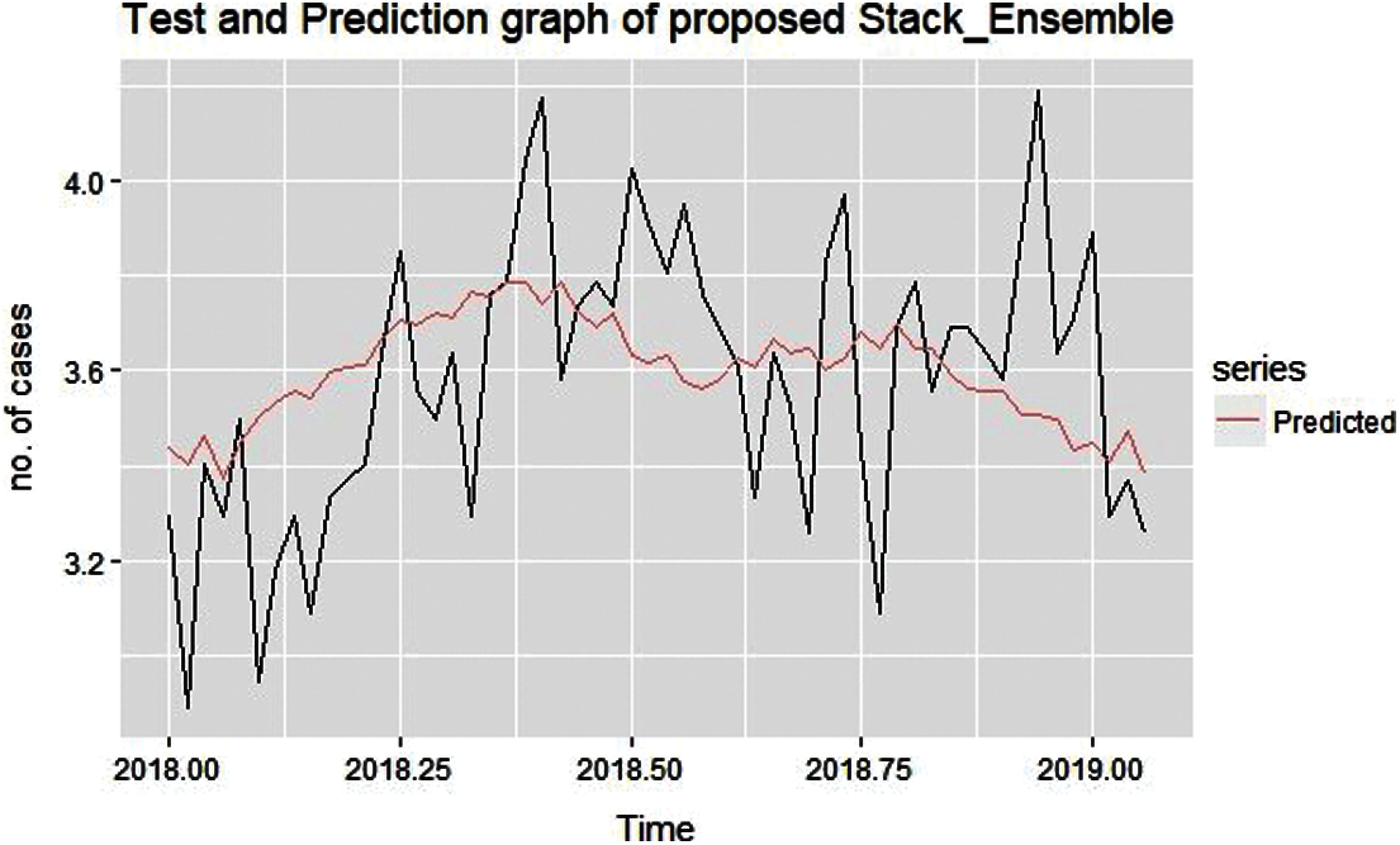
Figure 14: Predicted and test graph from stack ensemble model

Fig. 9 shows the fit values and forecast values obtained after the application of auto-Arima model, ARIMA(1,1,2)(1,0,0) on the training data, the forecasted values obtained in the graph reveals high difference in actual and predicted value.

Autoregressive neural network forecasted and fitted graph on actual training data shown in Fig. 10 describes that the forecasted graph doesn't have a similar trend as actual test dataset. This NNAR result obtains with neural network hyperparameter tuning and tuned parameter are as: set.seed(1234), and parameter P of nnetar() function is set to zero.

Fig. 11 shows fitted and predicted graph of ETS (Exponential Smoothing) with seasonality factor on actual training data, this shows that predicted graph is trying to follow the similar trend as test data but still there is too much diversity in results.

Holt Winter predicted graph on actual training data is shown in Fig. 12, here the predicted graph looks more promising and the result shows that it is better than the ETS and auto-Arima.

Proposed Ensemble model prediction graph for conjunctivitis disease for the year 2018–2019 is shown above in Figs. 13 and 14. Here used training data is the mean of the fitted values of three base models named as NAR, ETS and auto-arima.

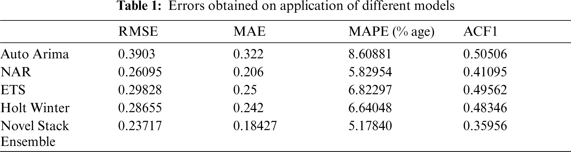
From the graph depicted in Figs. 13 and 14, it can be visualized that proposed stack ensemble model's predicted graph approximately follows a similar trend as test data set. So, predicted data is much closure to the actual number of cases of conjunctivitis for the period of January 2018 to December 2019. Different error metric from the ensemble model also decreases in comparison to the standard model. Tab. 1 depicts the error values obtained after applying the proposed ensemble model.

5  Conclusion

The main purpose of this research work is to present a novel forecasting model for conjunctivitis disease prediction. In this manuscript for conjunctivitis historical data from period 2010 to 2019, the available forecasting model are applied, then design a novel stack ensemble model by the combination of the used models in which three model used as the base model and one model is used as meta model of stack ensemble. The fitted value of all three base model given as training data to meta model then prediction made by meta model. After that, the final model is selected based on the comparison of trend depicted and error values of each model.

Here on the comparison, it can be safely concluded that the proposed novel stack ensemble has better prediction trend and less errors like RMSE, MAE, MAPE, ACF1 of the proposed ensemble is decreased significantly. Considering the RMSE for instance, it is 0.23717 for ensemble model which is 39.23%, 9.12%, 20.48%, and 17.23% less in compare of auto-Arima, Neural Network Autoregression, Exponential Smoothing, and Holt Winter model respectively. Therefore, the proposed stack ensemble model adopted as an optimal model for conjunctivitis disease prediction with promising results than another model. In future, the model can be extended by including other contributing factors such as rain, humidity, wind, etc.

Acknowledgement: This research was supported by Taif University Researchers supporting Project number (TURSP-2020/254), Taif University, Taif, Saudi Arabia.

Funding Statement: The authors would like to express their gratitude to Taif University, Taif, Saudi Arabia for providing administrative and technical support. This work was supported by the Taif University Researchers supporting Project number (TURSP-2020/254).

Conflicts of Interest: The authors declare that they have no conflicts of interest to report regarding the present study.

References

 1.  P. J. Brockwell and R. A. Davis, “Stationary Processes,” in Introduction to time series and forecasting, Springer-Verlag, New York: Springer, pp. 45–78, 2002. [Online]. Available: http://home.iitj.ac.in/parmod/document/introduction%20time%20series.pdf.

 2.  S. Verma and N. Sharma, “Statistical models for predicting chikungunya incidences in India,” in Proc. First Int. Conf. on Secure Cyber Computing and Communication, ICSCCC, Jalandhar, India, pp. 139–42, 2018.

 3.   D. Lai, “Monitoring the SARS epidemic in China: A time series analysis,” Journal of Data Science, vol. 3, pp. 279–293, 2005, http://www.jds-online.com/files/JDS-229.pdf.

 4.  X. Shao, C. S. Kim and D. G. Kim, “Accurate multi-scale feature fusion CNN for time series classification in smart factory,” Computers, Materials and Continua, vol. 65, no. 1, pp. 543–561, 2020.

 5.  A. Singh, J. C. Mehta, D. Anand, P. Nath, B. Pandey et al., “An intelligent hybrid approach for hepatitis disease diagnosis: Combining enhanced k-means clustering and improved ensemble learning,” Expert System, vol. 38, no. 1, pp. e12526, 2021.

 6.  Y. Ren, L. Zhang and P. N. Suganthan, “Ensemble classification and regression-recent developments, applications and future directions,” IEEE Computer Intelligent Magazine, vol. 11, no. 1, pp. 41–53, 2016.

 7.  K. Shashvat, R. Basu R, A. P. Bhondekar and A. Kaur, “A weighted ensemble model for prediction of infectious diseases,” Current Pharmaceutical Biotechnology, vol. 20, no. 8, pp. 674–678, 2019.

 8.  M. A. Khan, W. U. H. Abidi, M. A. Al Ghamdi, S. H. Almotiri, S. Saqib et al., “Forecast the influenza pandemic using machine learning,” Computers, Materials & Continua, vol. 66, no. 1, pp. 331–340, 2021.

 9.  B. Zhai and J. Chen, “Development of a stacked ensemble model for forecasting and analyzing daily average PM2. 5 concentrations in Beijing, China,” Science of the Total Environment, vol. 635, pp. 644–58, 2018.

10. J. Tamuli, A. Jain, A. V. Dhan, A. Bhan and M. K. Dutta, “An image processing based method to identify and grade conjunctivitis infected eye according to its types and intensity,” in Eighth Int. Conf. on Contemporary Computing (IC3), Noida, India, pp. 88–92, 2015.

11. H. Guo, S. Zhang, Z. Zhang, J. Zhang, C. Wang et al., “Short-term exposure to nitrogen dioxide and outpatient visits for cause-specific conjunctivitis: A time-series study in jinan, China,”Atmospheric Environment, vol. 247, pp. 118211, 2021.

12. H. Mpairwe, G. Nkurunungi, P. Tumwesige, H. Akurut, M. Namutebi et al., “Risk factors associated with rhinitis, allergic conjunctivitis and eczema among schoolchildren in Uganda,” Clinical & Experimental Allergy, vol. 51, no. 1, pp. 108–119, 2021.

13. N. Sultana and N. Sharma, “Statistical models for predicting swine f1u incidences in India,” in Proc. First Int. Conf. on Secure Cyber Computing and Communication (ICSCCC), Jalandhar, India, pp. 134–138, 2018.

14. S. M. Alotaibi, M. I. Basheer and M. A. Khan, “Ensemble machine learning based identification of pediatric epilepsy,” Computers, Materials and Continua, vol. 68, no. 1, pp. 149–165, 2021.

15. A. A. Ghorbani and K. Owrangh, “Stacked generalization in neural networks: Generalization on statistically neutral problems,” in Proc. Int. Joint Conf. on Neural Networks. Proc. (Cat. No.01CH37222), Washington, DC, USA, vol. 3, pp. 1715–1720, 2001.

16. K. W. Wang, C. Deng, J. P. Li, Y. Y. Zhang, X. Y. Li et al., “Hybrid methodology for tuberculosis incidence time-series forecasting based on ARIMA and NAR neural network,” Epidemiology & Infection, vol. 145, no. 6, pp. 1118–29, 2017.

17. N. Sultana, N. Sharma, K. P. Sharma, S. Verma, “A sequential ensemble model for communicable disease forecasting,” Current Bioinformatics, vol. 15, no. 4, pp. 309–317, 2020.

18. Conjunctivitis data: Hong Kong. Centre for Health Protection (CHP) of the Department of Health Hong Kong. 2019 [cited 2019 Mar 10]. Available: https://www.chp.gov.hk/en/index.html.

19. K. Shashvat, R. Basu, A. P. Bhondekar, S. Lamba, K. Verma et al., “Comparison of time series models predicting trends in typhoid cases in northern India,” Southeast Asian Journal of Tropical Medicine and Public Health, vol. 50, no. 2, pp. 347–56, 2019.

20. N. Sharma, J. Dev, M. Mangla, V. M. Wadhwa, S. N. Mohanty et al., “A heterogeneous ensemble forecasting model for disease prediction,” New Generation Computing, vol. 1, pp. 1–15, 2021.

21. P. Kumar and R. S. Thakur, “An approach using fuzzy sets and boosting techniques to predict liver disease,"Computers, Materials & Continua, vol. 68, no. 3, pp. 3513–3529, 2021.

This work is licensed under a Creative Commons Attribution 4.0 International License, which permits unrestricted use, distribution, and reproduction in any medium, provided the original work is properly cited.