DOI:10.32604/cmc.2022.021666
| Computers, Materials & Continua DOI:10.32604/cmc.2022.021666 | |
| Article |
Robust Length of Stay Prediction Model for Indoor Patients
1Department of Mechatronics and Control Engineering, University of Engineering and Technology, Lahore, 54000, Pakistan
2Department of Information Sciences, Division of Science and Technology, University of Education, Lahore, 54000, Pakistan
3Department of Computer Science and Information, College of Science in Zulfi, Majmaah University, Al-Majmaah, 11952, Saudi Arabia
4Riphah School of Computing & Innovation, Faculty of Computing, Riphah International University, Lahore Campus, Lahore, 54000, Pakistan
5Pattern Recognition and Machine Learning Lab, Department of Software, Gachon University, Seongnam, 13557, Korea
*Corresponding Author: Muhammad Adnan Khan. Email: adnan@gachon.ac.kr
Received: 08 July 2021; Accepted: 09 August 2021
Abstract: Due to unforeseen climate change, complicated chronic diseases, and mutation of viruses’ hospital administration’s top challenge is to know about the Length of stay (LOS) of different diseased patients in the hospitals. Hospital management does not exactly know when the existing patient leaves the hospital; this information could be crucial for hospital management. It could allow them to take more patients for admission. As a result, hospitals face many problems managing available resources and new patients in getting entries for their prompt treatment. Therefore, a robust model needs to be designed to help hospital administration predict patients’ LOS to resolve these issues. For this purpose, a very large-sized data (more than 2.3 million patients’ data) related to New-York Hospitals patients and containing information about a wide range of diseases including Bone-Marrow, Tuberculosis, Intestinal Transplant, Mental illness, Leukaemia, Spinal cord injury, Trauma, Rehabilitation, Kidney and Alcoholic Patients, HIV Patients, Malignant Breast disorder, Asthma, Respiratory distress syndrome, etc. have been analyzed to predict the LOS. We selected six Machine learning (ML) models named: Multiple linear regression (MLR), Lasso regression (LR), Ridge regression (RR), Decision tree regression (DTR), Extreme gradient boosting regression (XGBR), and Random Forest regression (RFR). The selected models’ predictive performance was checked using R square and Mean square error (MSE) as the performance evaluation criteria. Our results revealed the superior predictive performance of the RFR model, both in terms of RS score (92%) and MSE score (5), among all selected models. By Exploratory data analysis (EDA), we conclude that maximum stay was between 0 to 5 days with the meantime of each patient 5.3 days and more than 50 years old patients spent more days in the hospital. Based on the average LOS, results revealed that the patients with diagnoses related to birth complications spent more days in the hospital than other diseases. This finding could help predict the future length of hospital stay of new patients, which will help the hospital administration estimate and manage their resources efficiently.
Keywords: Length of stay; machine learning; robust model; random forest regression
Like any organization’s success is based on the updated information for its smooth functioning, in the same way, hospital administration’s utmost desire is to have updated data about the admitted patients and their stay in the hospitals. Since emergency cases are increasing day by day worldwide due to climate change as of COVID-19 [1] and population, it has become a severe issue for the hospital administration to deal with many inflows of patients. Most of the time, hospital management does not know when the existing patient leaves the hospital; this information could be crucial for hospital management. It could allow them to take more patients for admission [2]. Since patients’ Length of stay (LOS) has always remained unpredictable due to complicated issues like a mutation of viruses, chronic diseases, etc., hospital administrations face many problems related to managing available resources and admitting or facilitating new patients [3]. Therefore, it is essential to design such models that could help hospital administration predict patients’ LOS.
Machine learning (ML) has been widely used to predict the future based on the past behavior of data. A variety of ML models have been used to predict the LOS of the patients, including unsupervised and supervised ML models [4,5]. In unsupervised and supervised ML, the model is trained on an unlabeled and labeled dataset, respectively [6]. However, the supervised ML framework is more appropriate for a regression task like the one we address in this study. Therefore, in this study, the following supervised ML models, i.e., Multiple linear regression (MLR), Lasso regression (LR), Ridge regression (RR), Decision tree regression (DTR), Extreme gradient boosting regression (XGBR), and Random forest regression (RFR) have been selected and compared to predict the LOS of different diseased patients.
In the past, different ML techniques have been used to predict hospital LOS. Patients' stay in the hospitals is expected to increase due to the increase in cardiovascular diseases and the population's ages. This problem affects the healthcare system, with hospitals facing decreased bed capacity, and as a result, the overall cost is increased. To address this issue, in [7], a total of 16,414 cardiac patients were selected for the analysis of prediction of LOS by using ML models (i.e., Support vector machine (SVM), Bayesian network (BN), Artificial neural network (ANN), and RFR). The researcher concluded that the RFR model outperformed others with the highest accuracy score of 0.80. Morton et al. used supervised ML techniques such as MLR, SVM, Multi-task learning (MTL), and RFR model to predict the short period and the long period of diabetic patients' LOS. After comparing the results, it was recommended that SVM was more effective in predicting short period patients’ stay [8]. Bacchi et al. pre-processed 313 patient data and applied different ML techniques like ANN, Natural language processing (NLP), and SVM to develop predictions about LOS and discharge information. Their study revealed the ANN technique’s effectiveness in predicting the LOS with the highest accuracy of 0.74 [9]. Patel et al. correlated the performance of various combinations of variables for predicting hospital mortality and diabetic patients’ LOS. They concluded that the best combination of variables for predicting LOS by LR model was age, race, insurance status, type of admission, PR-DRG, and severity-calculation [10].
Walczak et al. used ANN techniques (i.e., Backpropagation (BP), Radial-basis-function (RBF), and Fuzzy ARTMAP) for predicting illness level and hospital LOS of trauma patients. They found out that combinations of BP and fuzzy ARTMAP produced optimal results [11]. Yang et al. used data of 1080 burnt patients and applied SVM and Linear regression (LR) techniques to predict the LOS for three different stages: admission, acute, and post-treatment. The study concluded that SVM regression performed better than the other regression techniques for LOS predictions across different stages of burnt patients [12]. Another group selected 896 surgical patients and applied supervised ML models (i.e., Local Gaussian Regression (LGR), SVM, and RFR) to make predictions about the LOS [13]. For this purpose, they made two groups of patients: Urgent-operational (UO) and non-Urgent-operational (non-UO) and found that blood sugar for the UO group and blood pressure for the non-UO group were the most influential variables in predicting the LOS. Their findings also revealed that the RFR model was the most accurate ML technique for predicting the LOS. Finally, Liu et al. used the dataset of seventeen hospitals of northern California and applied mixture models of Linear regression (LR) and Logistic regression (LR) to predict the LOS in hospitals [14]. They showed that Laboratory acute psychological score (LAPS) and Comorbidity point score (COPS) helped boost models’ efficiency.
A comparative analysis of exciting techniques to predict the LOS has been shown in Tab. 1. It has been observed that most of the studies are limited to a small dataset of patients and focus on only one or two specific diseases to calculate the LOS [8–11,13].

For the general recommendations to the hospital administration, we have selected a large dataset,i.e., more than 2.3 million patients, and included a range of diseases including Heart Transplant, Lungs Transplant, Burt Patients, Bone Marrow Transplant, Mental illness diagnoses, Liver Transplant, Intestinal Transplant, Schizophrenia, Respiratory System Diagnosis, Acute Leukemia, Eating disorder, Bipolar disorder, Trauma, Spinal disorder & injuries, Rehabilitation, Kidney Patients, Alcoholic Patients, Dialysis Patients, Skin Patients, HIV Patients, Malignant Breast disorder, Asthma, Cardiac/Heart-Patient, Cancer, Illness Severity, Surgery, Accident Patients, Respiratory distress syndrome, Abnormal Patients, etc. Above data is related to New-York hospitals. It contains patients’ information such as duration of stay, gender, age, race, ethnicity, type of admission, discharge year, and some other essential variables. The main objectives of this study are to explore the dataset to find the hidden patterns of variables and apply different supervised ML models to identify a robust model to make future predictions of the hospital LOS of different diseased patients. In this study, we also calculate the feature importance score by RFR model to identify which features among all the features are relevant to the hospital length of stay.
The framework of the proposed study to predict the LOS of the patients is presented in Fig. 1. Below, we briefly explain the various stages of the proposed framework.

Figure 1: A framework of the proposed study
In this study, we have used Inpatient De-identified data from healthdata.gov, a website managed by the U.S. Department of Health & Human Services that maintains updated health and social care data in the United States [15]. The dataset contains more than 2.3 million patients with 34 variables, listed in Tab. 2, including cost, charges, gender, age, race, ethnicity, type of admission, discharge year, etc., recorded in the year 2017.
It is essential for data analysis that the used data be correct and complete because missing values in the data negatively affect the model’s performance. For this purpose, the data set used for this study was checked, and missing values were identified. It was noticed that among all the variables listed in Tab. 2, ten variables had missing values. Three out of these ten variables, i.e., payment topology 2, payment topology 3, and birth weight, had a higher count of missing values than the rest and were removed from the dataset. However, the remaining seven variables, i.e., hospital service area, hospital county, operating certificate number, permanent facility id, zip code, ARR severity of illness description, APR risk of mortality, had a relatively low count of missing values. Therefore, we kept these variables, but corresponding rows information was removed for further analysis.

3.3 Data Exploration and Visualization
Exploratory data analysis (EDA) was used to analyze the dataset and summarize the dataset’s main variables [16]. In this study, univariate and bivariate analyses were applied to the variables to check the relationship between independent variables and target variable (LOS). Before performing both analyses, the correlation between all the input variables and the target variable (LOS) was checked. Correlation is a significant statistical concept that is used to find the relationship between variables. It has a range of values between −1 and +1, where −1 indicates a negative correlation and +1 indicates a positive correlation while 0 means there is no correlation between the variables [17]. Tab. 2 shows the correlation between independent variables and LOS (target variable).
As we can see from Tab. 2, Facility Name, Ethnicity, CCS Diagnosis Code, Zip Code, Race, APR Risk of Mortality, and APR Severity of Illness Description negatively correlate with LOS. Discharge Year, Abortion Edit Indicator, Payment Typology 2, Payment Typology 3 and Birth Weight have 0 correlation with LOS. While all the remaining variables have a positive correlation with LOS. Total Costs, CCS Diagnoses Code and Total Charges have the highest correlation with LOS. Variables “Discharge Year” and “Abortion Edit Indicator” were removed from the dataset for further analysis because they do not correlate with the target variable (LOS).
Since LOS is the output variable, we kept this variable along the y-axis of the plots created for Data Visualization. For example, in the dataset, the LOS of a patient with more than four months’ stay was given as 120+. Since exact days are not given in the dataset, we replaced 120+ with 130 to avoid the error.
Univariate analysis (UA) was used to explore variables of the dataset{Park, 2015 #51}. UA summarizes each variables’ dataset and identifies the hidden patterns of the dataset. In this study, as we can see in Fig. 2, the univariate distribution plot of LOS is displayed in the form of a normalized histogram. The plot shows that LOS distribution is not symmetric; most of the patients stayed almost

Figure 2: Univariate distribution plot of length of stay
Next, we performed the bivariate analyses to check the relationship between independent and output variables (LOS) using bar graphs. We have displayed the bar graphs in Figs. 3a--3f of some variables (i.e., APR Severity of Illness, Age Group, Type of Admission, APR Risk of Mortality, CCS Diagnoses Description, Patient Disposition, Payment Typology 1) that have shown maximum variance in a predictor variable(LOS). For example, the average values of LOS based on APR severity of illness is shown in Fig. 3a. As shown in Fig. 3a, the highest average LOS belongs to the extreme group followed by the major. Fig. 3b shows the average LOS of the different ages group. On average, more than 50 years old patients spent more days in the hospital than the patients of age groups 30--49 years old and the rest of the age groups. Fig. 3c shows the average length of hospital stays based on the admission type. As we can see from Fig. 3c, patients who belong to the “urgent” category of admission spent the highest number of days on average, followed by emergency based.

Figure 3: (a) Average length of stay based on APR severity of illness. (b) Average length of stay based on different age groups. (c) Average length of stay based on admission type. (d) Length of stay vs. different APR risk of mortality. (e) Top 10 diagnoses with the longest length of stay. (f) Length of stay vs. different patient disposition. (g) Average length of stay based on different payment methods
In contrast, the patients who belong to the “not available” category of admission spent the minimum number of days in the hospital on average. The average LOS based on APR risk of mortality is shown in Fig. 3d. As Fig. 3d reveals, the highest LOS on average belongs to the extreme group, followed by other groups. Based on the average LOS, as shown in Fig. 3e, patients with diagnoses related to birth complications spent more days in hospital followed by other diseases. Fig. 3f shows the average LOS of Patient disposition. On average, the highest average LOS belongs to the medical cert long term care hospitals, followed by the other dispositions. The average LOS for different payment types is also shown in Fig. 3g. We conclude that based on the average LOS as demonstrated in Fig. 3g, “Department of Corrections” and “unknown” categories of this feature (Payment Typology 1) have maximum average LOS followed by other categories of this feature.
Feature selection is an essential part of building a good model. ML requires important variables for training the model. There were a total of 34 variables in the patient’s dataset. After cleaning the dataset and performing EDA, some variables were removed due to a high count of missing values. The EDA helped gain further insights into the data. We used the Mutual Information (MI) regression technique to check the mutual dependence of input variables on the dependant variable (LOS). Information gain of all independent variables is shown in Fig. 4. Based on the EDA, ML models were trained using all the dataset’s variables (other than five variables removed due to the high count of missing values and zero correlation with the output variable (LOS).

Figure 4: Information gain of all independent variables based on LOS (i.e., predictor variable)
3.5 Machine Learning Regression Techniques
In this study, since the dataset is taken from the medical hospitals has an output in the form of a continuous numerical value; therefore, supervised ML regression algorithms were used to make predictions of the patient’s LOS. The chosen ML algorithms in this study are MLR, LR, RR, DTR, XGBR, and RFR, respectively.
3.5.1 Multiple Linear Regression Model
The multiple Linear Regression (MLR) model is an extension of Linear Regression (LR) which predicts a numeric value using more than one independent variable [18]. The general equation of the MLR model is:
where “y” is the output variable, “x” is the input variable and β is a constant term also named least square estimators.
Lasso regression (LR) model is a subtype of the linear regression model used to shrink the number of coefficients of the regression model. LR model is also used as a regularized regression model, which results in a sparse model with fewer coefficients. It makes some of the coefficients equal to zero, which are not contributing much to the predictions. As a result, the model becomes simpler, which performs better than the unregularized MLR model [19]. LR helps in reducing the overfitting problem by making the coefficients equal to zero for the least important features and keeping only those features that contribute to the output predictions.
Ridge regression (RR) is another particular case of linear regression model that helps shrink the coefficients and reducing the model’s complexity. It also helps in reducing multicollinearity. Unlike the LR model, the RR model does not provide absolute shrinkage of the coefficients. However, the RR model makes some of the coefficient values very low or close to zero. Therefore, the features which are not contributing much to the model will have very low coefficients. As a result, the RR model helps in reduces overfitting, which appears from the MLR model [20].
3.5.4 Decision Tree Regression Model and Extreme Gradient Boosting Regression Model
Decision tree regression (DTR) is a famous ML model used for classification and regression problems. DTR builds a tree-shaped structure of variables. DTR model breaks the data into smaller subsets, and the associated decision tree is incrementally developed simultaneously [21]. DTR model can handle both the numeric as well as categorical nature of data [22]. Extreme gradient boosting regression (XGBR) model is DTR based ensemble ML model [23]. This model is used to increase the speed and performance accuracy of the model.
3.5.5 Random Forest Regression Model
Random forest regression (RFR) model is a collection of multiple decision trees. RFR model is an estimator that fits several classifying decisions on the subsamples of the data and uses averaging criteria to improve the accuracy and control overfitting problems [24]. In the case of a classification problem, RFR uses voting criteria. Each tree in the RFR makes its prediction, and at the end, a class is assigned to a new test point based on the maximum voting. In the case of regression, it takes an average of all the numeric values predicted by the individual decision trees. In this way, it improves the accuracy and controls the overfitting of a model [25].
3.6 Model Evaluation and Validation
For parameter tuning, Cross-validation (CV) is a very useful technique used in ML modeling, and most of the time, it performs better than the standard validation set approach. It divides the data into k folds, e.g., 10-folds. Every time nine out of 10-folds go for training and the remaining one for testing. This process is repeated ten times so that all the folds go for training as well as for testing. In the end, average test accuracy is obtained [26]. One of the main advantages of CV over the simple validation set approach is that in CV, all the sample points go for training and testing, which is not the case in the simple validation set approach [27]. Fig. 5 shows the working of a K-fold CV. As we can see in Fig. 5, all the folds of the model are used for training and testing phases.
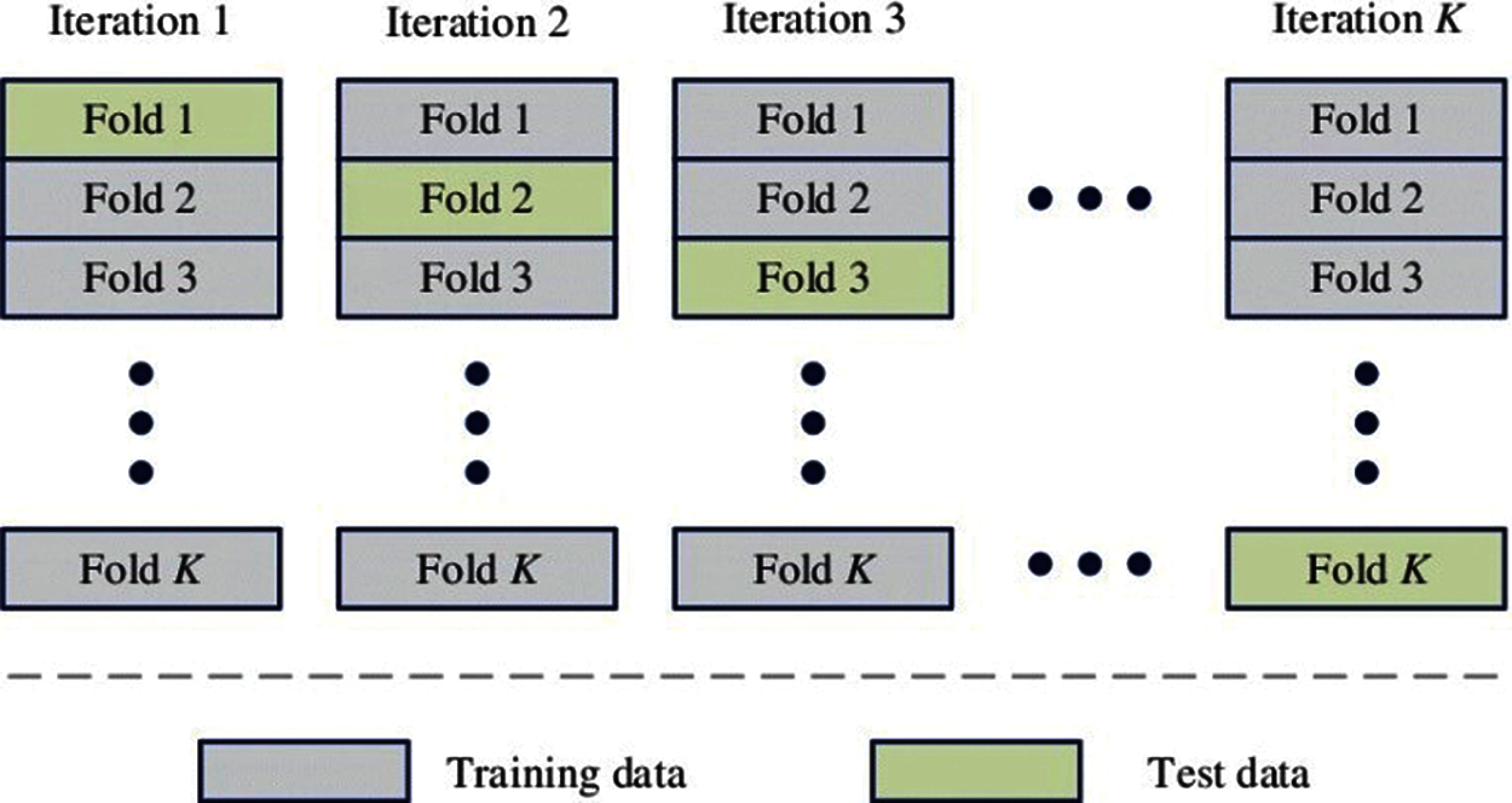
Figure 5: Working of K-fold cross-validation
After fitting the models, the next step is to measure the performances of the models. Two important performance measuring techniques, i.e., Mean square error (MSE) and R-square score, are used to measure the above-mentioned models’ performance. First, MSE is calculated by subtracting each predicted value from the actual value, then taking the square of each value and, in the end, adding all the squared values and dividing it by the number of training points. The following equation gives the mathematical formula for calculating MSE:
Here n denotes the number of training points, yi denotes the actual value, and ŷ denotes the value predicted by a model.
The second performance measurement technique is the R-square score, also known as the coefficient of determination. R-square has a value between 0 and 1. RS tells us how well a line fits the data or how well a line follows the variations within a set of data [28]. Mathematically it is given as:
SSRES denotes the sum of squares of residuals, and SSTOT denotes the sum of squares of the total. R-square value of 1 indicates a perfectly best-fitted model, while a score of 0 says the model was unable to fit the data and it is a poorly fitted model.
After selecting essential variables of the dataset, six selected models, i.e., MLR, LR, RR, DTR, XGBR, and RFR, were evaluated using a 10-fold CV. For this purpose, the dataset was divided into an 80:20 ratio, i.e., 80% for the training and 20% for testing. The train data with a similar proportion was separated for the training and validation portion. The main idea is to train and validate the model first using 10 folds’ CV for parameter tuning and then testing the model on 20% of the test data to see the model’s performance on the test predictions. For the 10-fold CV, the model was built ten times on nine different folds, validated on the tenth fold. In the end, the mean value was taken off ten folds for R-square and MSE. R-square tells us how best the model fits the data, and MSE is the cost function of MLR, which is the square root of the sum of the difference between the actual and predicted value of each record. In the case of best model performance, the MSE result should be minimum (0 in perfect conditions), and the R-square score should be near or equal to 1. The parameter settings corresponding to the minimum validation average were selected for prediction in the test phase.
4.1.1 Multiple Linear Regression Model
Multiple linear regression (MLR), as mentioned before, was trained and validated using a 10-fold CV for the prediction of LOS. Then MLR model was used to predict the x-test to see its performance on the test-data. MSE on the training data was 39, and the R-square score of the training data was 0.37. So, both MSE and R-square results showed that the MLR model’s performance was very low on the training data. And on the test data showed an MSE of 38.49, and the R-square score was 0.371. So in the case of both training and testing, MSE was very high, and the R-square score was very low, which indicated a low performance of the MLR model.
Lasso regression (LR) model was applied in a way very similar to the MLR model. LR model showed an MSE of 42.58 and an R-square score of 0.31 for the training data. For the test data, the LR model showed an MSE of 42.19 and an R-square score of 0.310. Thus, for both cases (training and testing), MSE was even higher than MLR, and the R-square score was very low, resulting in low model performance.
The Ridge regression (RR) model showed an MSE of 39 and an R-square score of 0.37 for the training data. However, it showed an MSE of 38.49, and the R-square score was 0.3711 for the test data. Since these results were also far from ideal, RR model performance was also low.
4.1.4 Decision Tree Regression Model
The Decision tree regression (DTR) Model showed an MSE of 0.002 and an R-square score of 0.999 for the training data. However, it showed an MSE of 5.93, and the R-square score was 0.903 for the test data. Since these results were relatively close to the ideal, this model's performance was much better than MLR, LR, and RR.
4.1.5 Extreme Gradient Boosting Regression Models
The Extreme gradient boosting regression (XGBR) model showed an MSE of 5.32 and an R-square score of 0.914 for the training data. However, it showed an MSE of 5.62, and the R-square score was 0.908 for the test data. As the readings indicate, XGBR performed better than all the previous models.
4.1.6 Random Forest Regression Model
Random forest regression (RFR) model was also applied in the same way as other models. RFR model showed an MSE of 0.76 and an R-square score of 0.987 for the training data. However, it showed an MSE of 5 and an R-square score of 0.92 for the test data. These results indicate the superior predictive performance of the RFR method as compared to other models.
We have seen that MLR, LR, and RR models could not perform well, as indicated by large MSE and small R-square scores. However, the other two models, i.e., DTR and XGBR, were better in terms of these performance measures, as presented in Tab. 3. Thus, overall, the RFR model was found the best model to predict the LOS.
From Tab. 3, it can be seen that both in terms of R-square score and MSE score, the RFR model is the best one, followed by the XGBR model. RFR was the model in which explanatory variables explained the variation in y output variable (LOS) with the highest R-square score of 92% and the lowest MSE score of 5 among all six models. XGBR ensemble algorithm is the second-best model in this analysis, with an R-square score of 90.8% and an MSE score of 5.62. MLR, RR, and LR could not fit this hospital data properly and performed poorly on the data. This proposed methodology outperformed with a large dataset and achieved a higher accuracy rate than other studies done in the past.

Features importance is an important technique used to identify which features/variables among all the features/variables are relevant in making predictions. Feature prediction scores were calculated using the RFR model [29]. Feature’s importance tells which features primarily contribute to fitting the data or explaining the variation/prediction of the output variable y [30]. It can be seen in Fig. 6 that “Total Costs”, “CCS Diagnosis”, and “Total Charges” are the essential variables in terms of the importance score. These results are consistent EDA findings, where LOS was found to have a high correlation score with these variables. Apart from these three variables, Fig. 6 also reveals the part played by other variables, although secondary, in predicting the LOS.
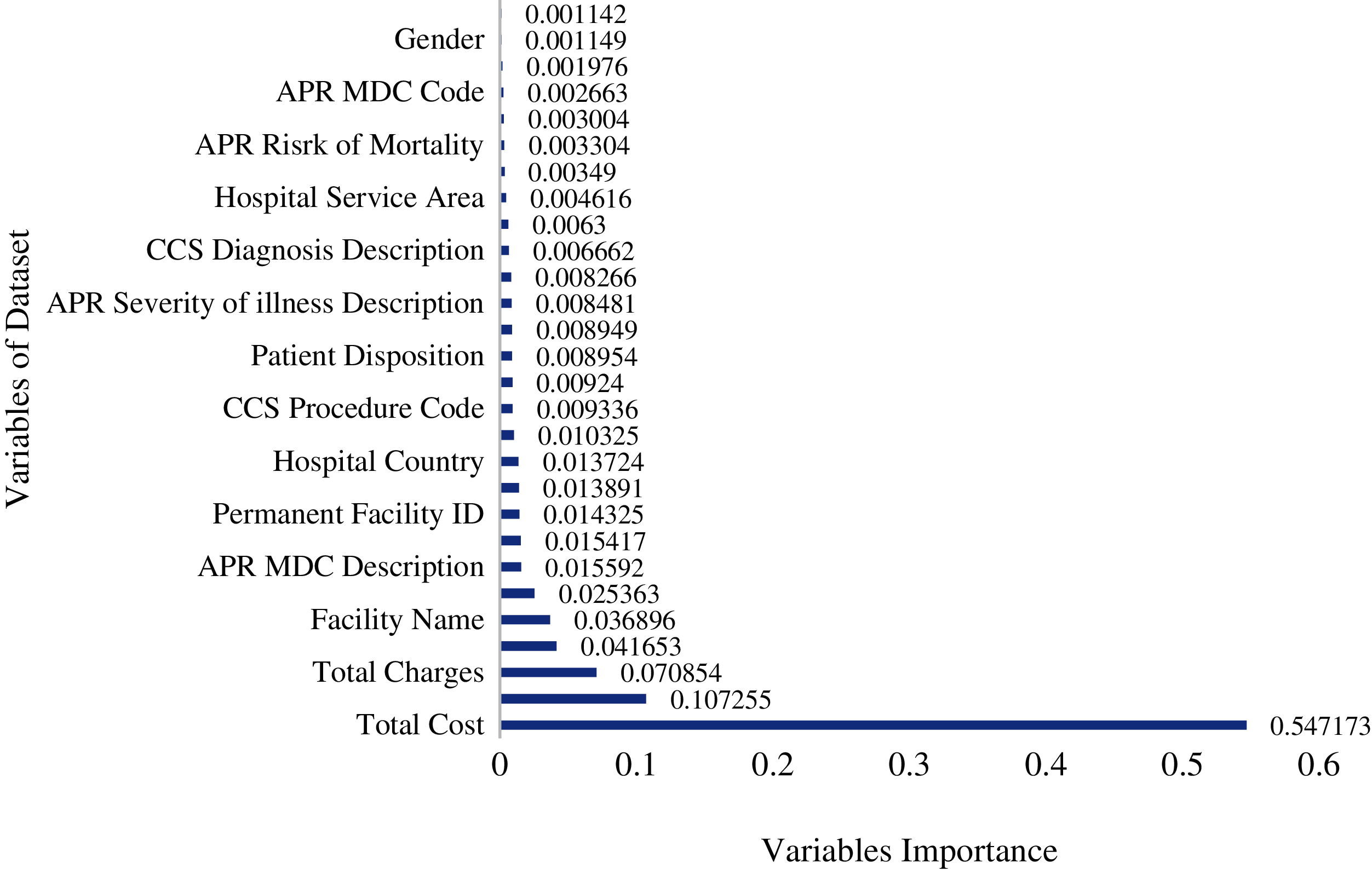
Figure 6: Importance of independent variables on length of stay in random forest model
In this study, the main objectives were to explore the Inpatient De-identified data and to build a robust model that could predict the hospital LOS of patients coming to the hospital in the future. Predicting hospital length of stay will help hospitals estimate resources available for the patients and manage the available resources efficiently. EDA with the help of graphs was performed to develop essential insights from the data. By EDA, we conclude that maximum stay was between 0 to 5 days with the meantime of each patient 5.3 days and more than 50 years old patients spent more days in the hospital. Based on the average LOS, it was also observed that the patients with diagnoses related to birth complications spent more days in the hospital than other diseases. Six ML models were employed and evaluated by using the 10-fold CV approach. Linear multiple regression (LMR), Lasso regression (LR), Ridge regression (RR), Decision tree regression (DTR), Extreme gradient boosting regression (XGBR), and Random forest regression (RFR) were the chosen models in this analysis. The results showed that RFR was the best model for R-square and MSE, followed by the XGBR. Feature importance score revealed the relevance of three primary variables, Total Costs, CCS Diagnoses Code, and Total Charges, for predicting the LOS. Based on the above-detailed study, we recommend that future work involve more variables in the given dataset to build a more accurate model that could predict hospital LOS more accurately.
Acknowledgement: Thanks to the supervisor and co-authors for their valuable guidance and support.
Funding Statement: The authors received no specific funding for this study.
Conflicts of Interest: The authors declare that they have no conflicts of interest to report regarding the present study.
1. A. Gumaei, M. A. Rakhami, M. M. A. Rahhal, F. R. H. Albogamy, E. A. Maghayreh et al., “Prediction of COVID-19 confirmed cases using gradient boosting regression method,” Computers, Materials & Continua, vol. 66, no. 1, pp. 315–329, 2020. [Google Scholar]
2. R. Mitchell and C. Banks, “Emergency departments and the COVID-19 pandemic: Making the most of limited resources,” Emergency Medicine Journal, vol. 37, no. 5, pp. 258–259, 2020. [Google Scholar]
3. H. M. Zolbanin, B. Davazdahemami, D. Delen and A. H. Zadeh, “Data analytics for the sustainable use of resources in hospitals: Predicting the length of stay for patients with chronic diseases,” Information & Management, vol. 13, no. 4, pp. 103282–103299, 2020. [Google Scholar]
4. M. T. Chuang, Y. H. Hu and C. L. Lo, “Predicting the prolonged length of stay of general surgery patients: A supervised learning approach,” International Transactions in Operational Research, vol. 25, no. 1, pp. 75–90, 2018. [Google Scholar]
5. S. Uddin, A. Khan, M. E. Hossain and M. A. Moni, “Comparing different supervised machine learning algorithms for disease prediction,” BMC Medical Informatics and Decision Making, vol. 19, no. 1, pp. 1–16, 2019. [Google Scholar]
6. B. C. Love, “Comparing supervised and unsupervised category learning,” Psychonomic Bulletin & Review, vol. 9, no. 4, pp. 829–835, 2002. [Google Scholar]
7. T. A. Daghistani, R. Elshawi, S. Sakr, A. M. Ahmed, A. A. Thwayee et al., “Predictors of in-hospital length of stay among cardiac patients: A machine learning approach,” International Journal of Cardiology, vol. 288, pp. 140–147, 2019. [Google Scholar]
8. A. Morton, E. Marzban, G. Giannoulis, A. Patel, R. Aparasu et al., “A comparison of supervised machine learning techniques for predicting short-term in-hospital length of stay among diabetic patients,” in Int. Conf. on Machine Learning and Applications, Detroit, MI, USA, pp. 1–5, 2014. [Google Scholar]
9. S. Bacchi, S. Gluck, Y. Tan, I. Chim, J. Cheng et al., “Prediction of general medical admission length of stay with natural language processing and deep learning: A pilot study,” Internal and Emergency Medicine, vol. 15, no. 6, pp. 989–995, 2020. [Google Scholar]
10. A. Patel, M. Johnson and R. Aparasu, “Predicting in-hospital mortality and hospital length of stay in diabetic patients,” Value in Health, vol. 16, no. 3, pp. A17–A25, 2013. [Google Scholar]
11. M. W. Nadeem, M. A. A. Ghamdi, M. Hussain, M. A. Khan, K. M. Khalid et al., “Brain tumor analysis empowered with deep learning: A review, taxonomy, and future challenges,” Brain Sciences, vol. 10, no. 2, pp. 118–134, 2020. [Google Scholar]
12. C. S. Yang, C. P. Wei, C. C. Yuan and J. Y. Schoung, “Predicting the length of hospital stay of burn patients: Comparisons of prediction accuracy among different clinical stages,” Decision Support Systems, vol. 50, no. 1, pp. 325–335, 2010. [Google Scholar]
13. M. T. Chuang, Y. H. Hu and C. L. Lo, “Predicting the prolonged length of stay of general surgery patients: a supervised learning approach,” International Transactions in Operational Research, vol. 25, no. 1, pp. 75–90, 2018. [Google Scholar]
14. V. Liu, P. Kipnis, M. K. Gould and G. J. Escobar, “Length of stay predictions: Improvements through the use of automated laboratory and comorbidity variables,” Medical Care, vol. 48, no. 8, pp. 739–744, 2010. [Google Scholar]
15. SPARCE, “Hospital inpatient discharges (SPARCS De-Identified). State of New York, 2017. [Online]. Available: https://healthdata.gov/dataset/hospital-inpatient-discharges-sparcs-de-identified. [Google Scholar]
16. M. L. Vigni, C. Durante and M. Cocchi, “Exploratory data analysis,” Data Handling in Science and Technology, vol. 28, pp. 55–126, 2013. [Google Scholar]
17. S. Kumar and I. Chong, “Correlation analysis to identify the effective data in machine learning: Prediction of depressive disorder and emotion states,” Environmental Research and Public Health, vol. 15, no. 12, pp. 2907, 2018. [Google Scholar]
18. T. Catalina, V. Iordache and B. Caracaleanu, “Multiple regression model for fast prediction of the heating energy demand,” Energy and Buildings, vol. 57, no. September (9), pp. 302–312, 2013. [Google Scholar]
19. F. E. Streib and M. Dehmer, “High-dimensional LASSO-based computational regression models: regularization, shrinkage, and selection,” Machine Learning and Knowledge Extraction, vol. 1, no. 1, pp. 359–383, 2019. [Google Scholar]
20. B. G. Kibria and A. M. E. Saleh, “Improving the estimators of the parameters of a probit regression model: A ridge regression approach,” Journal of Statistical Planning and Inference, vol. 142, no. 6, pp. 1421–1435, 2012. [Google Scholar]
21. W. Y. Loh, “Classification and regression tree methods,” in Encyclopedia of Statistics in Quality and Reliability, University of Wisconsin, Madison, Wisconsin, vol. 1, pp. 315–323, 2008. [Google Scholar]
22. M. Xu, P. Watanachaturaporn, P. K. Varshney and M. K. Arora, “Decision tree regression for soft classification of remote sensing data,” Remote Sensing of Environment, vol. 97, no. 3, pp. 322–336, 2005. [Google Scholar]
23. J. Liu, J. Wu, S. Liu, M. Li, K. Hu et al., “Predicting mortality of patients with acute kidney injury in the ICU using XGBoost model,” PLoS One, vol. 16, no. 2, pp. e0246306, 2021. [Google Scholar]
24. D. S. Palmer, N. M. O. Boyle, R. C. Glen and J. B. Mitchell, “Random forest models to predict aqueous solubility,” Journal of Chemical Information and Modeling, vol. 47, no. 1, pp. 150–158, 2007. [Google Scholar]
25. A. Liaw and M. Wiener, “Classification and regression by random forest,” R News, vol. 2, no. 3, pp. 18–22, 2002. [Google Scholar]
26. M. W. Browne, “Cross-validation methods,” Journal of Mathematical Psychology, vol. 44, no. 1, pp. 108–132, 2000. [Google Scholar]
27. C. Bergmeir, M. Costantini and J. M. Benítez, “On the usefulness of cross-validation for directional forecast evaluation,” Computational Statistics & Data Analysis, vol. 76, no. 7, pp. 132–143, 2014. [Google Scholar]
28. A. C. Cameron and F. A. G. Windmeijer, “An R-squared measure of goodness of fit for some common nonlinear regression models,” Journal of Econometrics, vol. 77, no. 2, pp. 329–342, 1997. [Google Scholar]
29. V. Sugumaran, V. Muralidharan and K. Ramachandran, “Feature selection using decision tree and classification through proximal support vector machine for fault diagnostics of roller bearing,” Mechanical Systems and Signal Processing, vol. 21, no. 2, pp. 930–942, 2007. [Google Scholar]
30. Y. Gupta, “Selection of important features and predicting wine quality using machine learning techniques,” Procedia Computer Science, vol. 125, no. 1, pp. 305–312, 2018. [Google Scholar]
 | This work is licensed under a Creative Commons Attribution 4.0 International License, which permits unrestricted use, distribution, and reproduction in any medium, provided the original work is properly cited. |