Computers, Materials & Continua DOI:10.32604/cmc.2022.021498
Article

Primary User-Awareness-Based Energy-Efficient Duty-Cycle Scheme in Cognitive Radio Networks

Zilong Jin1,2, Chengbo Zhang1, Kan Yao3, Dun Cao4, Seokhoon Kim5 and Yuanfeng Jin6,*

1School of Computer Science, Nanjing University of Information Science and Technology, Nanjing, 210044, China
2Jiangsu Collaborative Innovation Center of Atmospheric Environment and Equipment Technology (CICAEET) Nanjing University of Information Science and Technology, Nanjing, 210044, China
3Jiangsu Institute of Economic and Information Technology, Nanjing, 210003, China
4School of Computer and Communications Engineering, Changsha University of Science and Technology, Changsha, 410114, China
5Department of Computer Software Engineering, Soonchunhyang University, Asan, 31538, Rep. of Korea
6Department of Mathematics, Yanbian University, Yanji, 133002, China
*Corresponding Author: Yuanfeng Jin. Email: yfkim@ybu.edu.cn
Received: 05 July 2021; Accepted: 09 August 2021

Abstract: Cognitive radio devices can utilize the licensed channels in an opportunistic manner to solve the spectrum scarcity issue occurring in the unlicensed spectrum. However, these cognitive radio devices (secondary users) are greatly affected by the original users (primary users) of licensed channels. Cognitive users have to adjust operation parameters frequently to adapt to the dynamic network environment, which causes extra energy consumption. Energy consumption can be reduced by predicting the future activity of primary users. However, the traditional prediction-based algorithms require large historical data to achieve a satisfying precision accuracy which will consume a lot of time and memory space. Moreover, many of these schemes lack methods to deal with the very busy network environments. In this paper, one semi-supervised learning algorithm, i.e., tri-training, has been employed to investigate the prediction of primary activity. Based on the prediction results of tri-training, a duty-cycle mechanism and an intermediate node selection approach are proposed to improve the energy efficiency. Simulation results show the effectiveness of the proposed algorithm.

Keywords: Cognitive radio; tri-training; duty-cycle; intermediate node; energy efficiency

1  Introduction

Cognitive radio (CR) has been a promising technology to solve the spectrum crisis caused by the rapidly growing communication requirement in the Industrial Scientific Medical (ISM) band [1,2]. The key technology of CR is the dynamic spectrum access, which allows the cognitive radio-enabled devices i.e., Secondary Users (SUs) to utilize the licensed spectrum resource without interfering the Primary User (PU) to improve the spectrum efficiency [3–5].

However, PU's activity varies in temporal and spatial domain makes the data transmission of SUs is interrupted to prevent interference, which will cause unstable transmission [6,7]. Unstable transmission causes energy waste and load unbalanced [8–10] which is unacceptable in battery-powered cognitive radio networks (CRNs). Therefore, data transmission in cognitive radio networks should avoid the hot area of PU's activity.

In the transmission of multi-hop CRNs, available channels of SUs change from time to time and hop by hop [11–13]. If PU's activity is frequent, the SUs will have no common available channels with their neighbors, and it cannot transmit or be an intermediate node for any transmission. In this case, any attempt by a SU for transmission is a waste of energy consumption. Thus, SUs should be aware of the busy network environment and stop any redundant behavior to improve energy efficiency [14].

Related researches are presented to reduce energy consumption. Channel usage patterns prediction-based schemes are presented for transmission and mainly fall into Markovian model-based and statistics-based. In [15], basic HMM-based prediction methods were proposed to learn the traffic characteristics of the licensed channels. Hamid Eltom et al. proposed a hard-fusion-based spectrum occupancy prediction scheme to enhance the prediction accuracy [16]. However, these schemes cannot predict how long the PUs will occupancy the licensed channel. Instead of traditional Markovian models, Saad et al. introduced an HMM-based spectrum prediction that several time slots of the spectrum occupancy can be predicted [17]. However, each round of prediction needs a long duration of sampling to guarantee the prediction precision, and that is not applicable for memory-limited wireless equipment.

Monemian et al. [18] proposed a cooperative spectrum sensing scheme to optimize energy consumption. This method divides the SUs into several sensing clusters according to the local detection probability and the global detection probability. As long as the global detection accuracy is satisfied, SUs with a lower detection probability can be grouped into a group with SUs with a higher detection probability. Cooperative spectrum sensing is carried out by selecting the group with the smallest average energy consumption (including the energy consumption for spectrum sensing and transmission of sensing results), and sharing channel state decision information with other SUs, until all sensing clusters no longer meet the detection accuracy and energy idle. Akan [19] proposed a two-stage cooperative spectrum sensing method. The first stage performs fast coarse spectrum sensing to find possible available channels; in the second stage, a more accurate fine spectrum sensing scheme is used to make the final decision on the sensing results of the first stage. Ren et al. [20] improved energy efficiency by minimizing the number of SUs involved in spectrum sensing. At the same time, this solution further improves the energy efficiency of cooperative spectrum sensing by adaptively adjusting the number of SUs of spectrum sensing. The above schemes mostly use the current information of the nodes for sensing node selection or sensing channel decisions, etc., lacking effective knowledge of future network environment changes, and missing adjustments to spectrum sensing activities (such as stopping spectrum sensing for channels that may not be available) opportunities to improve energy efficiency.

Shamsad Parvin et al. presented a Channel Priority Lists (CPL) scheme for transmission in multi-hop CRNs [21]. In this scheme, the channel status is measured by the usage ratio of PUs. However, studies show that the spectrum occupancy peaks at about 14%, except under emergency conditions where occupancy can reach 100% for brief periods. The usage ratio is a global value, that cannot reflect the real-time spectrum status.

Meanwhile, a duty-cycled approach was designed by Amna Jamal et al. in [22]. In the duty-cycle mechanism, a SU goes to sleep for a predetermined time if no transmission requests from other SUs are received and the SU has no data to transmit. However, since the predetermined sleep time is stationary, thus this scheme cannot be applied in the CRNs in which the spectrum access is dynamically changed.

In this paper, one semi-supervised learning-based prediction scheme, i.e., tri-training [23], is employed to solve these problems, which combines a duty-cycle mechanism and an intermediate node selection approach. The main contributions can be summarized as follows:

(1)   A tri-training based learning algorithm is employed to reduce the number of historical data needed for prediction, thus the memory cost of the SU can be optimized. Meanwhile, considering the unreliable spectrum sensing results can be a noisy labeled example in training for prediction; the transmission results (which contain the intermediate node, channel for transmission, et al.) will be used as the training data but not spectrum sensing results.

(2)   A prediction-based intermediate node and channel selection scheme is proposed for transmission to improve the throughput. Meanwhile, the transmission results but not the spectrum sensing results are used as the training data to optimize the noise rate in the labeled example.

The rest of the paper is organized as follows. Section II describes the system model. The proposed tri-training based prediction scheme including duty-cycle approach, intermedia node and channel selection is presented in Section III. Section IV provides simulation results of the proposed scheme and Section V concludes the paper.

2  System Model & Problem Definition

2.1 Cognitive Radio Network Model

As shown in Fig. 1, a distributed multi-hop cognitive radio network, consisting of Npu PUs and Nsu SUs is considered. Let M be the total number of licensed channels. Each PU is allocated to one licensed channel (data channel), thus the number of data channels equals the number of PUs (Npu=M). A Common Control Channel (CCC) is devoted to transmitting and receiving control information (i.e., spectrum sensing results) between neighboring SUs. It is assumed that each SU is immobile and follows a sleep/active cycle. Upon active phase, SU performs spectrum sensing and listens to the CCC for transmission requests. Upon sleep phase, SUs will stop any behavior (spectrum sensing, et al.) to save energy.

Meanwhile, the structure of a frame is introduced as depicted in Fig. 2. Each frame consists of m time slots from τ1 to τm, each time slot contains spectrum sensing phase and transmission phase. For a frame, it has 2 states, active/sleep and the details will be described in the proposed scheme part.

2.2 Problem Definition

For example, as depicted in Fig. 1, the network consists of one sink node, eight SUs (from d1 to d8) and one PU, PU occupies its own licensed channel ch1. Since the sink node is not within the transmission range of d3, the data transmission between the sink and d3 requires d5 or d6 as an intermediate node (when the routing method is based on greedy algorithm). However, both of the nodes cannot be intermediate nodes while they are interfered with PU, since they have no common channel with neighboring SUs. In this case, the transmission path will avoid d5 and d6, and d1will be selected as the intermediate node. After d7 receiving the data, all licensed channels are unavailable, thus there is no need for d7 to perform spectrum sensing and data exchange, and it will enter a sleep mode to save energy in such a timeframe.

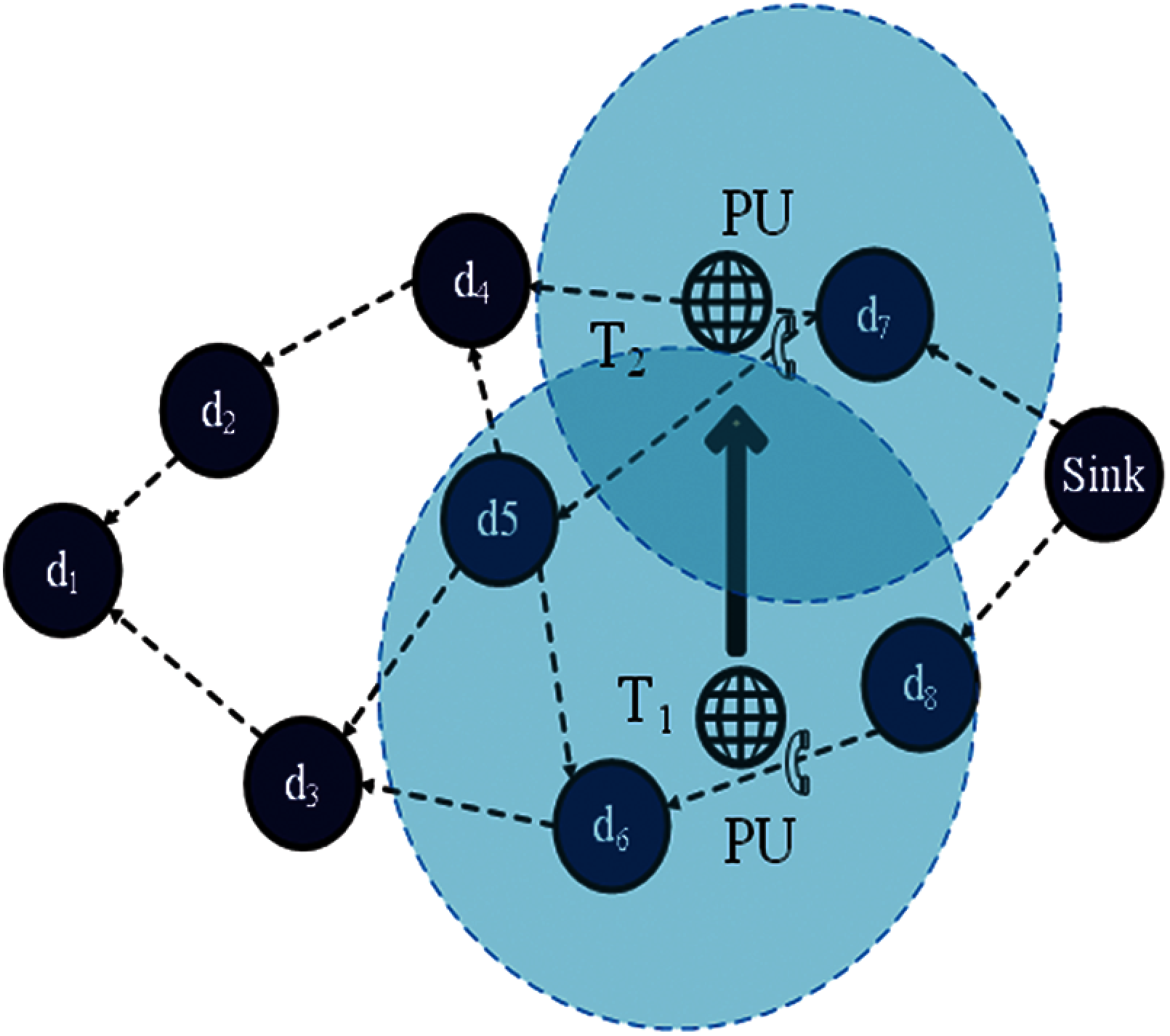
Figure 1: A model of the cognitive radio network

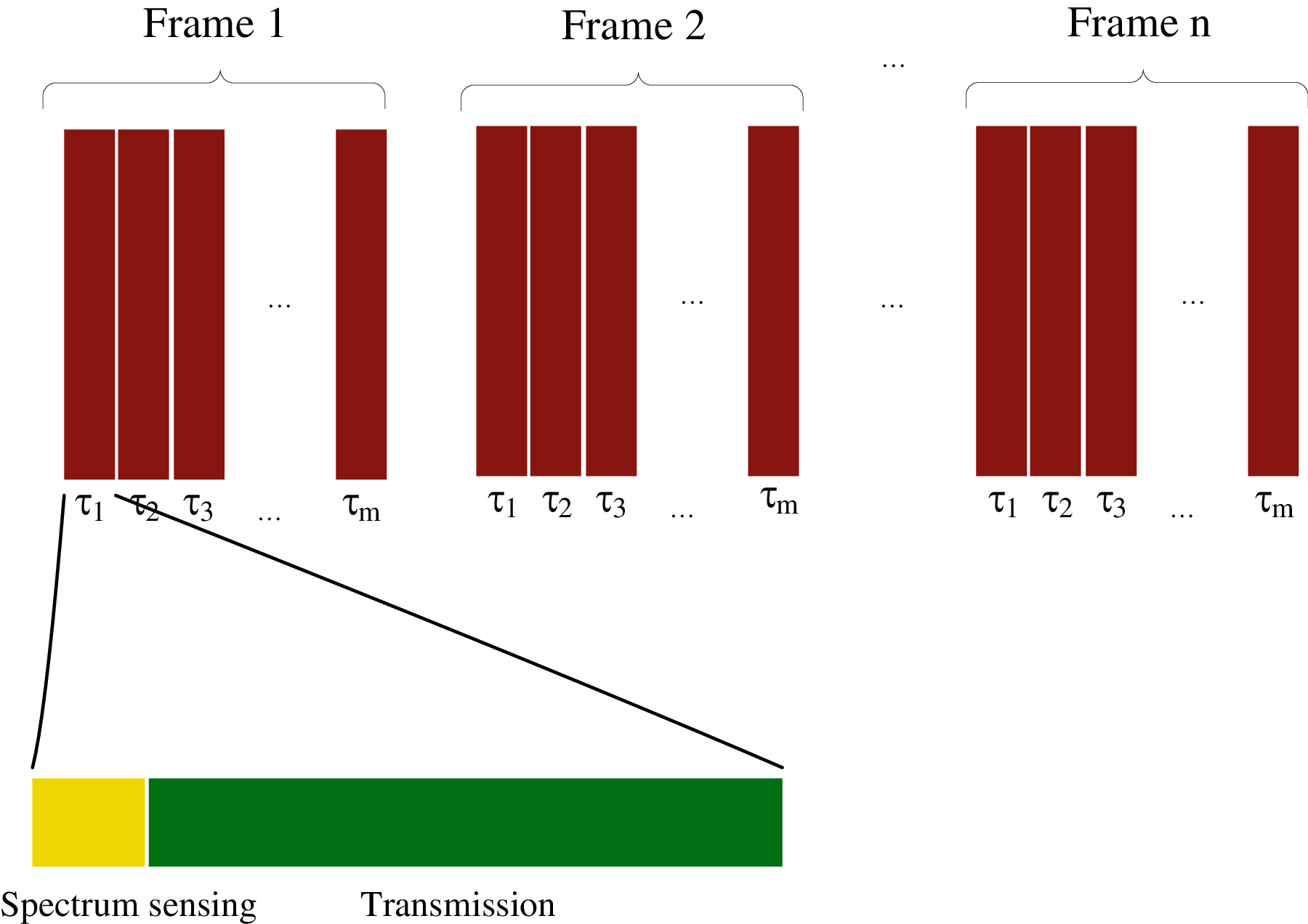
Figure 2: The structure of a frame

According to the above definition, a Cognitive Radio Sensor Network (CRSN) should have the ability to identify hot spots and manage transmission links to avoid hot spots. Based on this, this paper proposes a path selection scheme based on semi-supervised learning, which aims to accurately predict hot spots in CRSN with a limited number of samples and establish a stable communication link.

3  Proposed Scheme

In this paper, the path selection scheme is based on a semi-supervised learning algorithm, which is divided into two steps. The first step is tri-training based prediction [23], which uses historical transmission data and current spectrum sensing data to model communication reliability until the prediction accuracy reaches the threshold. The second step is a path selection algorithm which is based on the predicted results. The neighbor node with the highest reliability will be selected as the next-hop to obtain a stable communication path. Through these two steps, it can finally manage SU nodes avoid the hot spot of the PU's activities, reduce transmission interruptions and energy consumption.

3.1 Initialization

In each time slot, the SUs first perform spectrum sensing and create an Available Channel List (ACL). Meanwhile, in order to predict the link connectivity of the sink node, each SU needs to maintain one Context Information (CI) includes:

(1)   The neighbor node ID(di) and the Sind node ID(si);

(2)   Current time slot (τ1,…,τm);

(3)   Current available channel set (Ch1,Ch2,…,Chc);

Meanwhile, in order to ensure energy efficiency, the context information is collected in a passive manner. In the initialization of the network, the sink node uses the CCC to periodically broadcast HELLO messages. The HELLO message is a control data packet to establish a route path, which contains the sink node ID, the set of locally available channels, and the current time slot t.

When the SU receives the HELLO message, it compares the ACL with the sender's available channel set. If there is no common available channel, the node discards the HELLO message and no longer forward; if there is a common available channel, the node uses the information contained in the HELLO message to update the context information. That is, the ID of the sink node, the ID of the sender, and the common available to the sender channels are stored. Meanwhile, the available channel set in the HELLO message is updated with ACL and forwarded to downstream neighbors until there are no downstream neighbors. The overall flowchart of the above process is shown in Fig. 3.

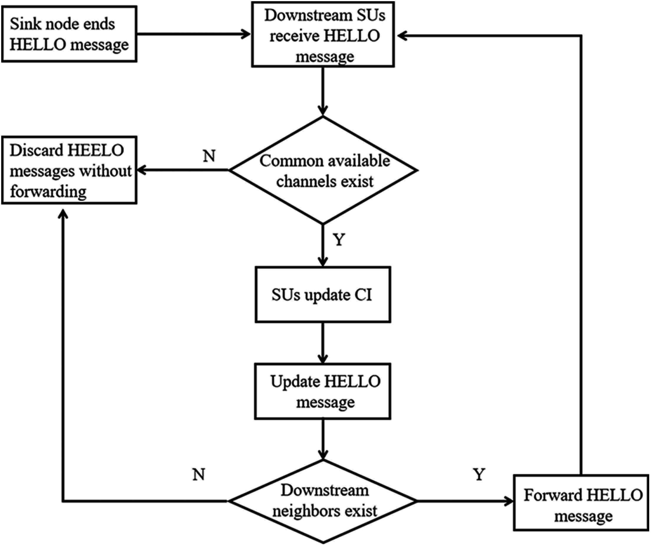
Figure 3: HELLO message forwarding process

3.2 Tri-Training Based Predicition Algorithm

3.2.1 Parameters

In summary, let U={(x1,x2,…,xM)} represent the unlabeled sample set with length M, where xk=(Si,τk,dj,Chl)T,0<k≤M indicates the neighbor node dj is selected to use the channel Chl for transmission at the time slot τk, and the ACL is traversed. Meanwhile, D={(x1,y1),(x2,y2),…,(xN,yN)} is defined to represent a labeled sample set with length N, where yk={ 0,1}  represents the result of communication with the sink node (successful/unsuccessful).

3.2.2 Transmission Availability Prediction

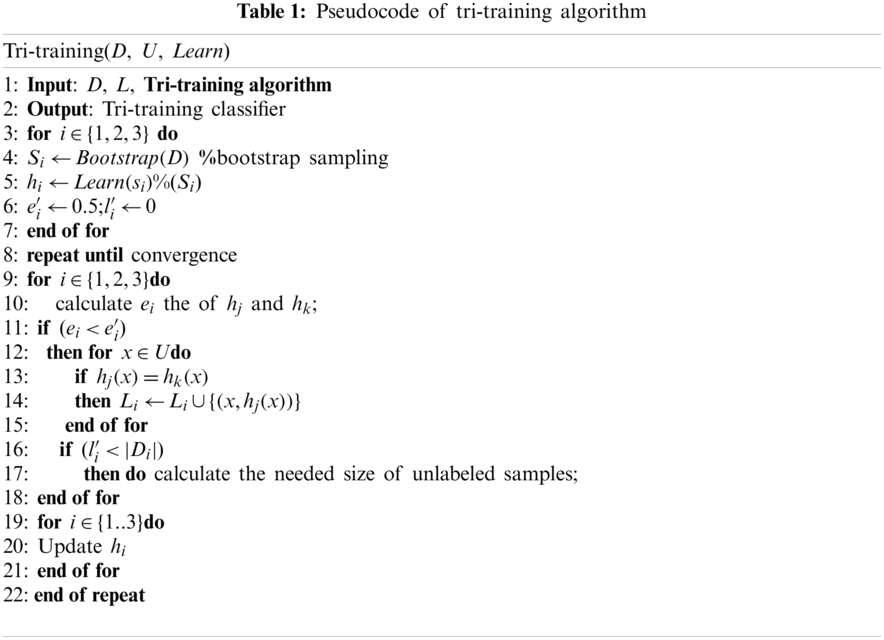
The Tri-training based prediction algorithm needs to build three classifiers and make the final result decision upon the prediction results of the three classifiers. It is divided into three steps: Bootstrap sampling, classifier training and transmission availability prediction, which are described as follows.

(1)   Bootstrap Sampling

In order to improve the diversity of classifiers, bootstrap sampling is used. Specifically, three sample groups with the same number of samples S1, S2, and S3 are randomly selected from the labeled sample set to complete the initialization of the classifier and realize the diversity of the three classifiers.

(2)   Classifier Training

After using the bootstrap sampling method to obtain the initial training set S1, S2 and S3, three classifiers h1, h2 and h3 are generated respectively. At time slot t, the unlabeled sample set is. For any classifier, as long as the other two classifiers agree with the labeled result of a certain unlabeled sample, the sample can be added to the training set for further training of the classifier. Specifically, if the sample x in the U, the pair of classifiers h2 and h3 has the same labeling results, then x can be added to the label sample set D, thereby expanding the number of training samples of the classifier h1. The definition Dk in this paper represents the sample set marked for h1 for training in the k-th round of tri-training, and the length is |Dk|.

In this case, if the prediction results of h2 and h3 are correct, the classifier h1 will obtain a valid new sample to enhance the training effect. However, when the prediction results of both are wrong, then the sample obtained by h1 is with noise. In order to solve this problem, the classification error rate of h2 and h3 needs to be calculated in the initial stage of each round of tri-training, that is:

e1k=Sum2,3−Sum2,3∗|D|,0≤Sum2,3∗≤Sum2,3≤|D|(1)

where e1t indicates the classification error rate of h2 and h3 in the k-th round, Sum2,3 indicates the number of times that the h2 and h3 have the same sample labeling, Sum2,3∗ indicates the number of times that the sample labeling results in h2 and h3 are both correct, and |D| indicates the total number of samples in the D. It should be noted that since it is difficult to confirm the truth of labeling, the calculation of the classification error rate is only performed in D. Based on formula (1), the number of incorrectly labeled samples in Dk can be calculated, and the total noise rate in k-th round can be calculated as:

ηk=ηD|D|+e1k|Dk||D∪Dk|(2)

where ηD represents the noise rate of the labeled sample set. However, since the labeled samples in this paper are true values which have been tested in transmission, thus ηD=0.

According to the theoretical derivation of literature [23], if the training effect of h1 can be improved by dk, the following conditions should be met:

|D∪Dk|(1−2e1k|Dk||D∪Dk|)2>|D∪Dk−1|(1−2e1k−1|Dk−1||D∪Dk−1|)2(3)

The condition for formula (3) is |Dk−1|<|Dk| and e1k|Dk|<e1k−1|Dk−1|, that is:

0<e1ke1k−1<|Dk−1||Dk|<1(4)

However, when e1k<e1k−1 and |Dk−1|<|Dk|, if the value of |Dk| is much greater than |Dk−1|, then the value will be not less than e1k−1|Dk−1|. When this situation happens, part of samples should be removed from Dk. The size S after removing some samples should meet:

S=⌈e1k−1|Dk−1|e1k−1⌉s.t.|Dk−1|>e1ke1k−1−e1k(5)

When the performance of the classifier h1 no longer improves, it means that the classification performance of h1 is optimal at time t. Then the above process is repeated by the classifiers h2 and h3 respectively, so that the classification performance of the three classifiers is optimal at time t.

The pseudocode of Tri-training algorithm is shown in Tab. 1.

(3)   Classification

After completing the training at time t, tri-training algorithm uses voting method for each common available channel with each neighbor node to make a transmission availability decision. The channel can be successfully transmitted is classified as “1”, otherwise it is “0”, and for all public channels. Then the total number of successful transmission number between neighbor nodes and sink nodes selected by the SU at time t can be calculated as Tratdk.

Different from the traditional tri-training algorithm, this paper has modified its mechanism partially, that is, after the tri-training classifier classifies the communication reliability at time t, the node will randomly select an available neighbor node and common idle channel for transmission, and add the transmission result (successful or unsuccessful) to D. In other words, the labeled sample set is continuously expanding until the classification accuracy of tri-training reaches the predetermined threshold.

3.2.3 Communication Reliability Based Path Selection Scheme

After the SU calculates the total number of successful transmissions from neighbor nodes dk and sink nodes at time t, total number of successful transmissions of all neighbor nodes can be calculated. The total number of successful transmission between the SU and the sink node at time t as the SU is defined as the communication reliability:

relti=∑kTratdk(6)

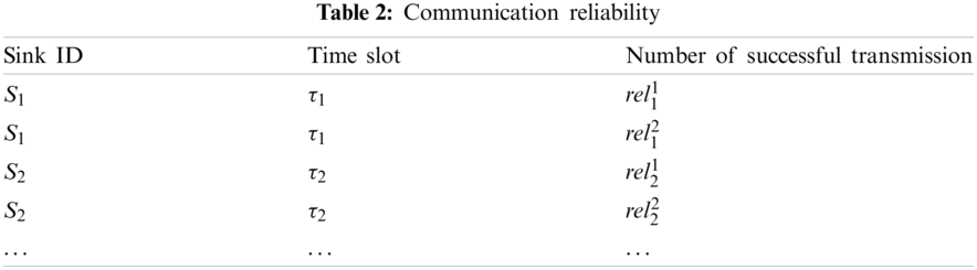
The SU calculates the communication reliability between the neighbor node and the sink node in each time slot in the frame and generates the communication reliability table shown in Tab. 2.

When a SU needs to communicate with a sink node, it will broadcast a Routing Request (RREQ) message, which contains the sink node ID and the currently available channels. After the neighbor node receives the message, if there is an available channel, it adds its own ID and communication reliability to the message, adds the reliable channel in the message to its own ACL, and broadcasts the message to the neighbor node; otherwise, it discards the message. The sink node finally receives the RREQ message forwarded by multiple paths, and establishes the topology structure according to the message, preferentially selects the node with the highest communication reliability to establish the transmission path, and sends a Route Reply (RREP) message containing the path node ID along the path.

As shown in Fig. 4, each node has a communication reliability value. For example, when the PU moves at time T2, it affects the SUs d7. At this time, the communication reliability of the node d7 is 2, and the node with higher reliability is first selected as the relay node for transmission, that is d5, then the path is (d4→d5→d6→d8→sink). The overall process is shown in Fig. 5.

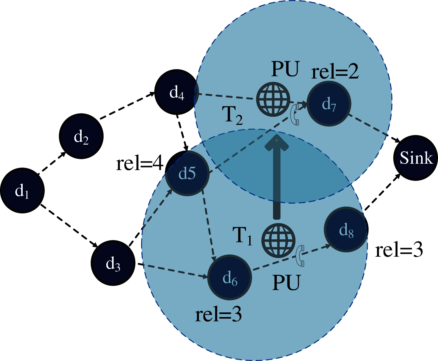
Figure 4: Path reliability of the network

4  Simulation Results

In this section, the performance of the proposed tri-training based scheme is evaluated in terms of energy consumption and spectrum utilization through simulations. The simulation environment consists of 10 SUs and one Sink deployed within a 50 m*50 m area, and the communication range of each SU is set to 20 m. It is assumed that each SU can transmit to the Sink directly or through several intermediate SU nodes, and each frame consists of 60 time slots. Moreover, both the total energy consumption by an SU and the throughput in one transmission are normalized to one for visual comparison.

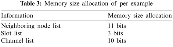
Three classifiers, i.e., Decision Tree (DT), Logistic Regression (LR) and Gradient Boosting Decision Tree (GBDT) are employed to form the tri-training algorithm. A Pure Gradient Routing (PGR) scheme without tri-training based scheme is used for comparison. In the PGR scheme, all SUs will perform spectrum sensing every time slot and determine starting transmission or not. Moreover, each example generated for training contains 3 bytes of information, as depicted in Tab. 3.

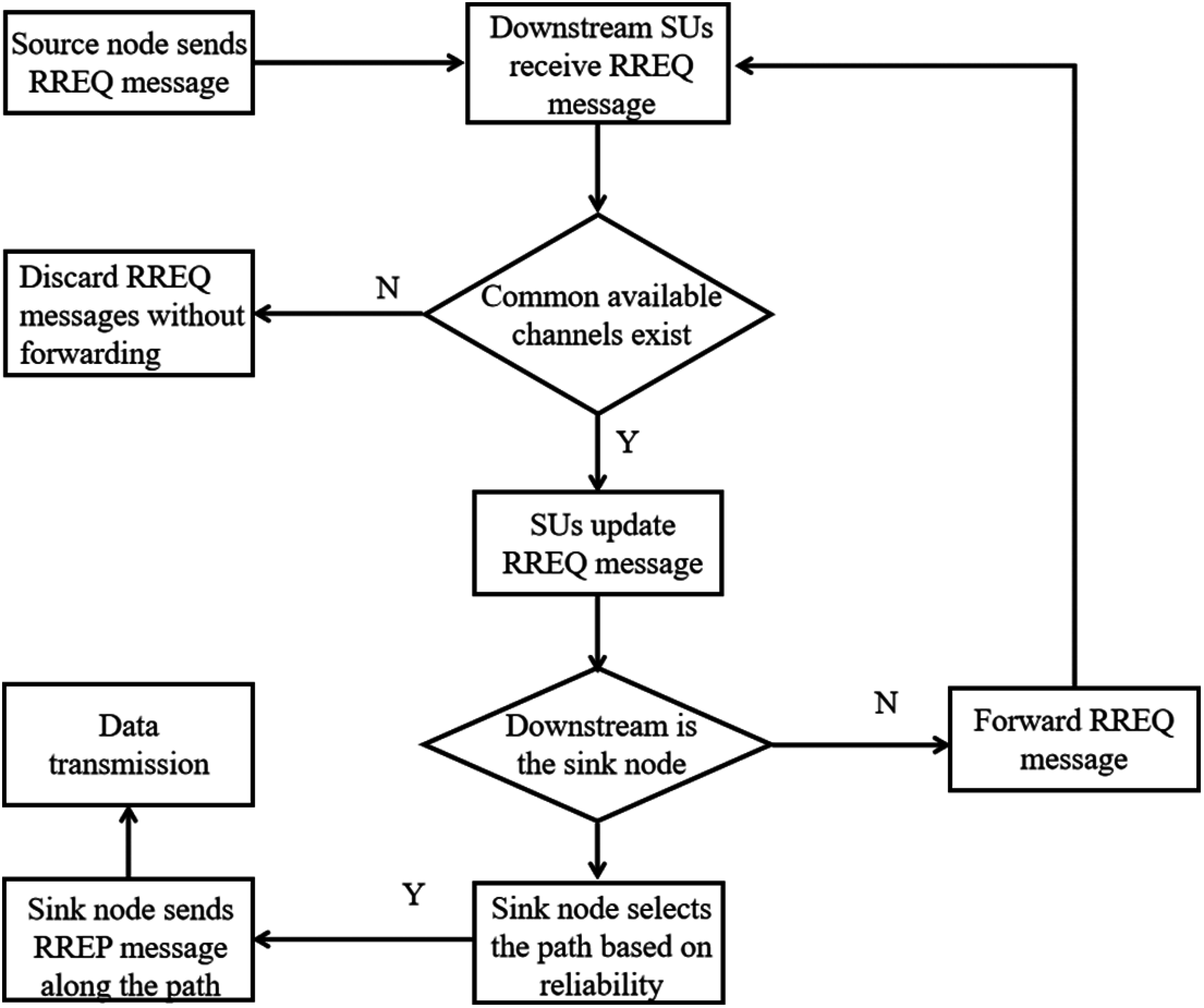
Figure 5: The process of path building

The simulation runs for over 600 rounds (frames), each round consists of 60 time slots.

Fig. 6 compares the prediction precision of the proposed scheme against the three classifiers that make it up. As can be seen, the prediction precision of both tri-training and the three classifiers increases while the number of labeled examples in training phases increases. Meanwhile, the precision of tri-training is higher than any of the three classifiers (DT, LR and GBDT) under the same labeled examples.

Since the memory size of cognitive radio devices is limited, it is necessary to control the total size of labeled examples. Thus, the precision of tri-training under different memory size of labeled examples is shown in Fig. 7. While the precision threshold is set to 96%, the tri-training algorithm requires about 45 KB memory size to store the label examples and that is acceptable for a cognitive radio device.

Fig. 8 compares the communication reliability of the two path selection schemes. In order to prevent the arrival rate of the PUs from being too low and causing too little impact on CRSN. The initial value of λ is 0.15, while avoiding excessive disparity in the intensity of the PUs’ activities, the value of λ in each round of simulation is 0.15 to 0.5.

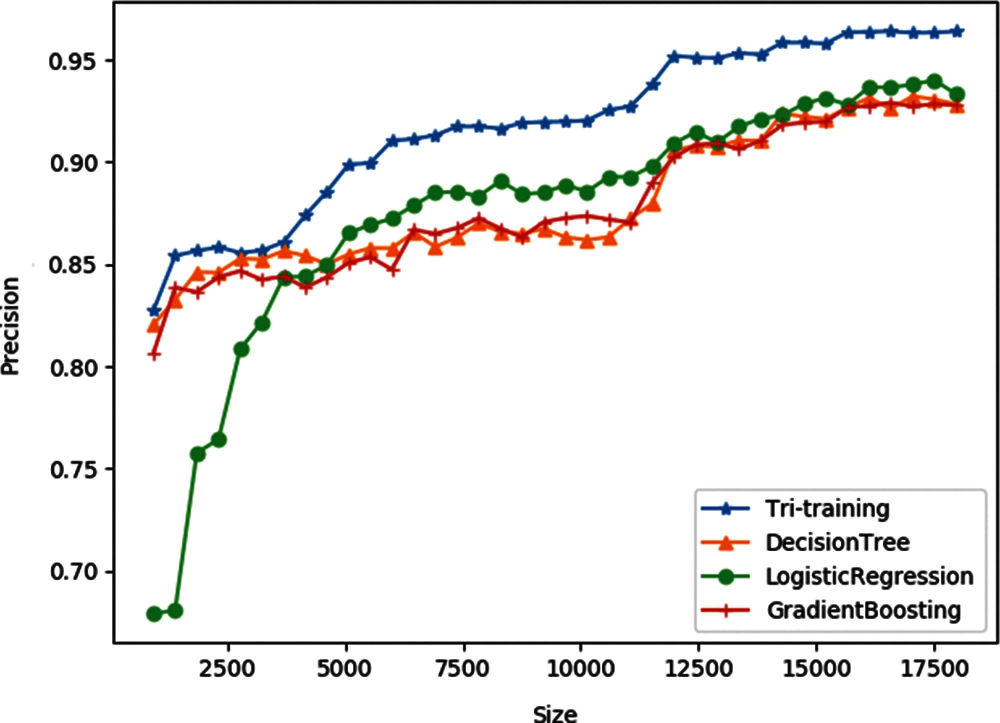
Figure 6: Comparison of classification precision of different classifiers

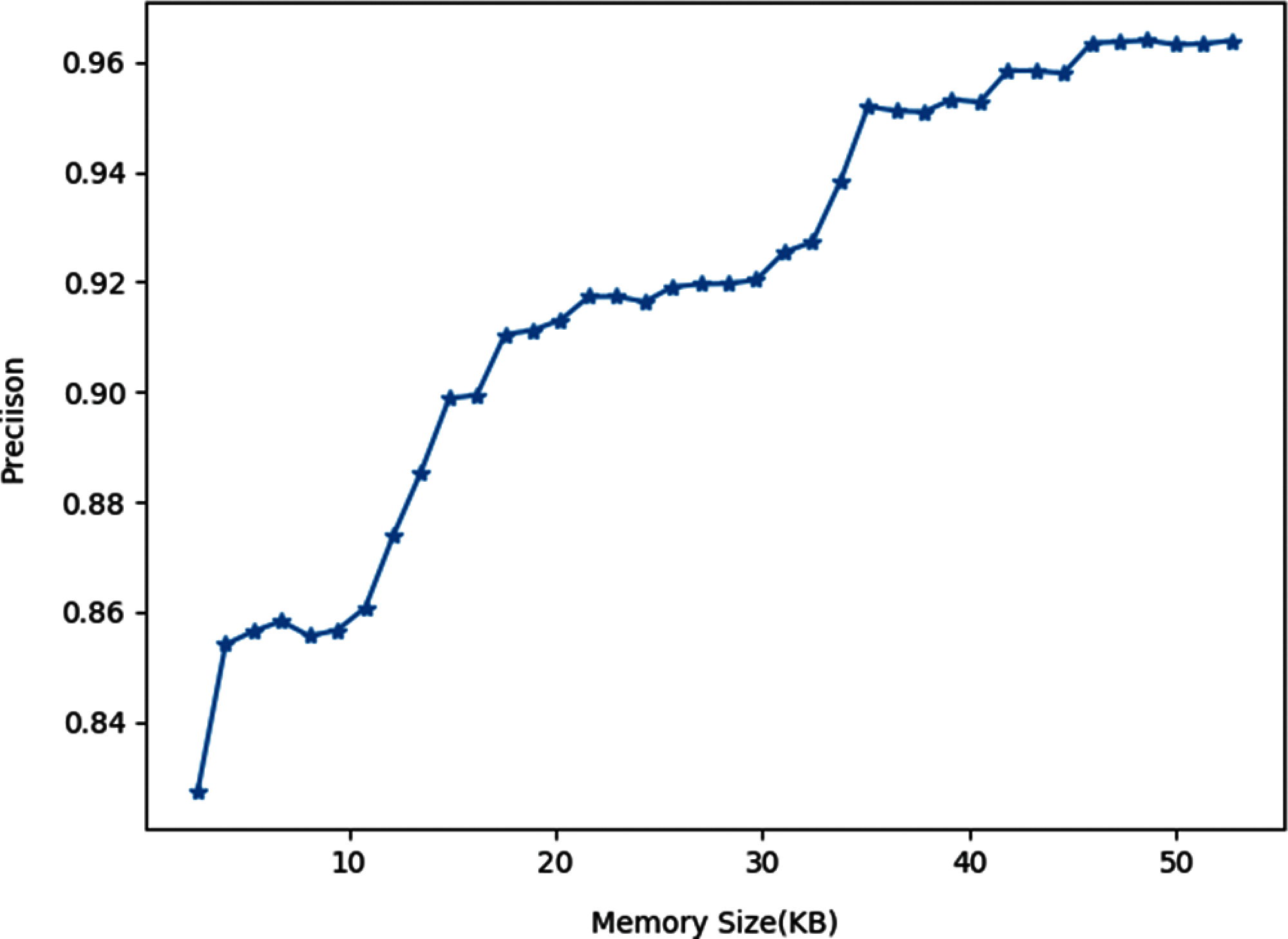
Figure 7: Precision of tri-training under different memory size of labeled examples

It can be seen from the figure that when the network selects the shortest path algorithm spectrum aware mesh routing (SAMER), the data packet transfer ratio is unstable. This is because SAMER selects the path with many common channels and the shortest path based on the spectrum sensing result, and the spectrum sensing result is not perfect. At the same time, the shortest path is affected by PU's activities. The greater the frequency of main user activities, the greater the path interruption frequency and the lower the data packet transmission rate. As the simulation is performed, the average packet transmission rate of SAMER converges to 55%. In contrast, the proposed tri-training-based path selection algorithm shows a more stable packet transmission rate, and the average performance converges to 84%. Compared with SAMER, the performance of the scheme proposed in this paper is 29% higher.

The result is mainly due to two reasons. First, the proposed prediction algorithm based on tri-training can intelligently estimate the communication reliability of the link. Secondly, the path selected by the path selection algorithm based on transmission reliability has the least possibility of interruption. In addition, the proposed method can effectively avoid the influence of PUs, and therefore can also effectively avoid additional energy consumption due to frequent retransmissions.

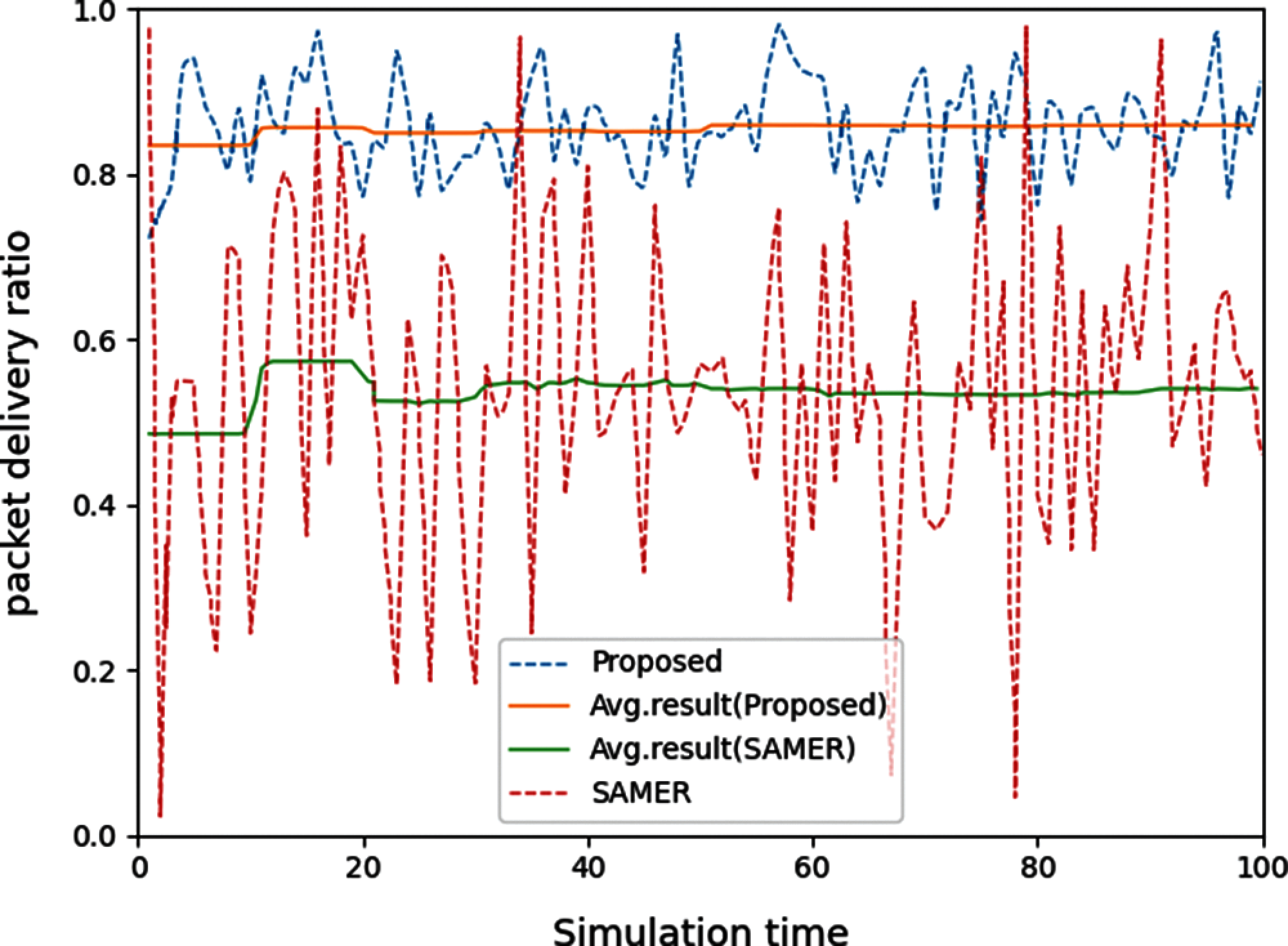
Figure 8: Data packet transfer ratio

Fig. 9 compares energy consumption of the proposed scheme and the PGR scheme. As can be seen, energy consumption of the tri-training based scheme is lower than the PGR scheme. This is because the PGR scheme performs spectrum sensing and data exchange in each time slot resulting in higher energy consumption, while the proposed scheme can utilize the duty-cycle mechanism to save energy. In this simulation, the parameter λ is set to 0.3, which means if the ratio of available time slots in a frame is predicted to be more than 30%, then SU in this frame will keep active. Thus, the SUs will stop spectrum sensing and data exchanging if γ is less than 0.3 which resulting in less consumption.

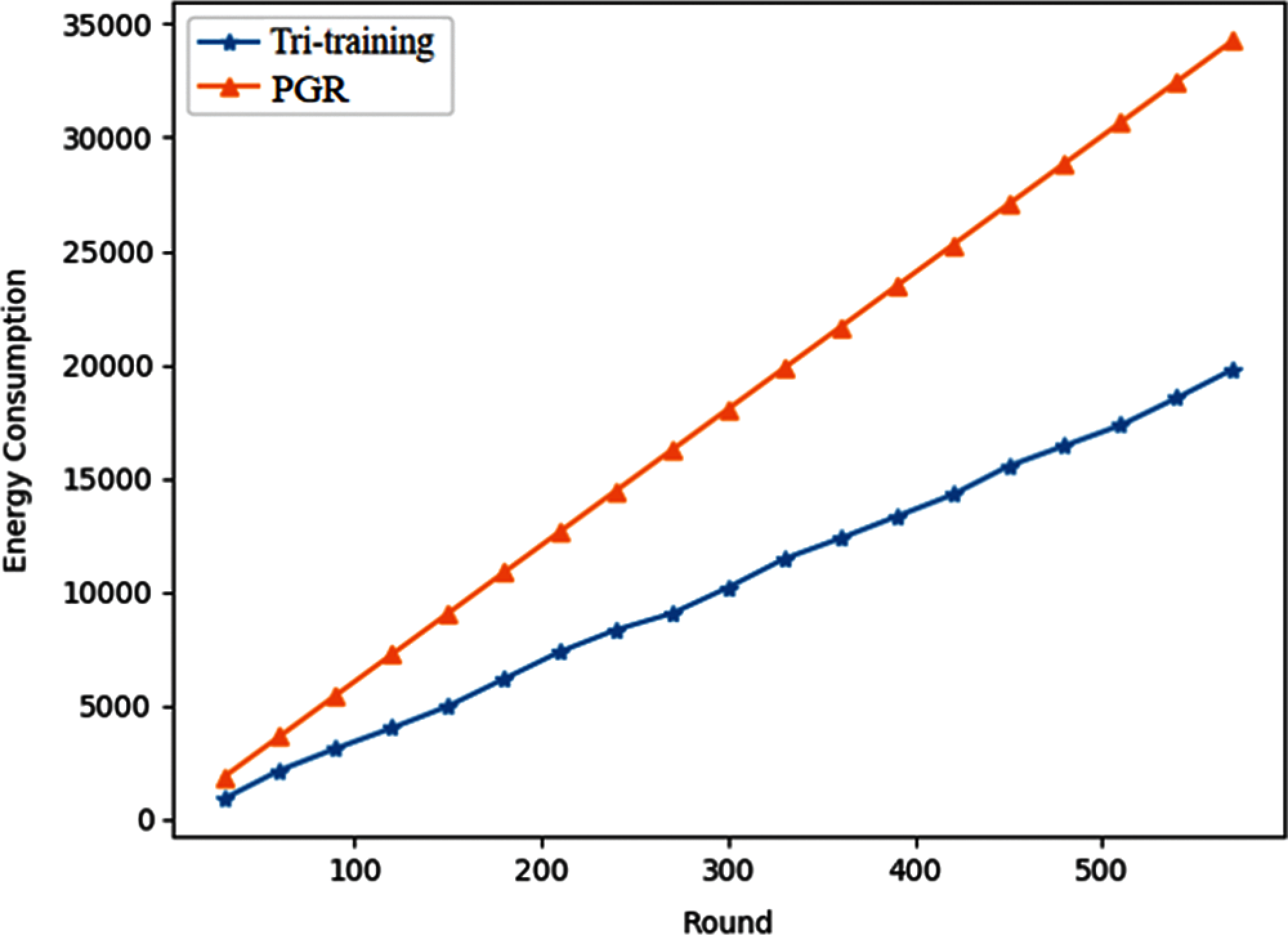
Figure 9: Energy consumption of the proposed scheme and the PGR scheme

Fig. 10 shows that the PGR scheme outperforms the proposed scheme in terms of throughput and this is caused by the duty-cycle mechanism. Due to duty-cycle mechanism, the proposed scheme will stop operating in some busy frames which results in missing transmission chances. However, the PGR scheme keeps operating in these frames and the available time slots for transmission can be utilized.

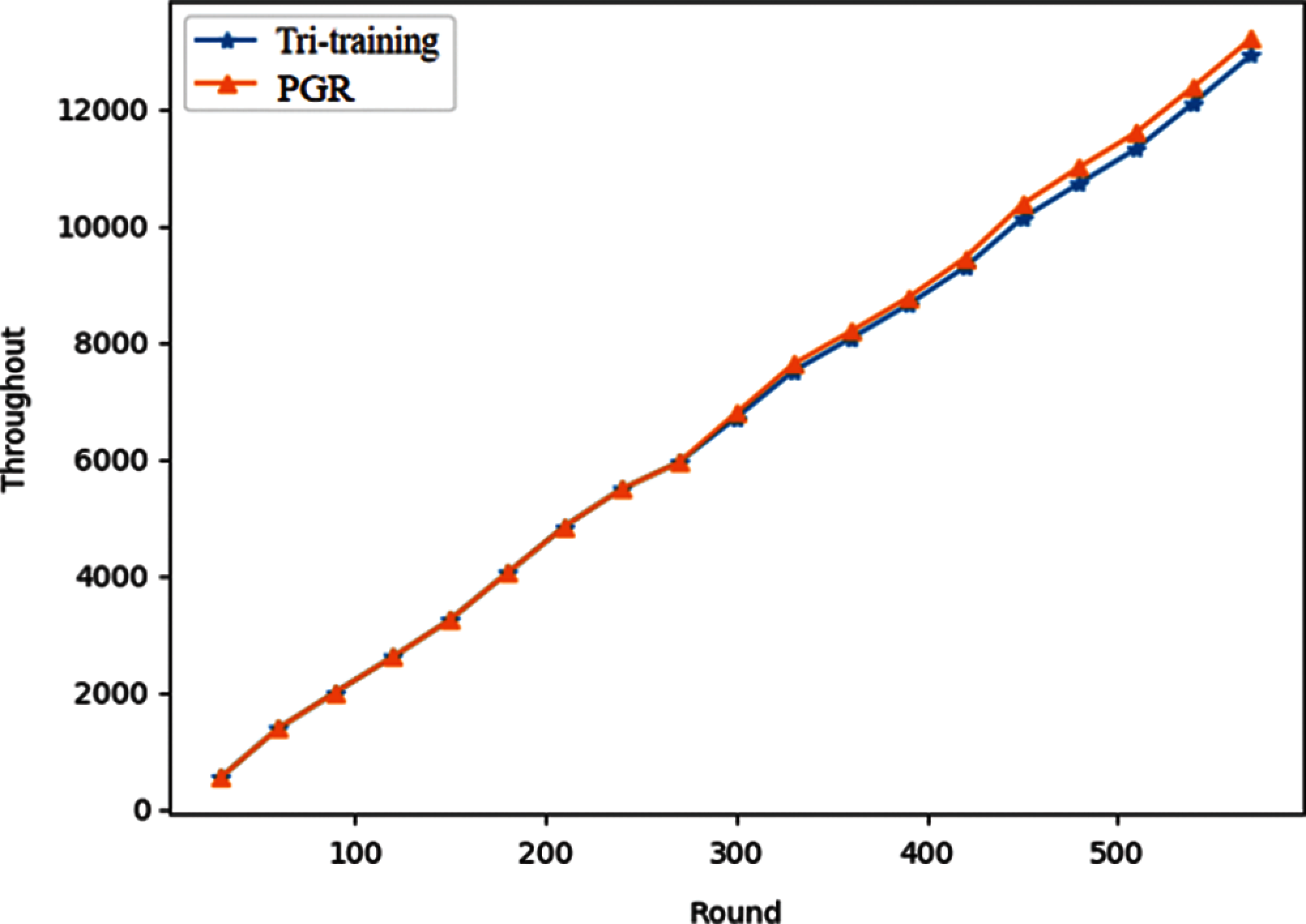
Figure 10: Throughput of the tri-training and PGR scheme

Although the tri-training based scheme can reduce the energy consumption, the network throughput is also reduced. This relationship can be defined using the throughput-energy rate, which is given as:

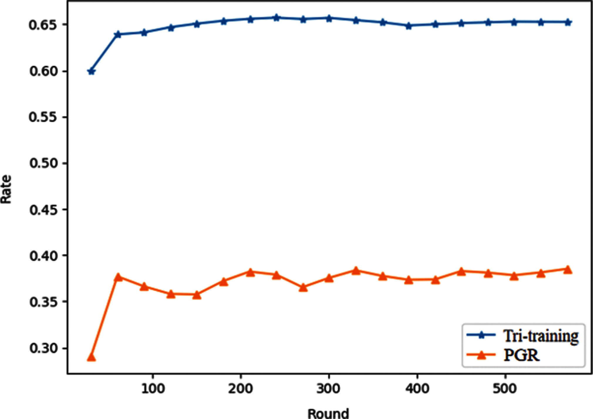
Figure 11: Throughput-energy rates

∑i=0nThroughputi∑i=0nETi(7)

where n is the number of rounds, and Throughouti is the throughput in i−th round.

In other words, high throughput and low energy consumption result in a high throughput-energy rate which means better network performance.

Fig. 11 shows that the proposed algorithm has a higher throughput-energy rate compared with the PGR scheme. Therefore, the proposed tri-training based scheme has better network performance.

5  Conclusion

This paper introduced a tri-training based algorithm which focuses on an intermediate node selection approach for cognitive radio networks. The number of labeled examples for training can be reduced through the tri-training algorithm, and the energy consumption can be reduced by the optimized duty-cycle mechanism. The simulations were performed to verify the performance of the proposed scheme. However, our experiments are still not sufficient. As a future work, the stable routing issue will be addressed combined with the proposed tri-training scheme.

Funding Statement: This work was partially supported by the National Natural Science Foundation of China (Grant Nos. 11761074, 61972207, 61902041), the Natural Science Foundation of Jilin Province of China (Grant No. 2020122336JC), Project of Jilin Science and Technology Development for Leading Talent of Science and Technology Innovation in Middle and Young and Team Project (No. 20200301053RQ) and the Project through the Priority Academic Program Development (PAPD) of Jiangsu Higher Education Institution.

Conflicts of Internet: The authors declare that they have no conflicts of interest to report regarding the present study.

References

 1.  J. Mitola and G. Q. Maguire, “Cognitive radio: Making software radios more personal,” IEEE Pers Commun, vol. 6, no. 4, pp. 13–18, 1999.

 2.  S. Haykin, “Cognitive radio: Brain-empowered wireless communications,” IEEE Journal on Selected Areas in Communications, vol. 23, no. 2, pp. 201–220, 2005.

 3.  H. Huang, Z. Y. Zhang, P. Cheng and P. L. Qiu, “Opportunistic spectrum access in cognitive radio system employing cooperative spectrum sensing,” in Proc. of IEEE Vehicular Technology, Barcelona, Spain, 2009.

 4.  Y. Zhang, J. Liu, Y. Peng, Y. Dong, G. Sun et al., “Performance analysis of relay based noma cooperative transmission under cognitive radio network,” Computers, Materials & Continua, vol. 63, no. 1, pp. 197–212, 2020.

 5.  H. Q. Wang, E. H. Yang, Z. J. Zhao and W. Zhang, “Spectrum sensing in cognitive radio using goodness of fit testing,” IEEE Transactions on Wireless Communications, vol. 8, no. 11, pp. 5427–5430, 2009.

 6.  F. L. Tang, M. Y. Guo, S. Guo and C. Z. Xu, “Mobility prediction based joint stable routing and channel assignment for mobile ad hoc cognitive networks,” IEEE Transactions on Parallel and Distributed Systems, vol. 27, no. 3, pp. 789–802, 2016.

 7.  M. Cesana, F. Cuomo and E. Ekici, “Routing in cognitive radio networks: Challenges and solutions,” Ad Hoc Networks, vol. 9, no. 3, pp. 228–248, 2011.

 8.  S. Tabatabaei, “A novel fault tolerance energy-aware clustering method via social spider optimization (sso) and fuzzy logic and mobile sink in wireless sensor networks (wsns),” Computer Systems Science and Engineering, vol. 35, no.6, pp. 477–494, 2020.

 9.  Y. Yang, Q. Zhao, L. Ruan, Z. Gao, Y. Huo et al., “Oversampling methods combined clustering and data cleaning for imbalanced network data,” Intelligent Automation & Soft Computing, vol. 26, no.5, pp. 1139–1155, 2020.

10. C. B. Liu, K. L. Li and K. Q. Li, “A game approach to multi-servers load balancing with load-dependent server availability consideration,” IEEE Transactions on Cloud Computing, vol. 9, no. 1, pp. 1–13, 2021.

11. R. Doost-Mohammady, M. Y. Naderi and K. R. Chowdhury, “Spectrum allocation and QoS provisioning framework for cognitive radio with heterogeneous service classes,” IEEE Transactions on Wireless Communications, vol. 13, no. 7, pp. 3938–3950, 2014.

12. X. L. He, H. Jiang, Y. Song, C. L. He and H. Xiao, “Routing selection with reinforcement learning for energy harvesting multi-hop CRN,” IEEE Access, vol. 7, pp. 54435–54448, 2019.

13. Y. B.Qu, C. Dong, H. P. Dai, F. Wu, S. J. Tang et al., “Network coding-based multicast in multi-hop CRNs under uncertain spectrum availability,” in Proc. of IEEE Conf. on Computer Communications (INFOCOMHong Kong, China, pp. 783–791, 2015.

14. K. L. Li, X. Y. Tang and K. Q. Li, “Energy-efficient stochastic task scheduling on heterogeneous computing systems,” IEEE Transactions on Parallel and Distributed Systems, vol. 25, no. 11, pp. 2867–2876, 2014.

15. E. Chatziantoniou, B. Allen and V. Velisavljević, “An HMM-based spectrum occupancy predictor for energy efficient cognitive radio,” in Proc. of IEEE 24th Annual Int. Symposium on Personal, Indoor, and Mobile Radio Communications, London, UK, 2013.

16. H. Eltom, S. Kandeepan, Y. C. Liang, B. Moran and R. J. Evans, “HMM based cooperative spectrum occupancy prediction using hard fusion,” in Proc. of IEEE Int. Conf. on Communications Workshops (ICCKuala Lumpur, Malaysia, 2016.

17. A. Saad, B. Staehle and R. Knorr, “Spectrum prediction using hidden markov models for industrial cognitive radio,” in Proc. of Wireless and Mobile Computing, Networking and Communications (WiMobNew York, NY, USA, 2016.

18. M. Monemian, M. Mahdavi and M. J. Omidi, “Optimum sensor selection based on energy constraints in cooperative spectrum sensing for cognitive radio sensor networks,” IEEE Sensors Journal, vol. 16, no. 6, pp. 1829–1841, 2016.

19. O. Ergul and O. B. Akan, “Cooperative coarse spectrum sensing for cognitive radio sensor networks,” in Proc. of IEEE Wireless Communications and Networking Conf. (WCNCIstanbul, Turkey, 2014.

20. J. Ren, Y. X. Zhang, Q. Ye, K. Yang, K. Zhang et al., “Exploiting secure and energy-efficient collaborative spectrum sensing for cognitive radio sensor networks,” IEEE Transactions on Wireless Communications, vol. 15, no. 10, pp. 6813–6827, 2016.

21. S. Parvin and T. Fujii, “A novel spectrum aware routing scheme for multi-hop cognitive radio mesh networks,” in Proc. of IEEE 22nd Int. Symposium on Personal, Indoor and Mobile Radio Communications, Toronto, ON, Canada, 2011.

22. A. Jamal, C. Tham and W. Wong, “CR-Wsn MAC: an energy efficient and spectrum aware MAC protocol for cognitive radio sensor network,” in Proc. of 9th Int. Conf. on Cognitive Radio Oriented Wireless Networks and Communications (CROWNCOMOulu, Finland, 2014.

23. Z. H. Zhou and M. Li, “Tri-training: Exploiting unlabeled data using three classifiers,” IEEE Transactions on Knowledge and Data Engineering, vol. 17, no. 11, pp. 1529–1541, 2005.

This work is licensed under a Creative Commons Attribution 4.0 International License, which permits unrestricted use, distribution, and reproduction in any medium, provided the original work is properly cited.