Computers, Materials & Continua DOI:10.32604/cmc.2022.021382
Article

SutteARIMA: A Novel Method for Forecasting the Infant Mortality Rate in Indonesia

Ansari Saleh Ahmar1,2,*, Eva Boj del Val3, M. A. El Safty4, Samirah AlZahrani4 and Hamed El-Khawaga5,6

1Business School, Faculty of Economics and Business, Universitat de Barcelona, Barcelona, 08034, Spain
2Department of Statistics, Faculty of Mathematics and Natural Science, Universitas Negeri Makassar, Makassar, 90224, Indonesia
3Department of Economic, Financial and Actuarial Mathematics, Faculty of Economics and Business, Universitat de Barcelona, Barcelona, 08034, Spain
4Department of Mathematics and Statistics, Colleage of Sciences, Taif University, P.O. Box 11099, Taif, 21944, Saudi Arabia
5Department of Statistics, Mathematics, and Insurance, Faculty of Commerce, Tanta University, Egypt
6Department of Economics and Finance, College of Business Administration, Taif University, P.O. Box 11099, Taif, 21944, Saudi Arabia
*Corresponding Author: Ansari Saleh Ahmar. Email: ansarisaleh@unm.ac.id
Received: 12 June 2021; Accepted: 17 August 2021

Abstract: This study focuses on the novel forecasting method (SutteARIMA) and its application in predicting Infant Mortality Rate data in Indonesia. It undertakes a comparison of the most popular and widely used four forecasting methods: ARIMA, Neural Networks Time Series (NNAR), Holt-Winters, and SutteARIMA. The data used were obtained from the website of the World Bank. The data consisted of the annual infant mortality rate (per 1000 live births) from 1991 to 2019. To determine a suitable and best method for predicting Infant Mortality rate, the forecasting results of these four methods were compared based on the mean absolute percentage error (MAPE) and mean squared error (MSE). The results of the study showed that the accuracy level of SutteARIMA method (MAPE: 0.83% and MSE: 0.046) in predicting Infant Mortality rate in Indonesia was smaller than the other three forecasting methods, specifically the ARIMA (0.2.2) with a MAPE of 1.21% and a MSE of 0.146; the NNAR with a MAPE of 7.95% and a MSE of 3.90; and the Holt-Winters with a MAPE of 1.03% and a MSE: of 0.083.

Keywords: Forecasting; infant mortality rate; ARIMA; NNAR; holt-winters; SutteARIMA

1  Introduction

In this era of globalization and continuous industrial development, every human being wants to get information as fast as possible. Statistics, which is one of the fields of science related to the acquisition of information in several scientific disciplines, has made progress. This advancement usually requires different methods of solving different problems. Statistics has been known for a long time and has even been used in dealing with problems in everyday life such as in the fields of health, economics, social sciences, atmospheric sciences, and other fields. In addition, the development of data mining and big data analysis also requires an understanding of statistics. This is in line with the opinion of Sivarajah, Kamal, Irani, and Weerakkody [1] in their presentation depicted in Fig. 1. Fig. 1 shows that the types of classification of big data analytical methods, especially in the descriptive analytical, inquisitive and predictive analytical sections require statistical analysis to obtain information. Furthermore, Grover & Mehra [2] stated that data mining is the application of statistics in the form of exploratory analysis and modeling of data to obtain shapes and trends from large data sets.

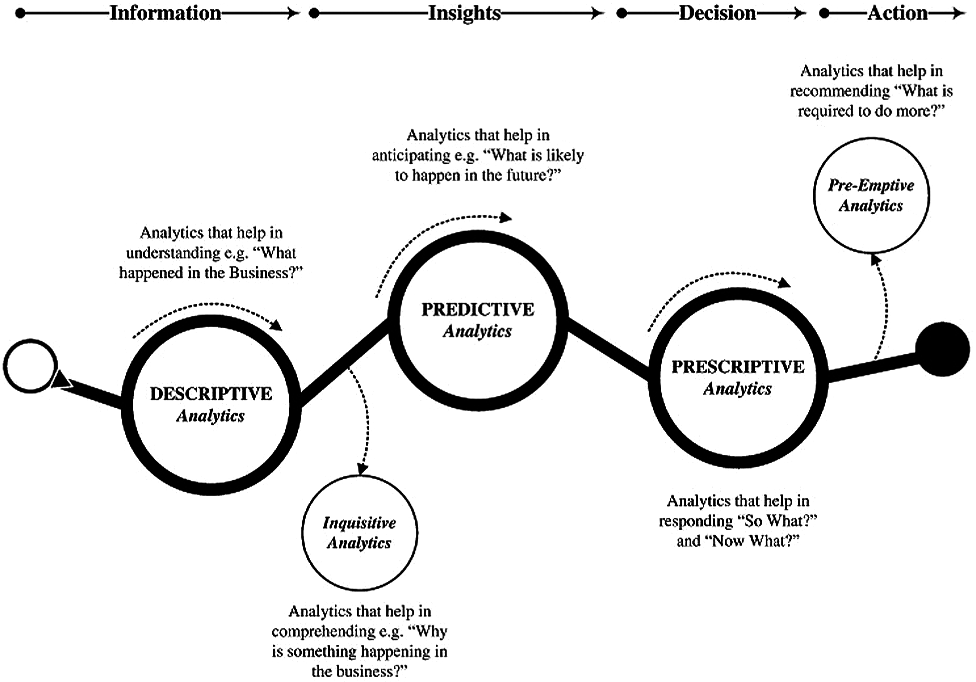
Figure 1: Classification of big data analytical method types [1]

Statistics are usually used by data analysts to consider possible events that may recur. Therefore, the likelihood of future events is strongly influenced by the frequency and routine of events that have occurred in the past. This is in line with the opinion of Edwards [3] who states that predictive analysis is data analysis that aims to make predictions about future events based on historical data and analysis techniques. Based on this, it can be said that statistics has a connection with events in the past that may recur in the future. The statistical method that is often used to obtain future information is known as forecasting or predictive analysis. Predictive analysis is often employed in economics, finance, health, and other fields [4,5].

In the health sector, forecasting is often used as a means of evaluating the implementation, success and failure of a health program or health service that is being implemented. In addition, forecasting is also often used as a means of planning and decision making in the implementation of future activities. For example, Ranapurwala [6] used predictive modeling in the field of public health, namely agricultural vehicle accidents and concluded that forecasting or predictive data will be able to assist health policy makers (government, doctors, and health practitioners) in making decisions in an effort to improve public health; El Safty [7] and El Safty et al. [8] used modeling in corona virus topic using topological method. On the other hand, forecasting methods can also be applied to several topics in the health sector, such as birth and death rates. The incidence of birth and death in an area is commonly used as an indicator in assessing the success of health services and health development programs in an area.

The infant mortality rate is one of the health problems in Indonesia that needs to be highlighted, because the infant birth rate is one of the indicators commonly used in determining public health. It is not surprising that health programs in Indonesia focus a lot on the problem of infant mortality, namely the reduction in infant mortality rates. In 2008, the Infant Mortality Rate in Indonesia was still quite high, around 31/1000, or in other words, 31 babies died in every 1,000 births. This mortality rate is higher when compared to Malaysia and Singapore, which amounted to 16.39/1000 and 2.3/1000 live births, respectively.

According to WHO data, in 2019, globally, as many as 7000 newborns died every day and 185 cases per day occurred in Indonesia with an infant mortality rate of 24 per 1000 live births, with details of 75% of neonatal deaths occurring in the first week, and 40% died within the first 24 h [9]. Given the importance of this infant mortality rate and to achieve one of the targets of the sustainable developmental goals (SDGs) in the health sector of the Republic of Indonesia, namely by 2030, to end preventable deaths of newborns and children under five, with all countries trying to reduce the Neonatal Mortality Rate at least up to 12 per 1000 KH (Live Birth) and the under-five mortality rate of 25 per 1000, a suitable statistical method is needed in order to provide information in the future to minimize infant mortality. One of the statistical methods that is suitable for this problem of infant mortality is the method of prediction. Due to a decreasing trend from year to year, the infant mortality rate in Indonesia is assumed to meet the trend pattern. Forecasting methods that are suitable for the trend method are the ARIMA [10], Neural Networks [11], Holt-Winters [11], and SutteARIMA [12]. SutteARIMA is used in this study because the SutteARIMA method is a new forecasting method that has a good level of accuracy in some forecasting data [12].

2  Literature

2.1 ARIMA Method

The Autoregressive Integrate Moving Average (ARIMA) model was first discovered and presented by George Box and Gwilym Jenkins in 1976, and their names are often synonymous and associated with the ARIMA process applied for time series analysis, namely ARIMA Box-Jenkins. In general, the ARIMA model is written with the ARIMA notation (p, d, q), where p represents the order of the autoregressive process (AR), d represents the differencing, and q represents the order of the moving average (MA) process.

2.1.1 AR Process

The autoregressive model is a form of regression that connects the observed values at a certain time with the values of previous observations at certain intervals [13].

In general, the autoregressive process of data at the p level (AR (p)) [14]:

Zt=ϕ1Zt−1+ϕ2Zt−2+…+ϕpZt−p+at,at∼WN(0,σ2),ϕi∈R,t∈ZZt=ϕ1BZt+ϕ2B2Zt+…+ϕpBpZt+at,at∼WN(0,σ2),ϕi∈R,t∈Z(1−ϕ1B+ϕ2B2+…+ϕpBp)Zt=at,at∼WN(0,σ2),ϕi∈R,t∈Z(1)

This equation can be simplified into ϕP(B)Zt=at, where ϕP(B)=1−ϕ1B+ϕ2B2+…+ϕpBp.

Because of this ∑j=1∞|πj|=∑j=1p|ϕj|<∞ then this process is always invertible, for stationary, then the root of ϕP(B)=0 must be outside the unit circle.

2.1.2 MA Process

The moving average process is a process that functions to describe phenomena in which the event produces an immediate effect which only lasts for a short period of time. The model of the general process moving average (MA) is as follows [13]:

Zt=at−θ1at−1−θ2at−2−…−θqat−1,at∼WN(0,σ2),θi∈R,t∈ZZt=at−θ1Bat−θ2B2at−…−θqBqat,at∼WN(0,σ2),θi∈R,t∈ZZt=(1−θ1B−θ2B2−…−θqBq)at,at∼WN(0,σ2),θi∈R,t∈Z(2)

or

Zt=θQ(B)at,at∼WN(0,σ2),θi∈R,t∈Z(3)

With:

θQ(B)=1−θ1B−θ2B2−…−θqBq(4)

Because 1−θ1B−θ2B2−…−θqBq<∞ then the finite moving average process is always stationary. This moving average process will be declared invertible if the root from θQ(B)=0 is outside of the circle.

2.1.3 ARMA Process

The model of the moving average autoregressive process (ARMA) [13]:

Zt=ϕ1Zt−1+ϕ2Zt−2+…+ϕpZt−p+at−θ1at−1−θ2at−2−…−θqat−1,at∼WN(0,σ2),ϕi∈R,t∈ZZt=ϕ1BZt+ϕ2B2Zt+…+ϕpBpZt+at−θ1Bat−θ2B2at−…−θqBqat,at∼WN(0,σ2),ϕi∈R,t∈Z(1−ϕ1B+ϕ2B2+…+ϕpBp)Zt=(1−θ1B−θ2B2−…−θqBq)at,at∼WN(0,σ2),ϕi∈R,t∈ZϕP(B)Zt=θQ(B)at,at∼WN(0,σ2),ϕi∈R,t∈Z(5)

With:

ϕP(B)=1−ϕ1B+ϕ2B2+…+ϕpBp(6)

and

θQ(B)=1−θ1B−θ2B2−…−θqBq(7)

For an invertible process, it is required that the root of θQ(B)=0 outside of the unit circle. And in order for it to be stationary, it is necessary that the root of ϕP(B)=0 it outside of the unit circle. It is also assumed ϕP(B)=0 and θQ(B)=0 don't have the same root. Furthermore, this process is referred to as the ARMA (p, q) model or process, where p and q are used to denote the respective order of polynomial values associated with autoregressive and moving averages.

2.1.4 ARIMA Process

The ARIMA process is basically similar to the ARMA process, they state that stationary and invertible processes can be represented in the form of a moving average or in an autoregressive form in the ARMA section. AR, MA, and ARMA require that data must be stationary, both in mean and in variance. Data can be stated as stationary in terms of average, if the time series data is relatively constant over time, it is stated to be stationary in variance, if the time series data structure from time to time has constant or constant data fluctuations and does not change or does not change the variance in the magnitude of the fluctuation. To overcome this non-stationary mean, a differencing process is carried out, and for non-stationary variants, a power transformation is carried out. (λ). In the ARIMA modeling process, the variance stationarity process is carried out first then the average stationarity. From this stationary process comes the ARIMA process.

This ARIMA contains a differencing process to stationary data that is not stationary in the mean in the ARMA process. If there is a d-order differencing, then to achieve a stationary and general model of the ARIMA process (0, d, 0) it becomes:

(1−B)dZt=at,at∼WN(0,σ2),d,t∈Z(8)

and from this equation, we can form a general model of the ARIMA process (p, d, q):

ϕP(B)(1−B)dZt=θQ(B)at,at∼WN(0,σ2),θi,ϕi∈R,d,t∈Z(9)

With the AR stationary operator ϕP(B)=1−ϕ1B−ϕ2B2−ϕpBpand invertible MA operator θQ(B)=1−θ1B−θ2B2−…−θqBq with no common factors.

2.1.5 The Stages in Forecasting the ARIMA(p, d, q)

In the execution of time Series data forecasting, the ARIMA method (p, d, q) have steps or stages. The stages in forecasting are as follows [14].

Model identification

Model identification is done to see the meaning of autocorrelation and data stationarity, to determine whether or not it is necessary to carry out a transformation or a differencing process (differentiation). From this stage, a temporary model will be obtained from which the process of testing the model will be carried out whether it is appropriate or not on the data.

Model Assessment and Testing

After the model identification process has been carried out, the next step is to assess and test the model. This stage consists of two parts, namely parameter assessment and model diagnostic examination.

a)   Parameter Assessment

After obtaining one or more provisional models, the next step is to find estimates for the parameters in that model.

b)   Model Diagnostic

Diagnostic checking is done to check whether the estimated model is quite suitable or adequate with the existing data. Diagnostic checking is based on residual analysis. The basic assumption of the ARIMA model is that the residual is an independent random variable with a normal distribution with a constant mean of zero variance.

(1)   Independent Test

This independent test is performed using the Box-Pierce Q statistical test. The Box-Pierce Q test can be calculated using the formula [14]:

Q=n∑k=1mρk2(10)

where: n = amount of data

ρk = autocorrelation for lag k, k = 1, 2, …, m

If the value is Q<χm−p−q2, it is considered that the model is adequate, and vice versa, if the value is Q>χm−p−q2, it is considered inadequate.

(2)   Normality Test

Residual analysis is used to examine whether the residuals of the model are white noise or not. White noise is the basic assumption of the ARIMA model where the residual in this case is a free random variable that is normally distributed with zero mean and constant variance.

2.2 Holt-Winters Method

Holt-Winters is a method for modeling and predicting the behavior of data from a time series. In addition, Holt-Winters is one of the most used time series forecasting methods. It is decades old, but is still widely used in a variety of applications, including monitoring, which is used for things like anomaly detection and capacity planning. The Holt-Winters model uses three aspects of the time series: a typical value (average)/stationary, trend, and seasonality. Because it uses these three aspects, Holt-Winters is also known as triple exponential smoothing. Holt-Winters uses three smoothing parameters, namely α, β, γ, each of which has a value between 0 – 1.

The formula of Holt-Winters [15]:

Seasonal Smoothing:

SNt=γ(XtSt)+(1−γ)SNt−L(11)

Smooting Data:

St=αXtSNt−1+(1−α)(St−1+Tt−1)(12)

Trend Smooting:

Tt=β(St−St−1)+(1−β)Tt−1(13)

Forecast:

Ft+m=(St+Ttm)SNt−L+m(14)

Ft+m=(αXtSNt−1+(1−α)(St−1+Tt−1)+β(St−St−1)+(1−β)Tt−1m)γ(XtSt)Ft+m=+(1−γ)SNt−1(15)

with:

Xt = actual data at time t,

St = data smoothing value,

St − 1 = previous data smoothing value,

Tt = trend smoothing

Tt − 1 = smoothing of the previous period's trend,

SNt = seasonal smoothing,

SNt − 1 = the previous period's seasonal smoothing,

α = exponential parameter for smoothing data with a value between 0 and 1,

β = exponential parameter for trend smoothing with a value between 0 and 1,

γ = exponential parameter for seasonal smoothing with a value between 0 and 1,

Ft + m = forecast value,

m = the time period to be predicted,

L = seasonal length.

2.3 Neural Network

An artificial neural network (ANN) is a system that processes information with characteristics and performance close to that of a biological neural network. Artificial neural networks are a generalization of biological neural network modeling with several assumptions, including:

a) Information processing lies in a number of components called neurons.

b) The signal spreads from one neuron to another via a connecting line.

c) Each connecting line has a weight and multiplies the value of the incoming signal (certain types of neurons).

d) Each neuron implements an activation function (usually nonlinear) which adds up all the inputs to determine the output signal.

Neural networks are useful for estimating or regression analysis including for forecasting and modeling, classification including pattern recognition and sequence recognition, as well as for decision making in sorting and processing data including filtering, grouping, and compression as well as programming of robots that move independently without human assistance. According to Wuryandari et al. [16], an artificial neural network model is determined by:

a) Patterns of relationships between neurons (network architecture)

b) The method for determining and changing the joint weights is called the training method or network learning process

c) Activation function

Artificial neural networks are also known as brain metaphors, computational neuron science, and parallel distributed processing. Neural networks are used for complex non-linear forecasting. One of the network requirements related to the Time Series is NNAR (Neural Network Autoregressive). Time series lag values can be used as input to neural networks, such as the lag values used in linear autoregressive models. This method is known as the neural network autoregressive model (NNAR). The NNAR model is generally denoted by NNAR (p, k) where p = input lag and k = number of hidden layers and NNAR (p, P, k) is the general denotation for NNAR in seasonality. For example, the NNAR (4, 3) is a neural network that has four observational data (yt−1, yt−2, …, yt−4) which serve as input data used to predict the outcome or value of forecasting (Yt), and is accompanied by three neurons in a hidden layer.

The NNAR model is a feed-forward neural network that involves a combination of linear and activation functions. This function formulation is defined as:

netj=∑iwijyij(16)

f(y)=11+e−y(17)

2.4 SutteARIMA Method

SutteARIMA is a short-term forecasting method developed by Ahmar et al in 2019 [17]. This method is a hybrid method between α-Sutte Indicator and ARIMA.

The formula of SutteARIMA [17]:

Zt=α(ϕ12+Δz3α+3β)+β(ϕ32+2Δy3β+3γ)+γ(ϕ32+2Δx3γ+3δ)+ϕ4δ2+…+ϕpZt−p2+at2−θ1at−12−θ2at−22−…−θqat−q2(18)

3  Methodology and Data

3.1 Dataset

In this paper, we use annual time series data from Mortality rate, infant (per 1,000 live births) for Indonesia which is obtained from the World Bank Database. Data for this paper is available at: https://data.worldbank.org/indicator/SP.DYN.IMRT.IN?locations=ID. The World Bank website contains different annual time series at various levels of aggregation, from 1960–2019. In conducting data analysis, the data is divided into two parts, namely training data (from 1960–2012) and fitting/testing data (from 2013–2019). Training data is used to obtain forecasting models and fitting data is used to see the level of accuracy of the forecasting models obtained in the training data. Data were analyzed using forecasting methods: ARIMA, Neural Networks Time Series, Holt-Winters, and SutteARIMA method. To simplify the analysis, we used the R Software version 3.6.3, namely the SutteForecastR package and Microsoft Excel 2010.

3.2 Forecast Accuracy

In the results of the fitting/testing data, two performance indicators or forecasting accuracy are used to assess the quality with the good of fit standard and the accuracy of the forecasting results obtained. The indicators are as follows [18].

- Mean Absolute Percentage Error (MAPE)

MAPE=1n∑t=1n|At−FtAt|(19)

- Mean Square Error (MSE)

MSE=∑t=1n(At−Ft)2n(20)

where:

At = Actual values at data time t.

Ft = Forecast values at data time t.

4  Results and Discussion

In the case of infant mortality rates, the data obtained is in the form of a trend and has decreased every year (see Fig. 2). Fig. 2 shows that the data on infant mortality in 2003 and 2004 were constant and then in 2005 decreased slowly until 2019.

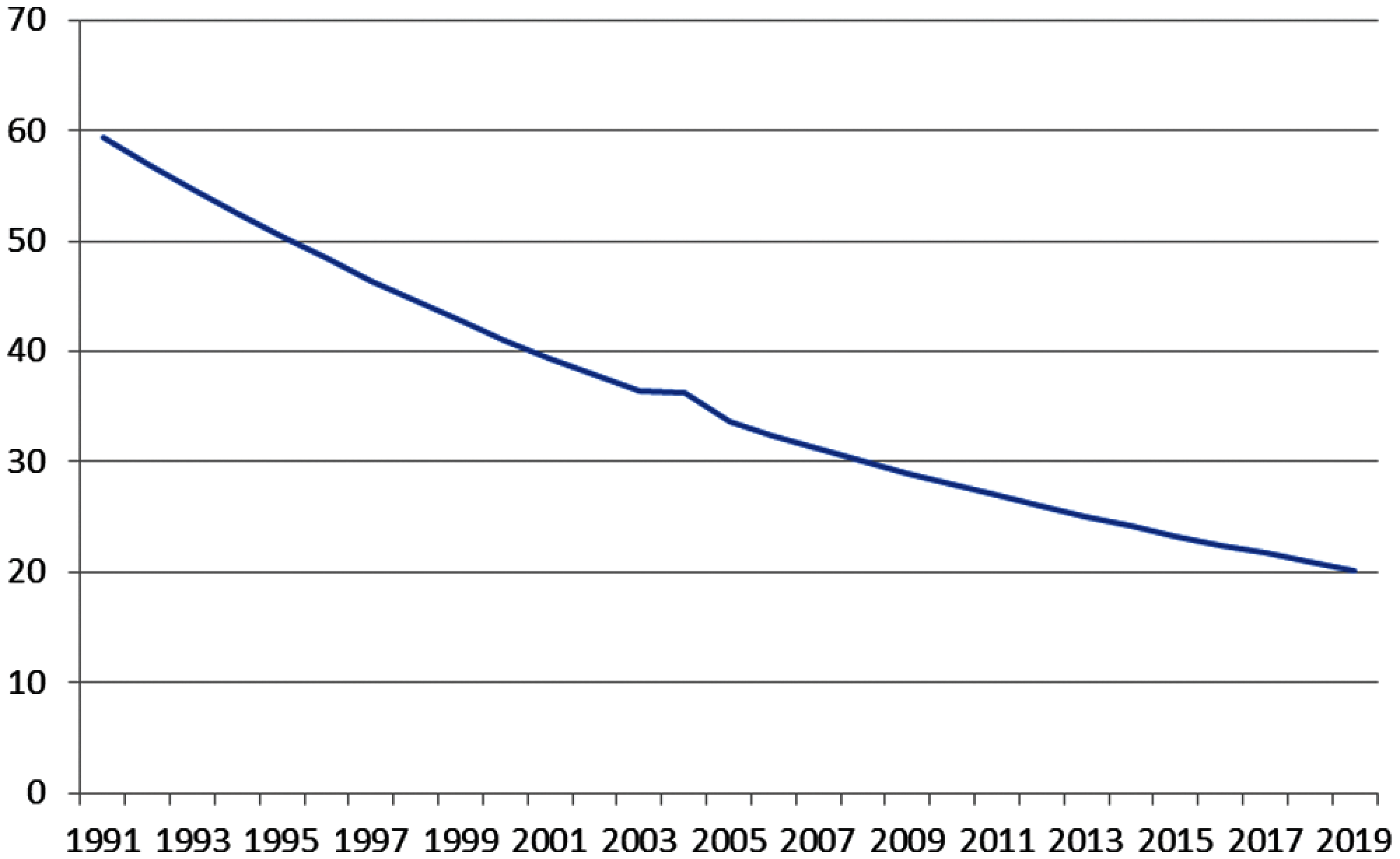
Figure 2: Infant mortality rates in indonesia

4.1 Model Specification

To obtain forecasting models and forecasting results from data using ARIMA, Neural Network Time Series, Holt-Winter, and SutteARIMA models, we use the alpha.sutte function on SutteForecastR package on Software and the output results from R Software are presented as follows.

4.1.1 Forecasting Using ARIMA Method

$Forecast_AutoARIMA

Point Forecast  Lo 80  Hi 80   Lo 95  Hi 95

23   25.05055 24.44849 25.65261 24.12978 25.97132

24   24.11898 23.31295 24.92502 22.88626 25.35171

25   23.18742 22.07214 24.30271 21.48174 24.89310

26   22.25586 20.75409 23.75763 19.95910 24.55262

27   21.32430 19.37637 23.27223 18.34520 24.30340

28   20.39274 17.94907 22.83641 16.65547 24.13001

29   19.46118 16.47840 22.44395 14.89941 24.02294

$AutoARIMA

Series: al_mi_10

ARIMA(0,2,2)

Coefficients:

    ma1 ma2

   −1.1098 0.5000

s.e.   0.2471 0.2149

sigma2 estimated as 0.2207: log likelihood=-12.88

AIC = 31.76  AICc = 33.26  BIC = 34.75

From the results of the analysis output, it is obtained the ARIMA model (0, 2, 2) with 2 times differencing and the values of MA (1): −1.1098 and MA (2): 0.5000. The form of the model is as follows.

4.1.2 Forecasting Using Neural Network Time Series Method

$Forecast_NNETAR

Point   Forecast

23    25.40859

24    24.90951

25    24.49229

26    24.14630

27    23.86136

28    23.62803

29    23.43788

$NNETAR

Series: al_mi_10

Model: NNAR(1,1)

Call:   nnetar(y = al_mi_10)

Average of 20 networks, each of which is

a 1–1–1 network with 4 weights

options were - linear output units

sigma2 estimated as 0.1567

Similar to the ARIMA method, the Neural Network Time Series method is obtained by a forecasting model, namely NNAR (1, 1) with 1 hidden screen.

4.1.3 Forecasting Using Holt-Winters Method

$Forecast_HoltWinters

Point   Forecast  Lo 80    Hi 80    Lo 95    Hi 95

23   25.0594324.5314025.5874524.2518825.86698

24   24.1523723.4704224.8343323.1094125.19533

25   23.2453222.3157924.1748521.8237224.66691

26   22.3382621.0909623.5855620.4306824.24584

27   21.4312019.8124623.0499418.9555523.90685

28   20.5241518.4900022.5583017.4131923.63511

29   19.6170917.1294922.1046915.8126423.42154

$HoltWinters

Holt-Winters exponential smoothing with trend and without seasonal component.

Call:

HoltWinters(x = al_mi_10, gamma = FALSE)

Smoothing parameters:

 alpha: 0.4384154

 beta: 0.8642498

 gamma: FALSE

Coefficients:

     [,1]

a 25.9664829

b −0.9070558

From the analysis for forecasting using the Holt-Winters method (Tab. 3), the Holt-Winters method for this data on infant mortality is Holt-Winters without seasonal components or using only two parameters, namely α = 0.4384154 and β = 0.8642498.

4.1.4 Forecasting Using SutteARIMA Method

$Tes_Data

[1] 25.1 24.2 23.3 22.5 21.7 20.9 20.2

$Forecast_AlphaSutte

[1] 25.01820 24.15097 23.28372 22.41644 21.64915 20.88184 20.11449

$Forecast_AutoARIMA

Point   Forecast  Lo 80     Hi 80     Lo 95   Hi 95

23     25.05055 24.44849 25.65261 24.12978 25.97132

24     24.11898 23.31295 24.92502 22.88626 25.35171

25     23.18742 22.07214 24.30271 21.48174 24.89310

26     22.25586 20.75409 23.75763 19.95910 24.55262

27     21.32430 19.37637 23.27223 18.34520 24.30340

28     20.39274 17.94907 22.83641 16.65547 24.13001

29     19.46118 16.47840 22.44395 14.89941 24.02294

$Forecast_SutteARIMA

Point Forecast Low 95 High 95

23   25.0344  23.7827  26.2861

24   24.1350  22.9282  25.3417

25   23.2356  22.0738  24.3973

26   22.3362  21.2193  23.4530

27   21.4867  20.4124  22.5611

28   20.6373  19.6054  21.6692

29   19.7878  18.7984  20.7772

4.2 Estimating the Forecasting Model

After obtaining the forecasting model in the specification model section, the result of forecasting for testing data are shown in Tabs. 1--4. The forecasting results are compared with the testing data to obtain the value of absolute percentage error (APE) and square of error (SE).

4.3 Model's Forecasting Performance Comparison

Based on the results of forecasting for testing data from various prediction methods that have been presented previously, the comparison of the forecasting results is presented in Fig. 3. In Fig. 3 it can be seen that SutteARIMA has the highest level of accuracy in predicting infant mortality rates. This was followed by the Holt-Winters, ARIMA(0, 2, 2), and NNAR(1, 1). The results of the forecasting graphs of each forecasting method for testing data are presented in Fig. 4. From Fig. 4, it can be seen that the ARIMA(0, 2, 2), Holt-Winters, and SutteARIMA methods go hand in hand as shown in Fig. 4 which shows MSE and MAPE results. In fact, these three methods are close to or not too far away and differ from the NNAR(1, 1) whose forecasting is inaccurate with the testing data. Based on these results, SutteARIMA is used as a method for forecasting the next 5 periods or years (Tab. 5).

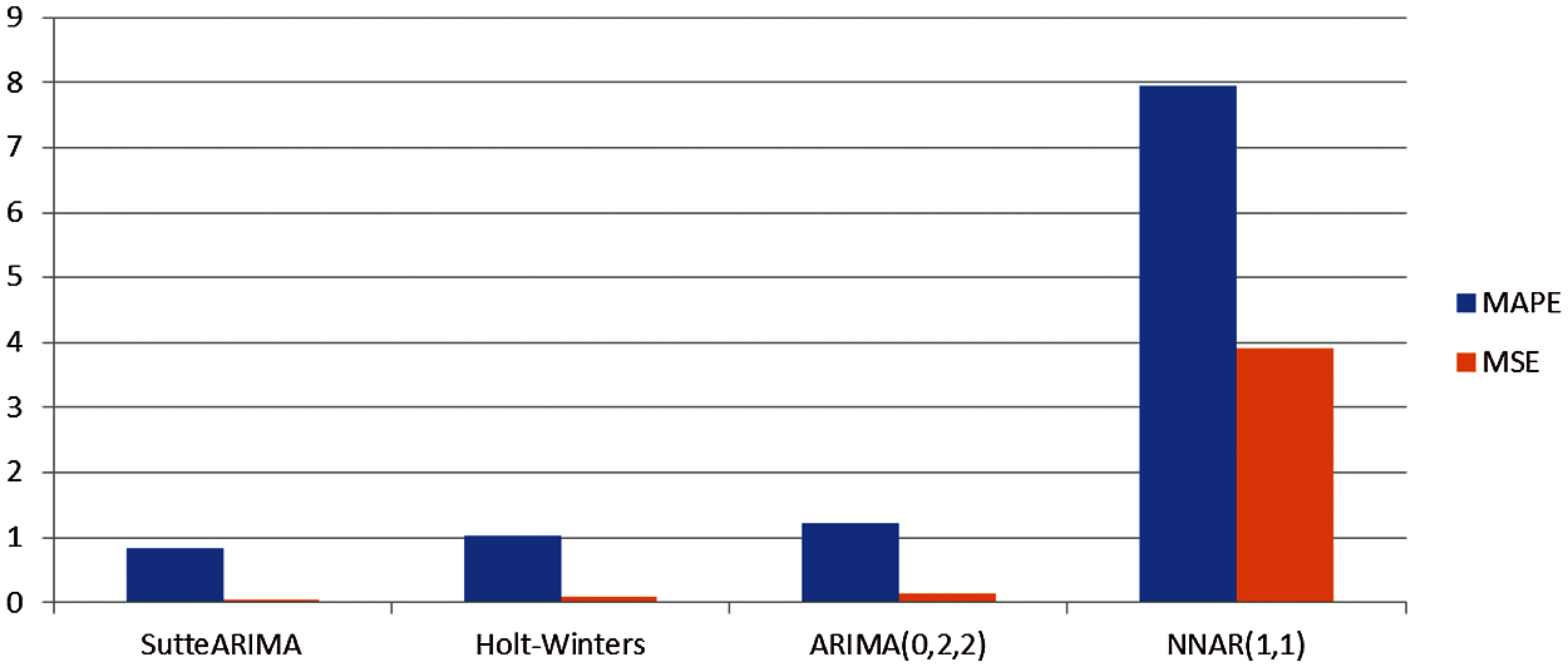
Figure 3: Comparison of forecasting accuracy on infant mortality rate in indonesia

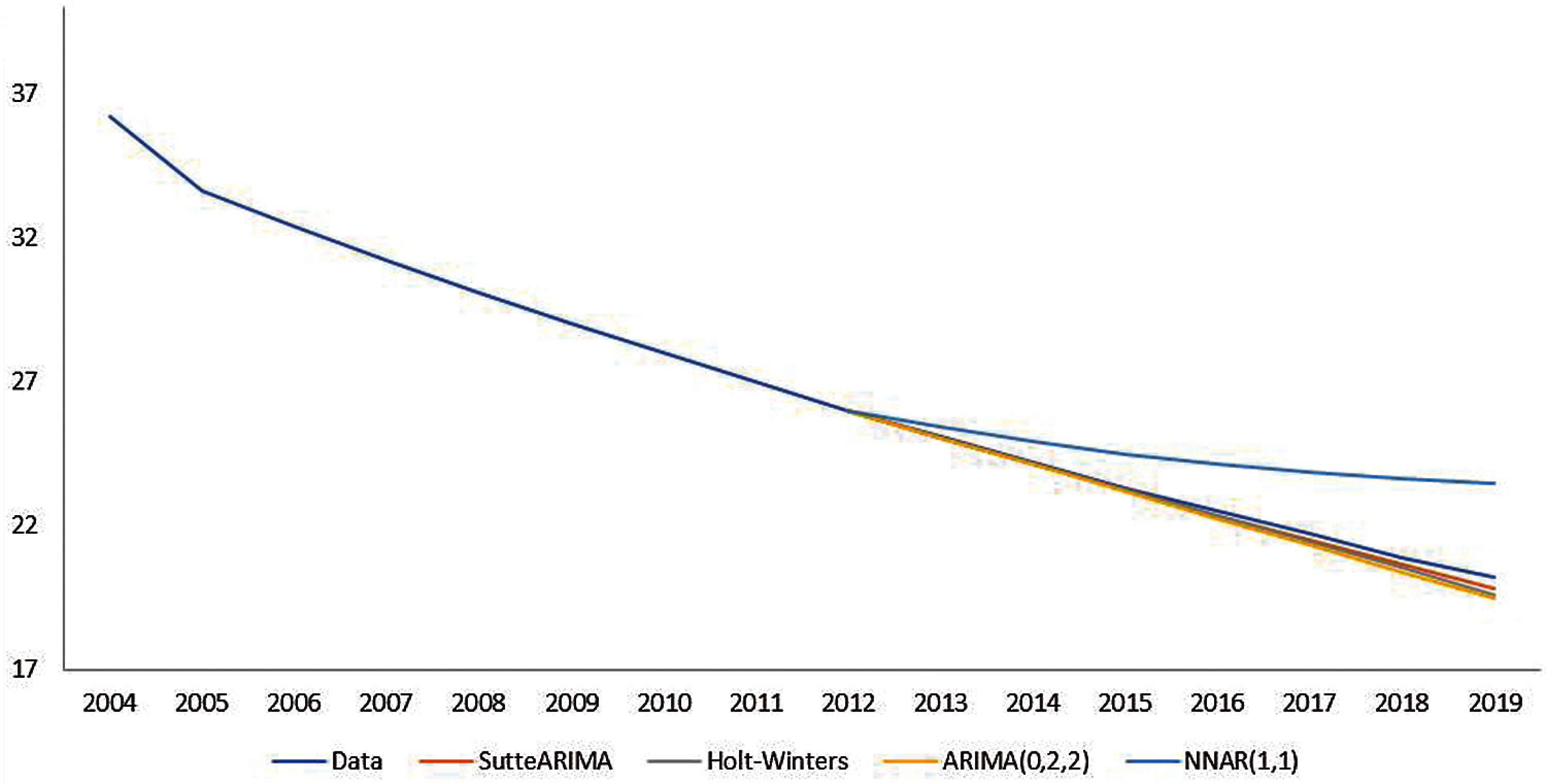
Figure 4: Testing data forecasting results on infant mortality rates in indonesia

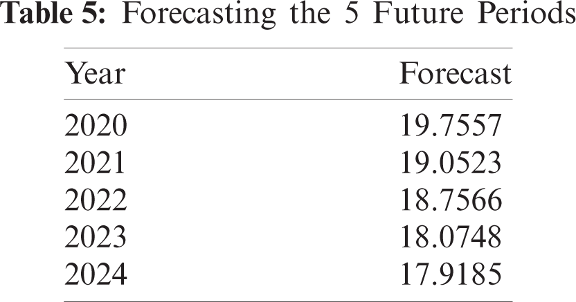
Based on the forecast results in Tab. 5, it can be seen that there is a decrease in the infant mortality rate from year to year. This result is in line with the opinion of Mishra et al. [10]; Kurniasih, et al. [19], and Hussein [20] who said that the infant mortality rate has decreased from year to year.

5  Conclusion and Impact

The purpose of this research is to model the infant mortality rate data and find the best model to predict this problem in the future. To achieve this goal, four model are used (ARIMA, Holt-Winters, Neural Network Time Series, and SutteARIMA) to predict the infant mortality rate data. To determine which prediction model is more suitable and precise in predicting data, the MAPE and MSE values of each of the forecasting methods used are calculated and the results are compared according to the predetermined performance criteria. Based on the findings of this study, it is concluded that the better or more suitable model, with smaller forecast errors in the infant mortality case data, is SutteARIMA which is then followed by Holt-Winters, ARIMA, and NNAR. And based on data trends and forecast results, the infant mortality rate is decreasing from year to year. The SutteARIMA method provides an estimated infant mortality rate for 2020 of 19.7557 and 17.9185 for 2024, a decline from 2019. These findings have the potential to help promote policies in order to address and minimize infant mortality rates in the coming years and can be used as a basis for implementing appropriate strategies to overcome them so that Indonesia's SDGs targets can be achieved. Although the infant mortality rate is predictable and has a satisfactory level of accuracy, it is possible that the results of this prediction are not precise due to human behavior and policies taken by policy makers.

Funding Statement: This research received funding from Taif University, Researchers Supporting and Project number (TURSP-2020/207), Taif University, Taif, Saudi Arabia.

Conflicts of Interest: The authors declare that they have no conflicts of interest to report regarding the present study.

References

 1.  U. Sivarajah, M. M. Kamal, Z. Irani and V. Weerakkody, “Critical analysis of Big data challenges and analytical methods,” Journal of Business Research, vol. 70, no. 1, pp. 263–286, 2017. [Google Scholar]

 2.  L. K. Grover and R. Mehra, “The lure of statistics in data mining,” Journal of Statistics Education, vol. 16, no. 1, pp. 1–9, 2008. [Google Scholar]

 3.  J. Edwards, In What is Predictive Analytics? Transforming Data into Future Insights, Singapore: CIO, 2019. [Online]. Available: https://www.cio.com/article/3273114/what-is-predictive-analytics-transforming-data-into-future-insights.html. [Google Scholar]

 4.  R. Bakri, U. Data and A. Saputra, “Marketing research: The application of auto sales forecasting software to optimize product marketing strategies,” Journal of Applied Science, Engineering, Technology, and Education, vol. 1, no. 1, pp. 6–12, 2019. [Google Scholar]

 5.  A. A. Ojugo and R. E. Yoro, “Predicting futures price and contract portfolios using the ARIMA model: A case of Nigeria's bonny light and forcados,” Quantitative Economics and Management Studies, vol. 1, no. 4, pp. 237–248, 2020. [Google Scholar]

 6.  S. I. Ranapurwala, J. E. Cavanaugh, T. Young, H. Wu, C. Peek-Asa et al., “Public health application of predictive modeling: An example from farm vehicle crashes,” Injury Epidemiology, vol. 6, no. 1, pp. 1–11, 2019. [Google Scholar]

 7.  M. A. El Safty, “Modeling uncertainty knowledge of the topological methods,” Poincare Journal of Analysis & Applications, vol. 8, no. 1(I), pp. 89–102, 2021. [Google Scholar]

 8.  M. A. El Safty and S. AlZahrani, “Topological modeling for symptom reduction of coronavirus,” Punjab University Journal of Mathematics, vol. 53, no. 3, pp. 47–59, 2021. [Google Scholar]

 9.  K. D. Jayanti, E. W. Wijaya, E. F. Bisono, R. F. Nurkhalim, I. Susilowati et al., “Proyeksi angka kematian bayi di rumah sakit X kabupaten kediri dengan single exponential smoothing,” Jurnal Berkala Kesehatan, vol. 6, no. 2, pp. 50–54, 2020. [Google Scholar]

10. A. K. Mishra, C. Sahanaa and M. Manikandan, “Forecasting Indian infant mortality rate: An application of autoregressive integrated moving average model,” Journal of Family & Community Medicine, vol. 26, no. 2, pp. 123–126, 2019. [Google Scholar]

11. D. A. Adeyinka and N. Muhajarine, “Time series prediction of under-five mortality rates for Nigeria: Comparative analysis of artificial neural networks, holt-winters exponential smoothing and autoregressive integrated moving average models,” BMC Medical Research Methodology, vol. 20, no. 1, pp. 1–11, 2020. [Google Scholar]

12. A. S. Ahmar and E. Boj, “The date predicted 200.000 cases of COVID-19 in Spain,” Journal of Applied Science, Engineering, Technology, and Education, vol. 2, no. 2, pp. 188–193, 2020. [Google Scholar]

13. A. S.Ahmar, S. Guritno and Abdurakhman, In Pendeteksian dan Pengoreksian Data Yang Mengandung Additive Outlier (AO) Pada Model ARIMA(p, d, q), Yogyakarta, ID: Gadjah Mada University, 2013. [Online]. Available: http://etd.repository.ugm.ac.id/home/detail_pencarian/59242. [Google Scholar]

14. W. W. S. Wei, “T ime Series Analysis: Univariate and Multivariate Methods,” 2nd ed., NY, USA: Pearson, 2006. [Google Scholar]

15. S. Lestari, A. S. Ahmar and R. Ruliana, “Eksplorasi metode triple exponential smoothing pada peramalan jumlah penggunaan air bersih di PDAM kota makassar,” VARIANSI: Journal of Statistics and Its Application on Teaching and Research, vol. 2, no. 3, pp. 128–146, 2020. [Google Scholar]

16. M. D. Wuryandari and I. Afrianto, “Perbandingan metode jaringan syaraf tiruan backpropagation dan learning vector quantization pada pengenalan wajah,” Jurnal Komputer dan Informatika (Komputa), vol. 1, no. 1, pp. 1–7, 2012. [Google Scholar]

17. A. S. Ahmar and E. Boj, “SutteARIMA: Short-term forecasting method, a case: Covid-19 and stock market in Spain,” Science of the Total Environment, vol. 729, no. 1, pp. 1–6, 2020. [Google Scholar]

18. A. S. Ahmar, “Forecast error calculation with mean squared error (MSE) and mean absolute percentage error (MAPE),” JINAV: Journal of Information and Visualization, vol. 1, no. 2, pp. 1–4, 2020. [Google Scholar]

19. N. Kurniasih, A. S. Ahmar, D. R. Hidayat, H. Agustin and E. Rizal, “Forecasting infant mortality rate for China: A comparison between α-sutte indicator, ARIMA, and holt-winters,” Journal of Physics: Conference Series, vol. 1028, no. 1, pp. 1–6, 2018. [Google Scholar]

20. M. A. Hussein, “Analysis and forecasting infant mortality rate (IMR) in Egypt until year 2000,” The Egyptian Population and Family Planning Review, vol. 25, no. 2, pp. 32–46, 1991. [Google Scholar]

This work is licensed under a Creative Commons Attribution 4.0 International License, which permits unrestricted use, distribution, and reproduction in any medium, provided the original work is properly cited.