Computers, Materials & Continua DOI:10.32604/cmc.2022.021300
Article

IoT-Cloud Empowered Aerial Scene Classification for Unmanned Aerial Vehicles

K. R. Uthayan1,*, G. Lakshmi Vara Prasad2, V. Mohan3, C. Bharatiraja4, Irina V. Pustokhina5, Denis A. Pustokhin6 and Vicente García Díaz7

1Department of Information Technology, Sri Sivasubramaniya Nadar College of Engineering, Chennai, 603110, India
2Department of Information Technology, QIS College of Engineering & Technology, Ongole, 523001, India
3Department of Electronics and Communications Engineering, Saranathan College of Engineering, Trichy, 620012, India
4Department of Electrical and Electronics Engineering, SRM Institute of Science and Technology, Chennai, 603203, India
5Department of Entrepreneurship and Logistics, Plekhanov Russian University of Economics, Moscow, 117997, Russia
6Department of Logistics, State University of Management, Moscow, 109542, Russia
7Department of Computer Science, University of Oviedo, Oviedo, 33003, Spain
*Corresponding Author: K. R. Uthayan. Email: uthayankr@ssn.edu.in
Received: 28 June 2021; Accepted: 29 July 2021

Abstract: Recent trends in communication technologies and unmanned aerial vehicles (UAVs) find its application in several areas such as healthcare, surveillance, transportation, etc. Besides, the integration of Internet of things (IoT) with cloud computing environment offers several benefits for the UAV communication. At the same time, aerial scene classification is one of the major research areas in UAV-enabled MEC systems. In UAV aerial imagery, efficient image representation is crucial for the purpose of scene classification. The existing scene classification techniques generate mid-level image features with limited representation capabilities that often end up in producing average results. Therefore, the current research work introduces a new DL-enabled aerial scene classification model for UAV-enabled MEC systems. The presented model enables the UAVs to capture aerial images which are then transmitted to MEC for further processing. Next, Capsule Network (CapsNet)-based feature extraction technique is applied to derive a set of useful feature vectors from the aerial image. It is important to have an appropriate hyperparameter tuning strategy, since manual parameter tuning of DL model tend to produce several configuration errors. In order to achieve this and to determine the hyperparameters of CapsNet model, Shuffled Shepherd Optimization (SSO) algorithm is implemented. Finally, Backpropagation Neural Network (BPNN) classification model is applied to determine the appropriate class labels of aerial images. The performance of SSO-CapsNet model was validated against two openly-accessible datasets namely, UC Merced (UCM) Land Use dataset and WHU-RS dataset. The proposed SSO-CapsNet model outperformed the existing state-of-the-art methods and achieved maximum accuracy of 0.983, precision of 0.985, recall of 0.982, and F-score of 0.983.

Keywords: Artificial intelligence; mobile edge computing; unmanned aerial vehicles; deep learning; optimization

1  Introduction

In recent days, Internet of Things (IoT) become a hot research topic and received huge attention among researchers to offer enormous services and applications. At the same time, the cloud computing (CC) technologies offer several benefits to support IoT applications and offer several benefits such as low latency, location aware, scalability, etc. [1]. At the same time, Unmanned Aerial Vehicle (UAV) technology has been significantly developed and used for many applications. UAVs can provide fast, cost-effective, and safe deployments for many civil and military applications [2]. Fig. 1 shows the architecture of Unmanned Aerial Vehicles (UAV).

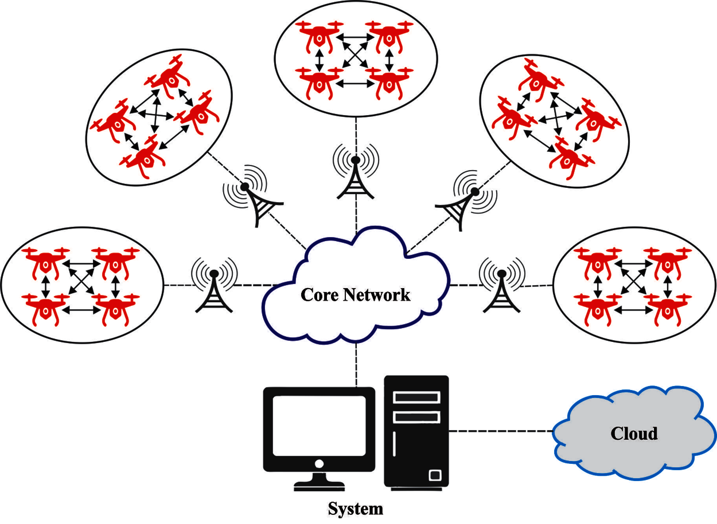
Figure 1: General structure of UAV networks

The popularity of independent UAVs and its applications, involving search and rescue operations, surveillance, and infrastructure observance in the recent years, is tremendous. Though land cover classification is an essential UAV application, it is complex to construct wholly-independent methods. Object identification processes are extremely integrated due to which it is difficult to reduce its cost demands. The movement of UAVs create multiple hindrances to the generated images in terms of clarity i.e., blurred images, and noise since the onboard cameras often generate low resolution images. In most of the UAV applications, it is difficult to perform the identification process because of the need for realistic efficiency. Various researches have been conducted on UAVs and its associated challenges such as tracking and detecting specific objects, types of vehicles, landmarks, land sites, and persons (involving pedestrian motion). But only a few studies considered multiple object identification [3] due to the fact that multiple targeted object identification is essential for most of the UAV applications. The occurrence of a break in application requirements and practical capability might be a result of two critical limitations: 1) it is difficult to build and store numerous methods to target the objects; and 2) high computation strength is required for technical object identification in case of individual objects.

When aerial image scenes are acquired, it undergoes aerial image classification. The images are categorized into sub-regions by covering several grounded objects and a variety of lands covering different semantic classes. Thus, aerial image classification is an important process for several real-world applications like computer cartography, urban planning, remote sensor, and resource management [4]. Generally, some of the identical object classes or land cover varieties are allocated in a pool of scenes. For example, commercial and residential are the two main classes of scenes which may include roads, buildings, and trees. However, these two classes have variances in spatial sharing and density of three class labels. Thus, in aerial scenes, classification is performed depending on structural and spatial pattern complications which is a challenging issue to overcome [5]. The common method is to construct a holistic scene demonstration for scene classification. Among the remote sensing studies, Bag of Visual Words (BoVW) is a familiar technique for scene classification. This technique was developed to investigate the text that implements a document via frequency of words. In order to identify the image via occurrences of ‘visual words’, local feature quantization is generated whereas BOW technique is utilized by clustering method. BoVW method is a form of BoW technique used for image analysis whereas all the images are determined as visual words from visual dictionary through the histogram of the former [6].

Deep Learning (DL) method [7] is highly beneficial in resolving conventional challenges such as object recognition and detection, Natural Language Processing (NLP), speech identification, and a number of such real-world applications. It is highly efficient than the usual processes and it also gained much attention in academia and industries. This technique attempts to acquire general hierarchical feature learning in terms of various abstract stages. UAV images are processed in real-time environment through two distinct ways namely, onboard processing of images with a GPU board and computation offloading through the transfer of DL algorithm processing from UAV to MEC. But there are several issues observed in the design of UAV-enabled MEC system.

The current research work presents an efficient DL-enabled aerial scene classification model for UAV-enabled MEC systems. The presented model allows the UAVs to capture aerial images and then forward the images to MEC for further processing. In addition, Capsule Network (CapsNet)-based feature extractor is applied to derive a set of useful feature vectors from the aerial image. Moreover, for hyperparameter optimization of CapsNet model, Shuffled Shepherd Optimization (SSO) algorithm is executed. Finally, Backpropagation Neural Network (BPNN) classification model is applied in the determination of appropriate class labels of aerial images. The presented SSO-CapsNet model was validated for its effectiveness against two openly accessible datasets.

2  Literature Review

Deep Convolutional Neural Network (CNN) [8] is one of the Deep Learning techniques which is familiar and gaining popularity in various identification and detection processes, since it produces optimum outcomes for regular datasets. In image classification, CNN achieves the highest accuracy and is the most preferred technique nowadays. For industrial usage, it is difficult to adjust the traditional Deep CNN (DCNN) due to the complications involved in fine tuning the hyperparameter manually and trade-off between computation cost and accurate classification. Several studies have attempted to reduce the computation cost incurred in its execution [9]. When using UAV aerial scene classification, the complication involved in traditional CNN gets reduced [10]. A particular type of CNN structure is chosen to decrease the search space and this lesser search space is made with the knowledge of experts.

Zhang et al. [11] utilized a so-called standard NN sparse autoencoder (AE) to train a group of chosen image patches and the model was tested by saliency degree to extract the local features. Coates et al. [12] improved the conventional Unsupervised Feature Learning (UFL) pipeline by feature learning. The acquaintance of CNN seems to be beneficial in various applications. In the study conducted by Lecun et al. [13], the CNN model was trained by backpropagation (BP) method and the study obtained adequate efficiency in character identification. In recent times, CNN is often utilized in computer vision research works. However, it is complicate to train deep CNN due to the possession of numerous features that are frequently utilized in particular process and the presence of low number of trained instances. The study was designed to extract the intermittent feature from DCNN. This model undergoes training on sufficiently large scale datasets such as ImageNet, that are utilized for a wider view of visible identification processes such as scene classification, object recognition, and image recovery.

Cimpoi et al. [14] achieved an optimum outcome when investigating the texture by pooling CNN features acquired from convolutional layer and fisher coding procedure. Research studies are still being conducted using CNN in UAV scene classification. In the literature [15], a pretrained CNN was employed and tuned completely on scene dataset demonstrating excellent classification outcome. But the pretrained CNN method was transferred to scene dataset due to the lack of trained models. In the study conducted earlier [16], the widespread possibility of CNN features, acquired from fully connected layer, underwent testing. In this study, the aerial images were categorized and the optimum outcomes were achieved over comparative techniques in open-source scene datasets. Although various techniques have been proposed for UAV image classification in the literature, there is a need exists to improve its class efficiency. Simultaneously, few techniques have provided optimum outcomes on specific datasets and were never employed on large datasets. Thus, the current research work develops a new advanced DL-based UAV image classifier.

3  The Proposed SSO-CapsNet Model

The working principle of the presented SSO-CapsNet model is illustrated in Fig. 2. As shown in the figure, UAV captures the aerial images which are then processed in MEC. The captured aerial images are then fed into CapsNet-based feature extractor to derive an effective set of feature vectors. Followed by, hyperparameter tuning of the CapsNet model is performed using the SSO algorithm. Finally, BPNN model is applied to allocate the class labels of the applied aerial test images. The detailed operations of these sub-processes are explained in the succeeding sections.

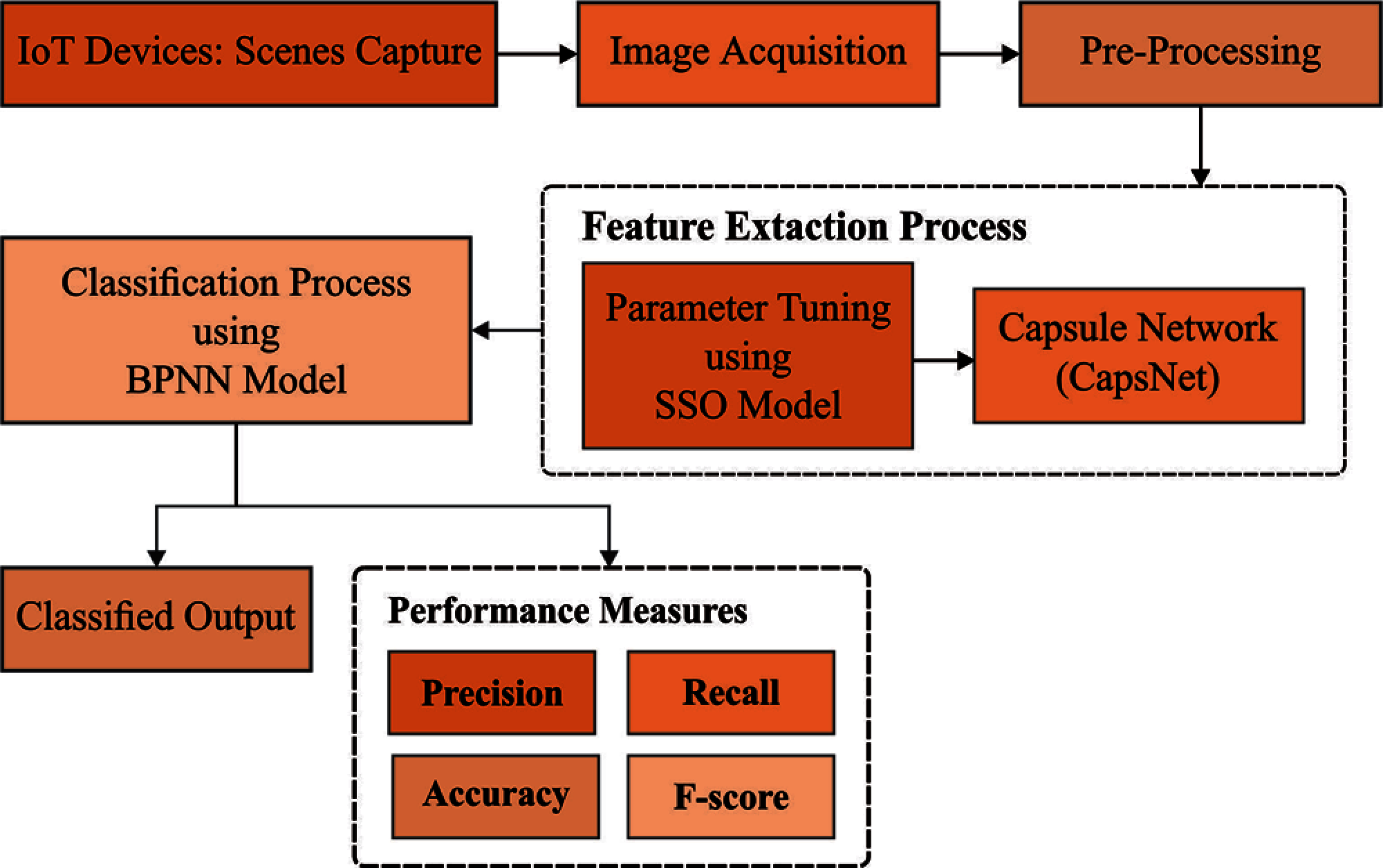
Figure 2: Working principle of SSO-CapsNet method

3.1 Capsule Network (Capsnet) Based Feature Extraction

CapsNets [17] is developed as an alternate model for CNNs. Being equivariant, the capsules are composed of a network of neurons that fetch in and yield out the vectors in line with scalar value of the CNNs. In CapsNet model, all the capsules are composed of a set of neurons with its output demonstrating various properties of similar features. It gives the benefit of identifying the entire set of entities through initial identification of their parts. Capsule outcome is made up of probability in which the feature encoder exists by capsules and the group of vector values is generally named after ‘instantiation parameters.’ It can be defined as the probability of existence of capsule's features to ensure network invariability. These instantiation parameters are utilized in the representation of network equivariance based on its capability for recognizing pose, texture, and deformation. Invariance is an asset of methods which makes the latter remain unchanged though the input value changes. This is called ‘translational invariance’ which is a peculiar characteristic of CNNs. For sample, when CNN detects the face, regardless of the position of eye, it stands still until it identifies the face. But, equivariance makes sure that the spatial position of features, proceeding to the face, is taken into account. Thus, in terms of outcome, equivariance does not consider the occurrence of an eye in image, but considers its position only in the image. Equivalences are the required properties for CapsNets.

The three commonly available operations for capsule execution are discussed here. They are transformation of AE, vector capsule depending on dynamic routing, and matrix capsule depending on Expectation-Maximization (EM) routing. Fig. 3 shows the structure of CapsNet model.

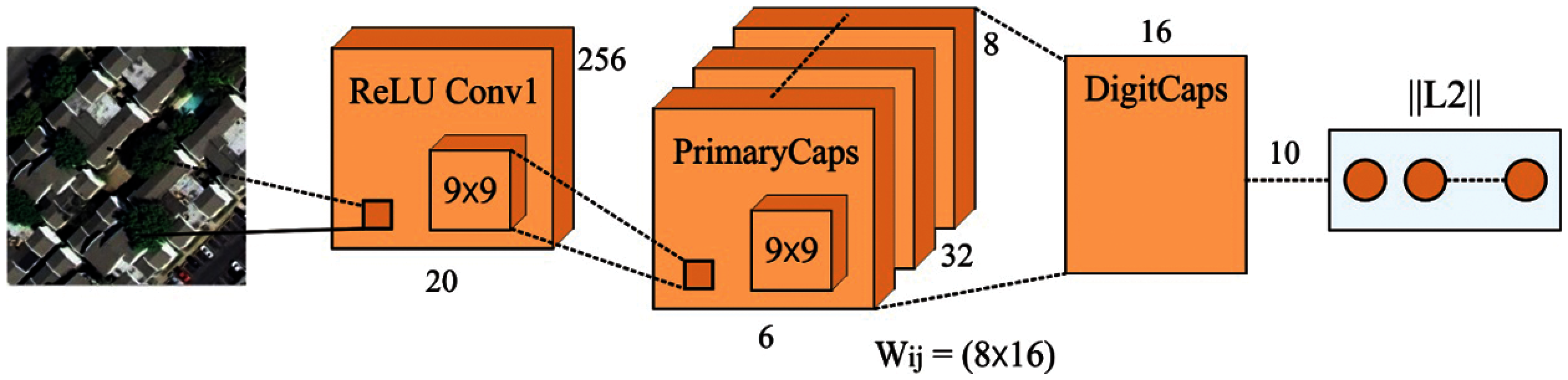
Figure 3: The architecture of CapsNet

3.1.1 Transformation of Auto-Encoders

An initial CapsNet is published with the transformation of AEs. It is constructed to emphasize the capability of network in recognizing the pose. The aim is not to identify an object from the images, but to take the image and their pose as input and output respectively, to form a similar image from original pose. An output vector of capsules, from this initial execution, is composed of output values. Further, one of the signified outcomes lies in these probabilities in which the feature exists through the rest of representative instantiating parameters. The capsules are ordered in various levels: the lower level l is named after initial capsule whereas the upper level l+1 is named after secondary capsule. Lower level capsule removes the ‘pose’ parameter in pixel intensities, since it has the ability to initiate a part-whole hierarchy [18]. This part-whole hierarchy is an advantage in CapsNets model since it identifies the parts and is developed to identify the whole set of entities too. In order to realize this, this feature is signified by lower level capsule which needs to have correct spatial connection. Previously, it activated higher-level capsules at level, l+1. For instance, assume that eyes and mouth are signified by lower level capsule. Then, each one can forecast to pose the higher-level capsules which signify a face in case of predictions being accepted. In order to describe the basis of initial-level capsule, ANN is learned to change the pixel intensity for pose parameter. In a simple method, 2D images, capsule by x and y with its positions, and its only pose output are utilized. Once the learning process is over, the network takes an image and there is a need arise to shift Δx and Δy. Then the output of an image remains the identified shift in pose. In order to prevent the influence of inactive capsule from affecting the output of ‘generation unit,’ the capsule output is multiplied by probabilities, p.

3.1.2 Dynamic Routing Between Capsules

The next level of changes in CapsNets is determined by the capsules which are nothing but a set of neurons with instantiation parameter. These changes are even signified by activity vector, whereas the length of vector signifies the probability in which the feature exists. The enhancement with a detailed prior execution exhibits that there is no need of information in the input [19]. The networks are composed of three layers namely, Convolutional (Conv) layer, Primary Capsule (PC) layer, and Class capsule layer. PC layer is the initial capsule layer which is only next to undetermined number of capsules’ layer. The final capsules’ layer is named after Class capsules layer. Feature extraction process from an image is completed by Conv. layer and the output is fed to PC layer. In all the capsules, i (where 1≤i≤N) in layer l takes the activity vector ui∈R into account for encoding spatial data in the procedure of instantiation parameter. The output vector ui of ith lower-level capsules are then fed to every capsule from next layer, l+1. The jth capsule at layer l+1 is obtained i.e., ui and their product is defined with equivalent weight matrix i.e., Wij. The resultant vector u^j∣i is the capsule i at level l's change of entities which is signified by capsule j at level l+1. In the prediction vector of PC, u^j∣i refers to PC whereas i corresponds to the class capsule, j.

u^j∣i=Wijui(1)

The product of prediction vectors and coupling coefficient, which together signifies the agreement between the capsules, is performed to obtain a single PC i's forecast for class capsule, j. When the agreement is higher, both the capsules are related together. Thus, in the outcome, the coupling coefficient is first increased which is then decreased. The weighted sum (sj) of every individual PC forecasts to the class capsule, j is computed to achieve the candidates’ squashed function, (vj).

sj=∑i=1N⁡ciju^j∣i(2)

cij=exp(bij)∑k⁡exp⁡(bik)(3)

The squashed function makes sure that the length of output in capsules lies between 0 and 1 as probability. vj in one capsule layer is sent to next layer capsules and processed in a similar manner. The coupling coefficient cij makes sure that the forecast of i in level l is connected to j in layer l+1. In all the iterations, cij is upgraded by determining the dot product of u^j∣i and vj. To be specific, the vector values connected to all capsules are observed as mere segments of two numbers; the probabilities signify the presence of feature which the capsules tend to encapsulate and a group of instantiation parameters that assist in the clarification of consistency among the layers. Thus, a related path by agreement stems in detail that if lower-level capsule decides the higher level layer capsules, it is ‘construct a part whole’ connection referring to the relevance of path.

3.1.3 Matrix Capsules with EM Routing

On the contrary to utilization of vector outputs, the literature [20] presented the illustration of input and output of capsule as matrices. It is essential to decrease the size of transformation matrices between capsule and matrix. Further, it is developed by n elements rather than n2 when utilizing vectors. Dynamic routing by agreement is exchanged with EM technique. This dynamic routing is cosine between two pose vectors. Also, the probability of existence of entity, even illustrated by capsule, is exchanged with a parameter a, rather than the length of vectors. In the capsule i at level L and capsule j at level L+1, these values refer to the trainable transformation weight matrix i.e., Wij. EM mechanism ensures that the shift matrix of capsule i is changed by transformation weight matrix Wij to cast the vote to shift the matrix of capsule, j at level L+1. Vote is an artefact of output matrix Mi and transformation matrix Wij [20].

Vij=MiWij(4)

The poses and activations of every L+1 level layer are established by entering Vij and ai as non-linear EM routing techniques. During an iteration, EM upgrades the means, variances, and activation probabilities of layer L+1 capsules with the assignment probability between lower and higher level capsules.

3.2 Hyperparameter Optimization

In order to tune the hyperparameters involved in CapsNet model effectively, SSO algorithm is applied and thereby the classification performance is enhanced. SSO algorithm offers several benefits such as maximum accuracy, convergence rate, and reduced parameter dependency. It is based on the herd performance of shepherds. Humans have to learn this phenomenon through long-term observation so as to utilize animal capabilities and attain the objectives [21]. Shepherds try to steer their herd in a right way. To resolve this, they generally set animals such as horse or herding dog for the herd. These animals are utilized to manage the herd through their herding behaviour. They further guard the herd animals from wild animals and theft. This performance is the fundamental information to follow the SSO technique.

Step 1: Initialization

SSO begins with an arbitrarily-created primary Member Of Community (MOC) for search space as given herewith.

i=1,2,…,mandj=1,2,…,n(5)

where rand refers to arbitrary vector by all components created between 0 and 1; Here, MOCmin and MOCmax denote the lower and upper bounds of design variables; m implies the amount of communities, and n defines the count of members going to all the communities. In this regard, it is supposed that the entire number of communities is attained as [21] follows.

nMC=m×n(6)

Step 2: Shuffling process

In this method, initial m refers to the members of communities which are chosen depending on their objective function values. These are arbitrarily located values in the first column of Multi-Community (MC) matrix (Eq. (7)) which are otherwise, the initial member of all the communities. Then, to create the 2nd column of MC, next m members are selected alike the preceding step which are arbitrarily located in the column. These procedures are carried out for n times independently, until the MC matrix gets molded as given herewith.

MC=[MOC1,1MOC1,2⋯MOC1,j⋯MOC1,nMOC2,1MOC2,2⋯MOCi,j⋯MOC2,n⋮⋮⋮⋮⋮⋮MOCi,1MOCi,2⋯MOCi,j⋯MOCi,n⋮⋮⋮⋮⋮⋮MOCm,1MOCm,2⋯MOCm,j⋯MOCm,n](7)

It is worth mentioning that all the rows of MC refer to the members of all the communities. This phenomenon ensures that the members of initial column of MC are optimal members, compared to all other communities. Moreover, the member's place in final column is the bad agent in all communities.

Step 3: Movement of Community Member

The unique step size of the movement in all the communities is calculated depending on two vectors. Initial vector (i.e., stepsizei,jWorse) showcases the capability to visit new regions of search space (diversification approach). In contrast, the 2nd vector (i.e., stepsizei,jBetter) refers to the ability of exploring those search space areas (intensification method) which are nearby and already visited. The mathematical equation for step size is given herewith [21]:

i=1,2,…,mandj=1,2,…,n(8)

where stepsizei,jWorse and stepsizei,jBetter are determined as follows:

stepsizei,jWorse=α×rand1×(MOCi,w−MOCi,j)(9)

stepsizei,jBetter=β×rand2×(MOCi,b−MOCi,j)(10)

where rand1 and rand2 represent the arbitrary vectors with all the even components created between 0 and 1; MOCi,b(chosen horses) and MOCi,w(chosen sheep's) are optimal and worst members with respect to objective function value and is related to MOCi,j(shepherd). It is worth to mention that the initial member of ith community (MOCi,1) mostly prefer itself rather than considering other members. So, stepsizei,1Better is equivalent to zero. Conversely, MOCi,n doesn't take the member worst itself, since it has to ensure the final member of ith community i.e., stepsizei,1Worse is equivalent to zero. Furthermore, α and β imply the factors which control exploration as well as exploitation correspondingly. These aspects are determined as follows.

α=α0−α0×t;t=iterationMaxiteration(11)

β=β0+(βmax−β0)×t(12)

It is obvious that the iteration number t and β increase whereas α value decreases correspondingly. Thus the outcome and exploration rate decreases whereas the exploitation rate increases [22].

Step 4: Update the position of each community member

Based on the prior step, the new location of MOCi,j is computed utilizing Eq. (13). Next, the location of MOCi,j is upgraded, when it could not find the worst old objective function value [22]:

newMOCi,j=MOCi,j+stepsizei,j(13)

Step 5: Checking termination conditions

Later, the count of iterations is set as the end condition (Max-iteration), then the optimization procedure is finished. Afterwards, it goes to step 2 for a new round of iteration.

3.3 BPNN Based Image Classification

At the final stage, the extracted feature vectors from hyperparameter-tuned CapsNet are fed into BPNN model to perform the classification. BPNN is a multi-layer network which has a set of input, hidden, and output layers. All the layers contain a number of neurons. To adjust the weight and bias in neurons, BPNN uses error BP function. It is beneficial in a gradient-descent feature and this technique is developed as an efficient function estimate technique [23]. Classical BPNN has a number of m inputs and n outputs.

In feedforward network, all the neurons from the next layer act as input in every neuron for the outputs from final layer. Afterwards, the output is fed as input for the next neuron layer. In one neuron j, assume n refers to the number of neurons in final layer; oi refers to the output of ith neuron; wi represents the equivalent weight for oi and θj implies the bias of neurons j. Then, the neurons j compute the input for sigmoid function, Ij utilizing the equation [23].

Ij=∑n⁡wioi+θj(14)

Assume oj indicates the output of neuron, j which is expressed as follows

oj=1(1+e−Ij)(15)

When the neuron j implies the output layer, BPNN begins the BP level. Assume tj refers to encoder target output. This technique calculates the output error Errj to neuron j in the output layer with the help of following equation.

Errj=oj(1−oj)(tj−oj)(16)

Assume k signifies the amount of neurons in next layer; wp refers to weight; and Errp defines the neuron error, p in next layer. The error Errj of jth neurons is expressed as follows

Errj=oj(1−oj)∑k⁡Errpwp(17)

Assume η indicates the rate of learning. Neuron j tunes its weight wj and bias θj with the help of [23].

Δθj=ηErrj,(18)

If BPNN finishes tuning the network by one trained sample, it begins with a second trained sample with the output of first trained sample as an input to train the second sample. For executing the classifier, BPNN requires only the execution of the feedforward network. The outputs at the output layer are the final classifier outcome.

4  Experimental Validation

The proposed SSO-CapsNet model was simulated using Python 3.6.5 tool. It was validated using two datasets namely, UCM and WHU-RS datasets. UCM dataset is composed of a large-sized aerial image under 21 classes. Every class holds a total of 100 images with an identical size of 256*256 pixels. WHU-RS dataset includes a total of 950 images with an identical size of 600*600 pixels. These images undergo uniform distribution under a set of 19 classes. Few sample test images are shown in Fig. 4.

Tab. 1 and Fig. 5 show the results of accuracy analysis attained by SSO-CapsNet model against different CNN models. The table values report that the PlacesNet model obtained the least accuracy of 0.914. Simultaneously, the VGG-VD19 technique exhibited a slightly higher accuracy of 0.932, whereas the VGG-VD16 model achieved an improved accuracy of 0.941. Concurrently, AlexNet, CaffeNet, and VGG-F methods accomplished a reasonable and same accuracy of 0.944. In line with these, VGG-M model demonstrated improvement over the earlier models and achieved an accuracy of 0.945. Meanwhile, the VGG-S model showcased a reasonable accuracy of 0.946. However, the presented SSO-CapsNet model surpassed other methods and attained a maximum accuracy of 0.983.

Tab. 2 and Fig. 6 examine the performance of SSO-CapsNet model against the existing models in terms of different measures. When analyzing the results in terms of F-score, the table values show that the VGGNet model obtained the least F-score of 0.785. Likewise, the VGG-RBFNN model exhibited a slightly increased F-score of 0.788 whereas the CA-VGG-LSTM model accomplished a certain improvement in F-score i.e., 0.796. Followed by, ResNet-50 model depicted a manageable outcome with an F-score of 0.797 while the CA-VGG-BiLSTM model resulted in an F-score of 0.798. Simultaneously, ResNet-RBFNN model achieved a reasonable F-score of 0.806. Concurrently, GNet model accomplished an F-score of 0.807, whereas an even higher F-score of 0.814 was offered by CA-ResNet-LSTM model. In line with this, GoogLeNet-RBFNN model demonstrated an improvement in the results over earlier models with an F-score of 0.815 and the CA-ResNet-BiLSTM model provided an F-score of 0.815. Meanwhile, CA-GNet-LSTM model attempted to showcase a reasonable F-score of 0.818, whereas CA-GNet-BiLSTM model accomplished a competitive F-score of 0.818. However, the presented SSO-CapsNet model surpassed all other methods and achieved a high F-score of 0.983.

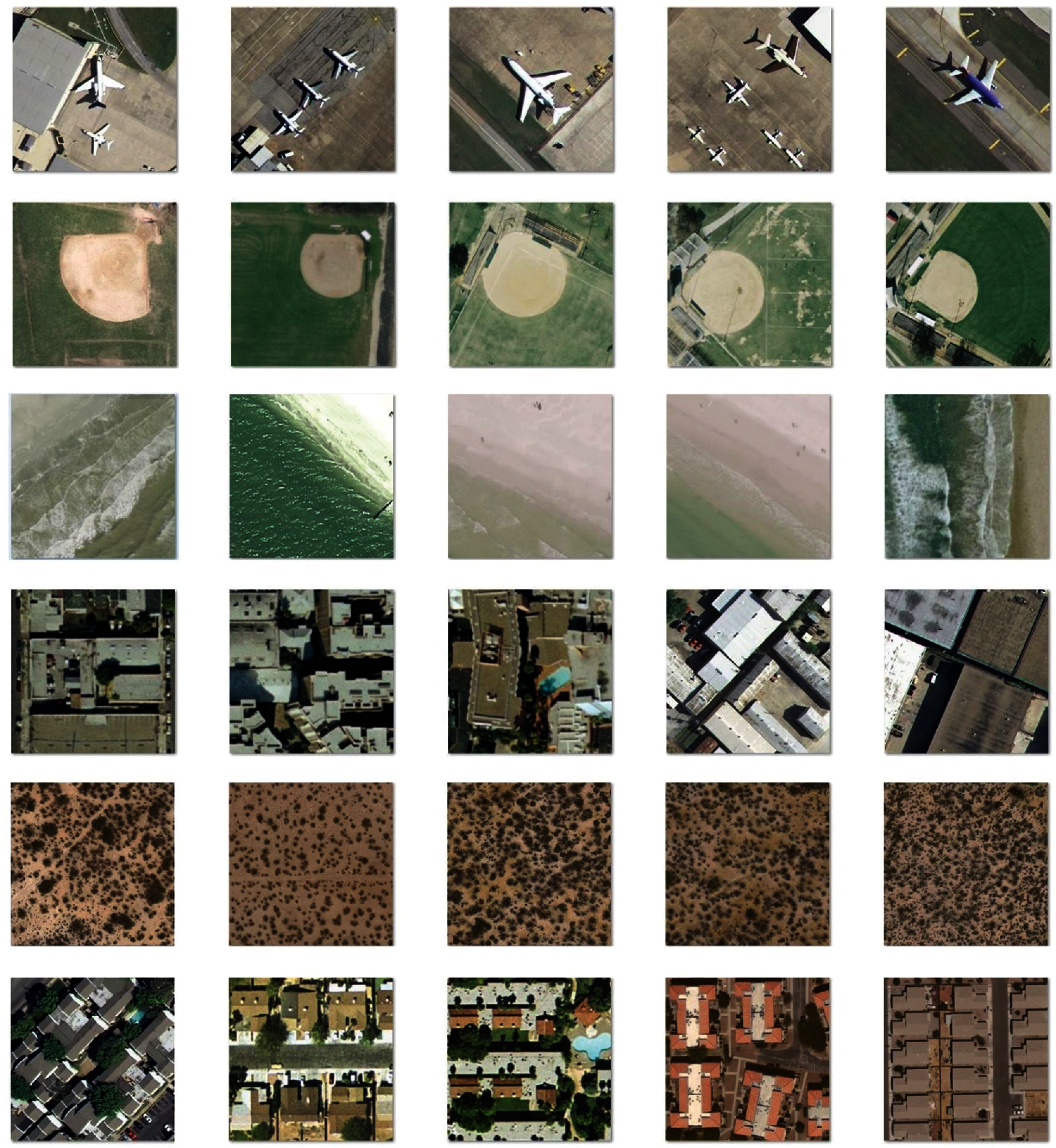
Figure 4: Sample images

When investigating the outcomes with respect to precision and recall, the table values portray that the CA-ResNet-BiLSTM model obtained the least precision and recall values such as 0.779 and 0.890 respectively. At the same time, VGG-RBFNN approach exhibited slightly higher precision and recall values i.e., 0.782 and 0.839 respectively, whereas the CA-GNet-LSTM model reached superior precision and recall values such as 0.785 and 0.886 respectively. Followed by, VGGNet model depicted a manageable outcome while its precision and recall values were 0.791 and 0.823 respectively. Further, CA-VGG-BiLSTM yielded the following precision and recall values i.e., 0.793 and 0.840 respectively. Simultaneously, the ResNet-RBFNN model achieved a reasonable precision and recall of 0.799 and 0.846 correspondingly. Concurrently, CA-ResNet-LSTM model accomplished a precision and recall of 0.799 and 0.861 correspondingly. A further increase was observed in precision and recall values such as 0.799 and 0.871 by CA-GNet-BiLSTM model. Followed by, the GoogLeNet-RBFNN model demonstrated an improved outcome over earlier models with a precision and recall of 0.800 and 0.868 correspondingly. The GNet method attained 0.805 precision and 0.843 recall value. Meanwhile, the CA-VGG-LSTM model demonstrated reasonable precision and recall values such as 0.806 and 0.825 respectively. Further, ResNet-50 method resulted in competitive precision and recall values i.e., 0.809 and 0.820 respectively. However, the proposed SSO-CapsNet technique surpassed all other methods and offered the highest precision and recall values such as 0.985 and 0.982.

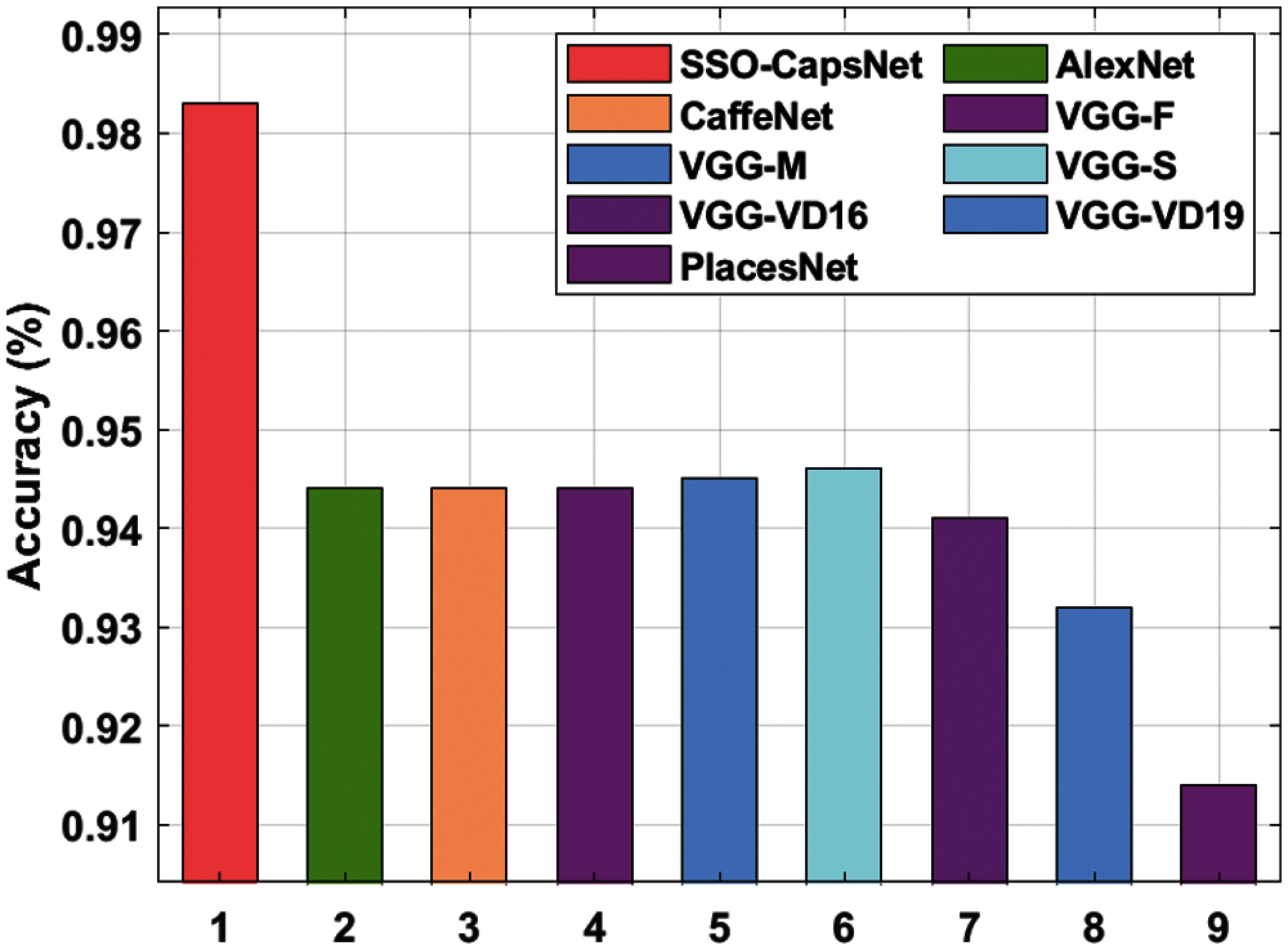
Figure 5: Accuracy analysis of SSO-CapsNet model with distinct CNN models

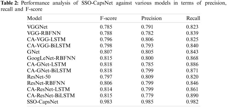
Figure 6: Result of SSO-CapsNet Model under distinct measures

Tab. 3 and Fig. 7 portray the results of accuracy analysis conducted upon SSO-CapsNet model against the existing models. The table values infer that the SCK model achieved a minimum accuracy of 0.725. At the same time, SPM model exhibited a slightly increase in accuracy up to 0.740, whereas SPCK++ model accomplished a higher accuracy of 0.774. Followed by, SC+Pooling model depicted a manageable outcome with an accuracy of 0.817. Likewise, SG+UFL and CCM-BOVW models accomplished similar results i.e., accuracy of 0.866. Simultaneously, PSR model achieved a reasonable accuracy of 0.891. Concurrently, UFL-SC model accomplished an accuracy of 0.903, whereas an enhanced accuracy of 0.909 was attained by OverFeat model.

In line this these, MSIFT and COPD models exhibited higher outcomes over earlier models and its accuracy values were 0.910 and 0.913 respectively. The Dirichlet model provided moderate results with an accuracy of 0.928. Meanwhile, VLAT and GoogLeNet+Finetune models showcased reasonable accuracy values such as 0.943 and 0.971 correspondingly. The CCP-Net and MOPSO-SC methodologies provided competitive accuracies such as 0.975 and 0.979 respectively. However, the presented SSO-CapsNet model surpassed all other models and accomplished a superior accuracy of 0.983.

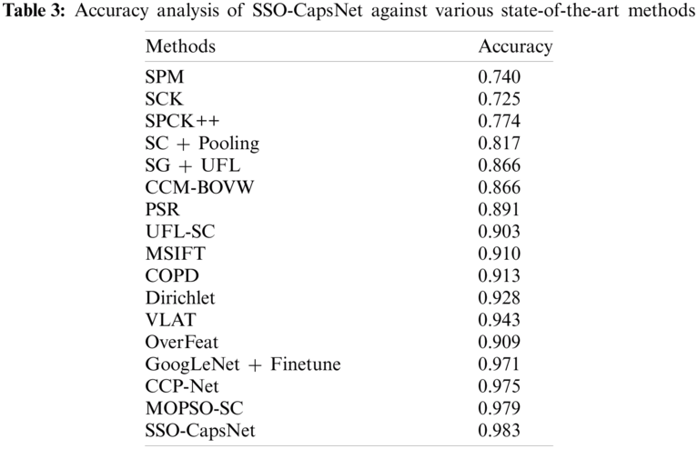
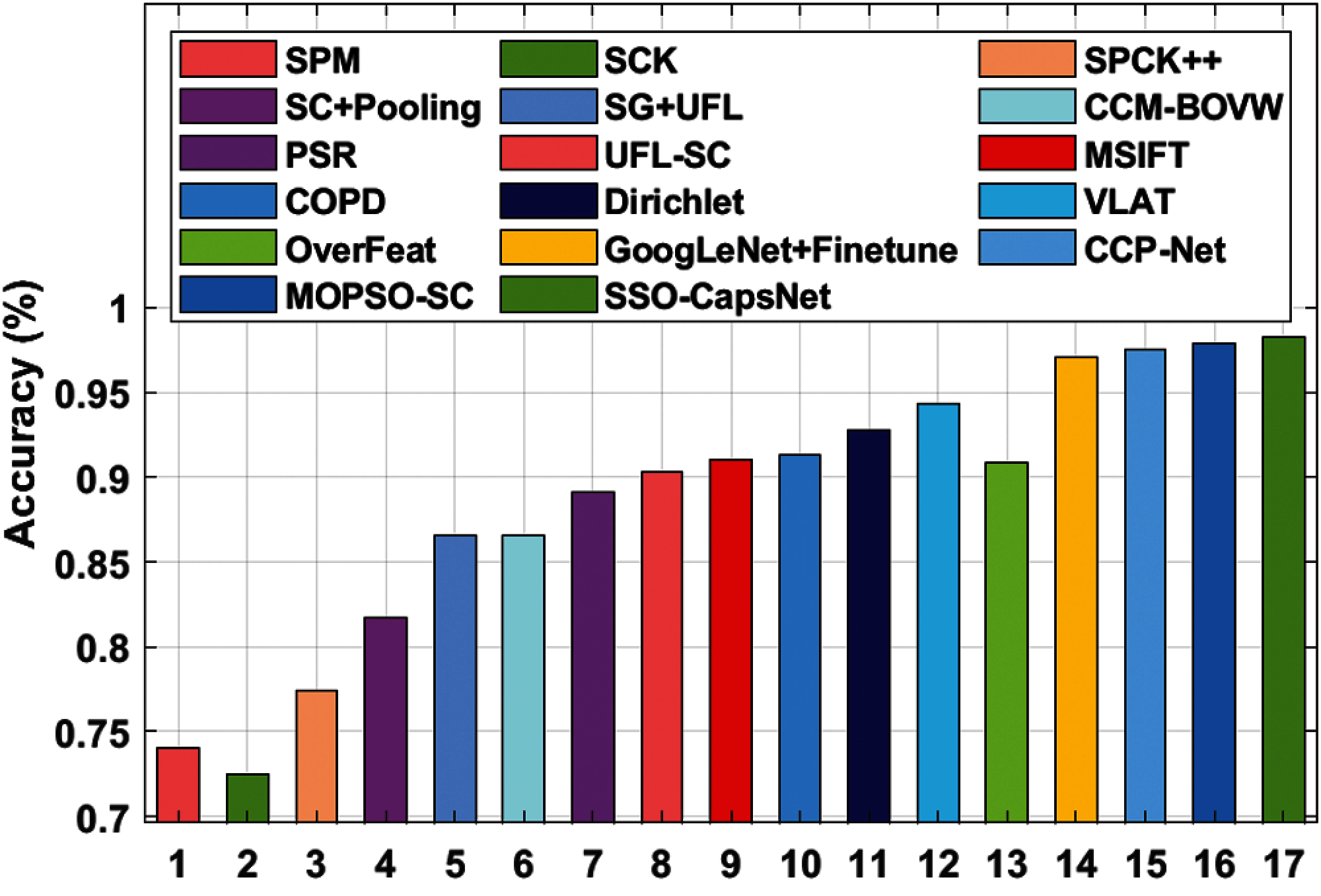
Figure 7: Accuracy analysis of SSO-CapsNet model against existing techniques

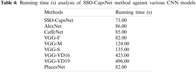
Tab. 4 illustrate the results for running time analysis of SSO-CapsNet model against other CNN models [5,24–26]. The results portray that both VGG-16 and VGG-19 models demonstrated the worst performance and achieved high running time of 423 and 496 s respectively. In line with these, VGG-M and VGG-S models demonstrated slightly enhanced results with respective running times being 124 and 135 s. Followed by, CaffeNet and AlexNet models reported moderate running time of 85 and 86 s respectively. Moreover, PlacesNet and VGG-F models showcased somewhat reasonable and same running time of 82 s. But the SSO-CapsNet model displayed superior performance and accomplished the task at a running time of 73 s.

5  Conclusion

The current study developed a new DL-enabled aerial scene classification model for UAV-enabled MEC systems i.e., SSO-CapsNet model. The presented model allows the UAVs to capture aerial images and send it to MEC for further processing. At MEC, the captured aerial images are fed into CapsNet-based feature extractor to derive an effective set of feature vectors. Followed by, SSO algorithm is used to fine tune the hyperparameters of CapsNet model. The application of SSO algorithm helps in effectively tuning the hyperparameters. Thus, the accuracy of overall aerial image scene classification is enhanced. Finally, BPNN model is applied to allocate the class labels of the applied aerial test images. The simulation results of the proposed SSO-CapsNet model were validated against the benchmark UCM and WHU-RS datasets. The obtained experimental values inferred that the SSO-CapsNet model outperformed other classifiers and accomplished the maximum accuracy of 0.983, precision of 0.985, recall of 0.982, and F-score of 0.983. In future, SSO-CapsNet model can be implemented in handling various input sizes with multiple scaling. Further, the model can be assessed on big datasets such as NWPU-resic45 for its performance.

Funding Statement: The authors received no specific funding for this study.

Conflicts of Interest: The authors declare that they have no conflicts of interest to report regarding the present study.

This work is licensed under a Creative Commons Attribution 4.0 International License, which permits unrestricted use, distribution, and reproduction in any medium, provided the original work is properly cited.