DOI:10.32604/cmc.2022.021113
| Computers, Materials & Continua DOI:10.32604/cmc.2022.021113 | |
| Article |
A Hybrid Deep Learning-Based Unsupervised Anomaly Detection in High Dimensional Data
1Department of Computer and Information Sciences, Universiti Teknologi PETRONAS, Seri Iskandar, 32160, Malaysia
2Centre for Research in Data Science (CERDAS), Universiti Teknologi PETRONAS, Seri Iskandar, 32610, Perak, Malaysia
3Information Systems Department, Prince Sultan University, Riyadh, 11586, Saudi Arabia
*Corresponding Author: Amgad Muneer. Email: amgad_20001929@utp.edu.my
Received: 22 June 2021; Accepted: 23 July 2021
Abstract: Anomaly detection in high dimensional data is a critical research issue with serious implication in the real-world problems. Many issues in this field still unsolved, so several modern anomaly detection methods struggle to maintain adequate accuracy due to the highly descriptive nature of big data. Such a phenomenon is referred to as the “curse of dimensionality” that affects traditional techniques in terms of both accuracy and performance. Thus, this research proposed a hybrid model based on Deep Autoencoder Neural Network (DANN) with five layers to reduce the difference between the input and output. The proposed model was applied to a real-world gas turbine (GT) dataset that contains 87620 columns and 56 rows. During the experiment, two issues have been investigated and solved to enhance the results. The first is the dataset class imbalance, which solved using SMOTE technique. The second issue is the poor performance, which can be solved using one of the optimization algorithms. Several optimization algorithms have been investigated and tested, including stochastic gradient descent (SGD), RMSprop, Adam and Adamax. However, Adamax optimization algorithm showed the best results when employed to train the DANN model. The experimental results show that our proposed model can detect the anomalies by efficiently reducing the high dimensionality of dataset with accuracy of 99.40%, F1-score of 0.9649, Area Under the Curve (AUC) rate of 0.9649, and a minimal loss function during the hybrid model training.
Keywords: Anomaly detection; outlier detection; unsupervised learning; autoencoder; deep learning; hybrid model
Nowadays, a huge amount of data is produced periodically at an unparalleled speed from diverse and composite origins such as social media, sensors, telecommunication, financial transactions, etc. [1,2]. Such acceleration in data generation yields to the concept of big data, which can be attributed to the umpteen and dynamism in technological advancements. For instance, the emergence of the Internet of Things (IoT) and the increase in smart devices usages (wearables and non-wearables) have contributed to the upsurge in the continuous generation of data [3]. As defined by Gandomi et al. [4], big data can be described as high-volume, high-velocity, and high-variety datasets where knowledge or insights can be derived using data analytic tools. Moreover, big data is conceptualized as the 5 Vs (Value, Veracity, Variety, Velocity and Volume) [5]. As shown in Fig. 1, Value depicts the advantage of data analysis; veracity shows the level of accuracy while Variety represents the different kinds of data (structured, semi-structured, and unstructured) present in big data [6]. Concerning Volume, it shows the magnitude of data being processed or stored. However, an increment in the volume of data leads to an increase in the dimensionality of such data. Dimensionality is the number of features or attributes present in each dataset. On the other hand, Velocity represents the rate at which data are produced which may consist of several dimensions. The preceding statements showed how the 5 Vs of big data addresses its underlining limitations [7]. Nonetheless, the dimensionality of data, which is proportional to the volume of the data is somewhat overlooked. Increment or large dimensions of data could negatively affect the extraction of knowledge from a dataset. That is, high dimensionality can affect data analytics such as anomaly detection in a large dataset.
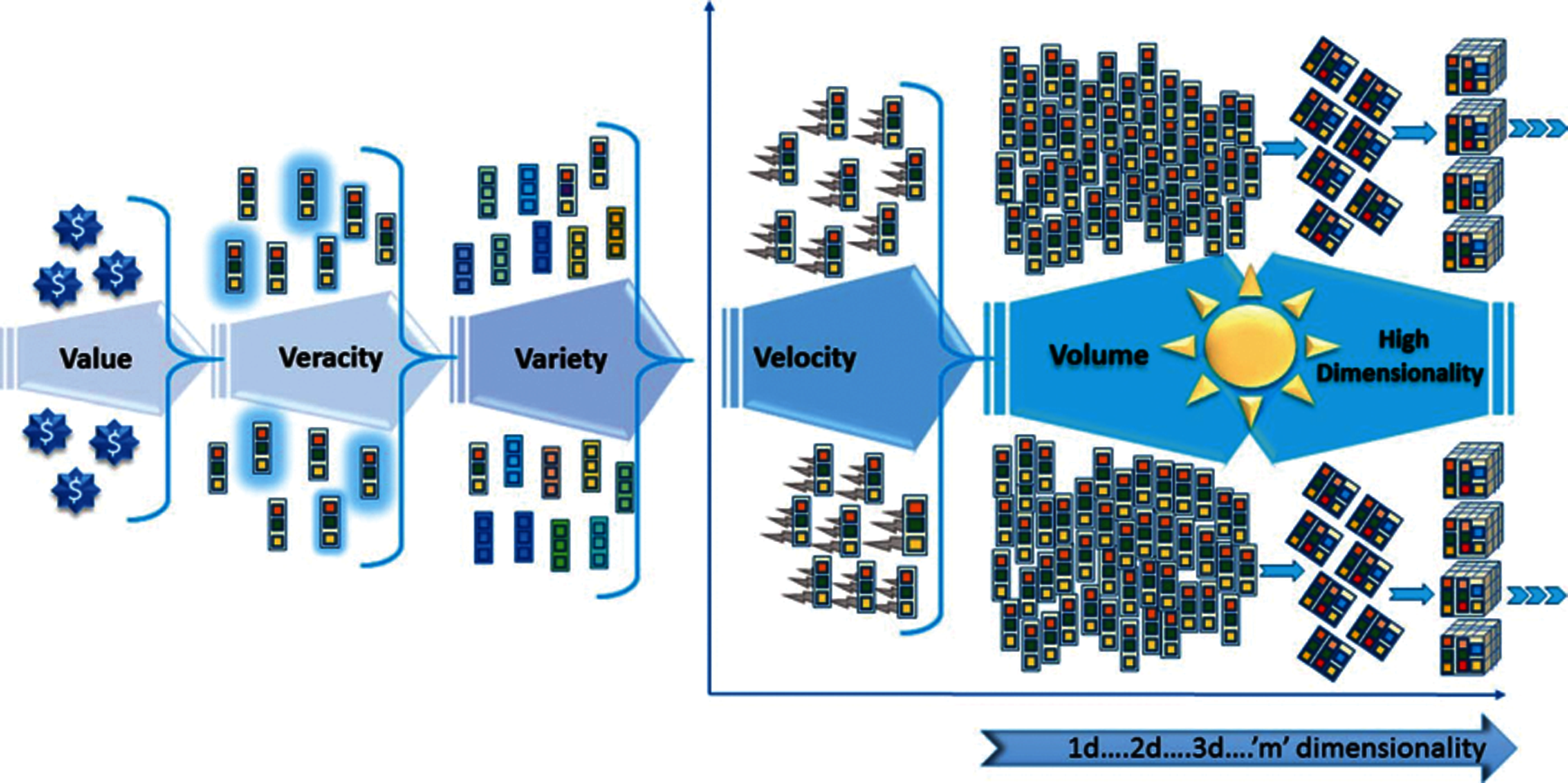
Figure 1: High dimensionality problem in big data [5]
Anomaly detection points to the challenge of detecting trends in data that do not correspond to anticipated behavior [8]. In various implementation domains, these non-conforming patterns are referred to as deviations, outliers, discordant observations, variations, aberrations, shocks, peculiarities, or pollutants [9,10]. The existence of anomalies in each dataset can be seen as a data quality problem as it can lead to undesired outcomes if not removed [11,12]. As such, the removal of anomalous points from a dataset leads to data quality improvement, which makes the given dataset an imperative [13]. Besides, closeness of the data objects to one another yields to the high dimensionality in datasets, which will lead to the ambiguity in the respective data distances [14]. Although there are several detection techniques which require sophisticated and efficient computational approaches [8,15], the conventional anomaly detection techniques cannot adequately handle or address the high-dimensionality issue. Besides, many of these conventional anomaly detection techniques infer that the data have uniform attributes or features. On the contrary, real-life datasets in most cases have diverse types of attributes. This observation points to a heightened problem in anomaly detection [5,8,15].
Several anomaly detection techniques have been proposed across different application domains [14–18]. Neighbor-based anomaly techniques such as LOF, kNNW, ODIN detects anomalies using neighborhood information from data points [19–21]. These methods record poor performance and are somewhat conscious of the parameters of proposed methods. Another instance is the recent ensemble-based anomaly detection techniques. Zimek et al. [22] and Pasillas-Díaz et al. [23] proposed an ensemble-based anomaly detection method with good performance. However, ensemble methods are a black-box mechanism that lacks explain ability. Besides, selecting the most applicable and appropriate meta-learner is an open research problem. Another example, Wilkinson [24] proposed an unsupervised algorithm known as HDoutliers that can detect anomalies in high-dimensional datasets. Findings from the comparative study by Talagala et al. [25] also corroborate the efficiency of the HDoutliers algorithm. However, the tendency of HDoutliers to increase the false negatives rate is its drawback. Chalapathy et al. [26], Wu et al. [27], and Favarelli et al. [28], in their respective studies, proposed One-Class Neural Network anomaly detection methods for small and large-scale datasets. Also, Malhotra et al. [29], Nguyen et al. [30], Zhou et al. [17], and Said Elsayed et al. [31] developed anomaly detection methods based on long short-term memory (LSTM). However, these existing methods cannot handle the class imbalance problem.
Instigated by the preceding problems, this study proposes a novel hybrid deep learning-based approach for anomaly detection in large-scale datasets. Specifically, a data sampling method and multi-layer deep autoencoder with Adamax optimization algorithm is proposed. Synthetic Minority Over-sampling Technique (SMOTE) is used as a data sampling method to resolve the inherent class imbalance problem by augmenting the number of minority class instances to the level of the majority class label. A novel deep autoencoder neural network (DANN) with Adamax optimization algorithm is used for detecting anomaly and reducing dimensionality. The primary contributions of this work are summarized as thus:
• A novel DANN approach to detect anomalies in time series by the unsupervised mode.
• Hybridization of SMOTE data sampling and DANN to overcome inherent class imbalance problem.
• We addressed and overcame the curse of dimensionality in data by applying a multilayer autoencoder model that can find optimal parameter values and minimize the difference between the input and the output using deep reconstruction error during the model training.
The rest of this paper is structured as follows. Section 2 highlighted the background and the related works of the study. Section 3 outlines this work's research methodology, while Section 4 describes the experimental findings. Lastly, Section 5 concludes the paper and highlights the future work.
Anomaly detection is a well-known issue in a variety of fields, so different approaches have been proposed to mitigate this issue recently. Further information about this issue can be found in [5,32–35]. In this section, we will look at some of the more common anomaly detection techniques, and the relevant enhancements.
One of the commonly used anomaly detection technique is called neighbor-based anomaly detection technique whereby the outliers are identified based on the neighborhood information. Thus, the anomaly is scored as the average or weighted distance between the data object and its k nearest neighbors [19,21]. Another option is using the local outlier factor (LOF) to determine the anomaly degree whereby the anomaly score is calculated in accordance with its neighborhood [36]. Likewise, Hautamaki et al. [20] proposed an Outlier Detection using Indegree Number (ODIN), which is based on kNN graph, whereby data instances are segregated based on their respective influence in its neighborhood. It is worth mentioning that all the above-mentioned neighbor-based detection methods are independent of data distributions and can detect isolated entities. However, their success is heavily reliant on distance scales, which is unreliable or insignificant in the high-dimensional spaces. Thus, considering the ranking of neighbors is a viable solution to overcome this issue as the existence of high-dimensional data still makes the ranking of each object's nearest neighbors significant. The underlying assumption is that if the same process created two objects, they would most likely become nearest neighbors or have similar neighbors [37].
Another applicable approach is deploying the subspace learning method. Sub-space-based anomaly detection approaches try to locate anomalies by sifting through various subsets of dimensions in an orderly manner. According to Zimek et al. [22], only a subset of relevant features for an object in a high dimensional space provides useful information, while the rest are unrelated to the mission. The presence of irrelevant features can make the anomaly detection process challenging to distinct. Another direction is using sparse subspace technique, which is a kind of subspace technique. Both points in a high-dimensional space are projected onto one or more low-dimensional, called sparse subspaces in this case [38,39]. As a result, objects that collapse into sparse subspaces are considered anomalies due to their abnormally low densities. It should be noted, however, such examination of the feature vectors from the whole high-dimensional space takes time [38,40]. Therefore, to improve exploration results, Aggarwal et al. [41] used an evolutionary algorithm, whereby a space projection was described as a subspace with the most negative scarcity coefficients. However, certain factors, such as the original species, fitness functions, and selection processes, have a substantial effect on the effects of the evolutionary algorithm. The disadvantage of this method seems to be relaying on a large amount of data to identify the variance trend.
Ensemble learning is another feasible anomaly detection approach. This can be attributed to it efficiency over baseline methods [22,42,43]. Specifically, feature bagging and subsampling have been deployed in aggregating anomaly scores and pick the optimal value. For instance, Lazarevic et al. [44], in their study randomly selects feature samples from the initial feature space. An anomaly detection algorithm is then used to approximate the score of each item on each function subset. The scores for the same item are then added together to form the final score. On the other hand, Nguyen et al. [45] estimated anomaly scores for objects on random subspaces using multiple detection methods rather than the same one. Similarly, Keller et al. [46] suggested a modular anomaly detection approach that splits the anomaly mining mechanism into two parts, subspace search and anomaly ranking. Using the Monte Carlo sampling method, the subspace scan aims to obtain high contrast subspaces (HiCS), and then the LOF scores of artefacts are aggregated on the obtained subspaces. Van Stein et al. [40] took it a step further by accumulating similar HiCS subspaces and then measuring the anomaly scores of entities using local anomaly probabilities in the global feature space. For instance, Zimek et al. [22] used the random subsampling method to find each object's closest neighbours and then estimate its local density. This ensemble approach, when used in conjunction with an anomaly detection algorithm, is more efficient and yields a more complex range of data. There are several approaches for detecting anomalies that consider both attribute bagging and subsampling. Pasillas-Díaz et al. [23], for example, used bagging to collect various features at each iteration and then used subsampling to measure anomaly scores for different subsets of data. Using bagging ensemble, however, it is difficult to achieve entity variation, and the results are vulnerable to the scale of subsampled datasets. It is important to note that most of the above-mentioned anomaly detection methods can only process numerical data, leading to low efficacy. Moreover, most of preceding studies failed to investigate the concept of class imbalance that is an inherent problem in machine learning and present in most datasets. Thus, this proposed study proposes a novel hybrid deep learning-based approach for anomaly detection in large-scale datasets.
This section describes the gas turbine (GT) dataset, the real-world data utilized for anomalies detection in the high-dimensional dataset. It discussed the various techniques used for dimensionality reduction and features optimization and the different stages of the proposed hybrid model.
The dataset used in this research is real industry high dimensional data for a gas turbine. This data contains 87620 columns and 56 rows. In this study, the data has been splits into a training set and testing set with a ratio of 60:40. Detecting anomalies in real-world high-dimensional data is a theoretical and a practical challenge due to “curse of dimensionality” issue, which is widely discussed in the literature [47,48]. Therefore, we have utilized a deep autoencoder algorithm composed of two symmetrical deep belief networks comprised of four shallow layers. Between them, half of the network is responsible for encoding, and the other half is responsible for decoding. The autoencoder learns significant present features in the data through minimizing the reconstruction error between the input and output data. Particularly, the high-dimensional noisy data is a common, so the first step is to reduce the dimension of the data. During this process, the data are projected on a space of lower dimension, thus the noise is eliminated and only the essential information is preserved. Accordingly, Deep Autoencoder Neural Network (DANN) Algorithm is used in this paper to reduce the data noise.
3.2 The Proposed Deep Autoencoder Neural Network (DANN) Algorithm
An autoencoder is a particular type of artificial neural network utilized primarily for handling tasks of unsupervised machine learning [49–51]. Like the works in [52–56], this study utilizes the autoencoders for both dimensionality reduction and detecting anomalies. Autoencoder is composed of two components: an encoder and a decoder. The encoder's output is a compressed representation of the input pattern described in terms of a vector function. First, the autoencoder learns the data presentation (encoding) of data set through the process of network training to ignore the “noise”. The goal of this process is to reduce dimensionality [57,58]. Second, the autoencoder tries to produce a compressed representation, which is as close as possible to its original input, from the reduced encoding. As depicted in Fig. 2, the input, mapping, and bottleneck layers of the DANN estimate the mapping functions that bring the original data into the main component space of the lower dimension [59], whereas the demapping and output layers estimated the demapping functions that carry the original data space back to the projected data.
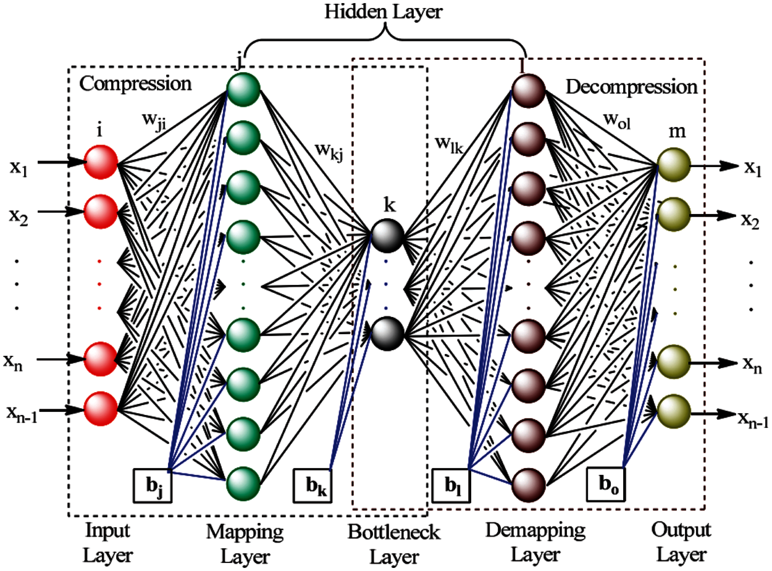
Figure 2: Architecture of deep autoencoder neural network (DANN)
The proposed DANN has the following mathematical model form:
where x donates the input vectors, ymdonates the mapping layer, t donates the bottleneck layer, yddonates the demapping layer, and
which is also called the reconstruction error.
3.3 Objective Functions for Autoencoder Neural Network Training
Apart from the reconstruction error specified in Eq. (2), three objective functions can be used to train autoencoder neural networks. We describe two alternative objective functions in this section: hierarchical error and denoising criterion. The authors in [60] proposed the concept of hierarchical error to establish a hierarchy (i.e., relative importance) amongst non-linear principal components Analysis (PCA), which is utilizing the reconstruction error as the objective function [61]. Thus, it demonstrated that maximization of the principal variable variance is equal to the residual variance minimization in linear PCA. Accordingly, the reconstruction of hierarchical error could be described as:
The authors in [62] suggested the denoising criterion to derive more stable principal components. To employ the denoising criterion, the corrupted input x is produced by adding noise to the original input x, like masking noise and Gaussian noise. Subsequently, the autoencoder neural network is trained to retrieve the original input using the corrupted data as input. Finally, the denoising criterion was used to demonstrate the ability of autoencoder neural networks to learn a lower-dimensional manifold. Thus, it will capture more essential patterns in the original data. Fig. 3 summarizes the three-goal functions schematically.
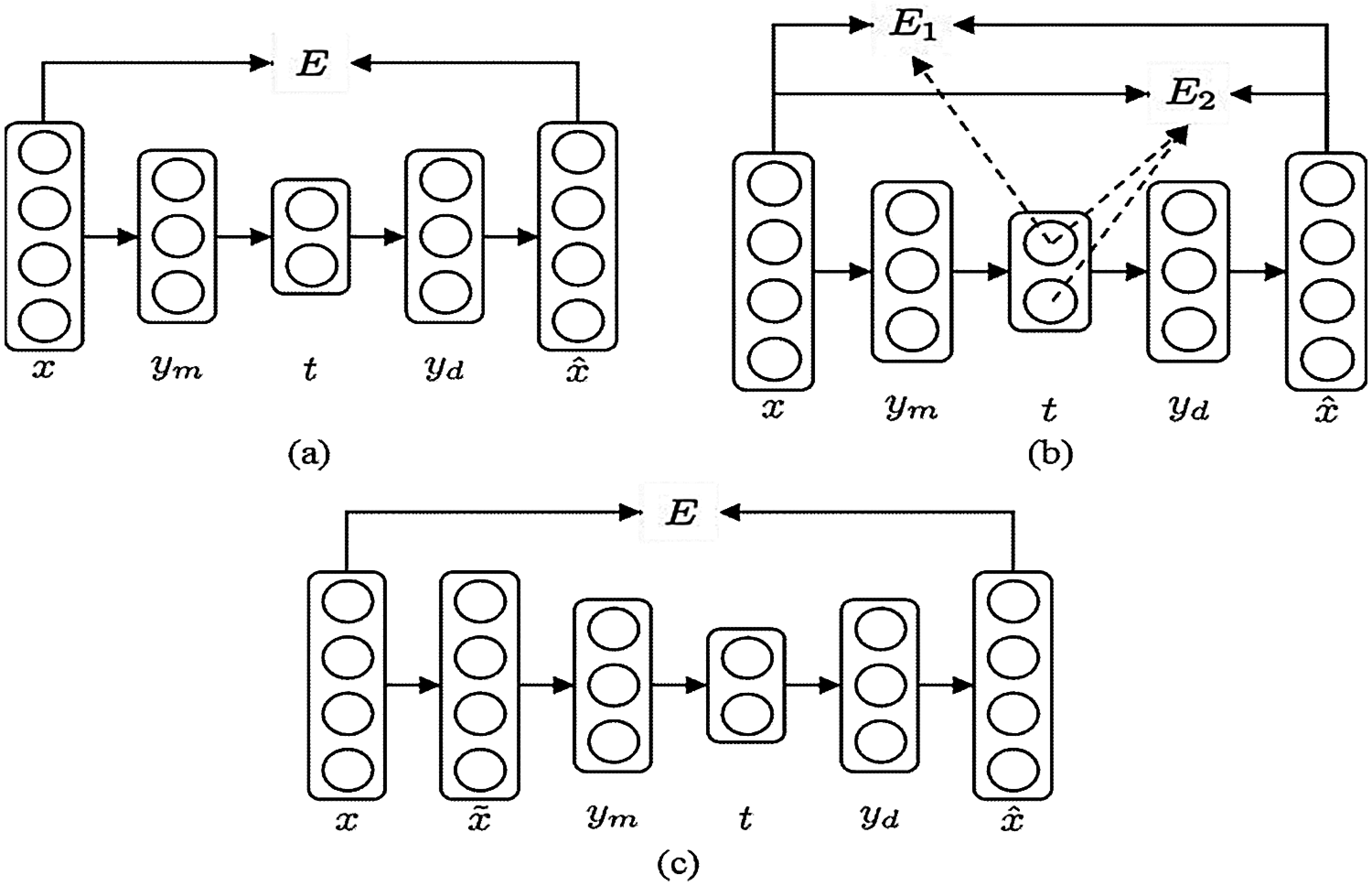
Figure 3: Different objective functions are depicted schematically: (a) Reconstruction error; (b) Hierarchical error; and (c) Denoising criterion [61]
Based on the above, we have designed a similar procedure for dimensionality reduction utilizing DANN model. First, the matrix of the original data is partitioned into two split sets, to contain only the usual operating data. One set for the training purpose and another for DANN model testing. Second, the autoencoder neural network is trained to make use of the training dataset. Once it is trained, the autoencoder neural network start computing the principal components and residuals by feeding a new data sample. This is followed by determining the T2 and Q statistics as follows:
where tk denotes the principal component value of kth in the latest sample of data, and σk denotes the kth principal component standard deviation as determined from the training dataset. It is a worth mention that the upper control limits were set with assuming the compliance of the data with a multivariate normal distribution. Thus, a different approach was followed in this work by calculating the upper control limits for two statistics directly from the given large dataset without assuming any possible distribution form. For instance, with a hundred samples of normal training data, the next biggest T2 (or Q) value is chosen as the upper control limit to attain a false alarm rate of 0.01.
3.4 Synthetic Minority Oversampling Technique (SMOTE)
Resampling the data, including undersampling and oversampling, is one of the prominent approaches to relieve ths issue of imbalanced dataset [63]. Oversampling techniques are preferable over undersampling techniques in most circumstances [64]. Synthetic Minority Oversampling Technique (SMOTE) is a well-known oversampling technique whereby synthetic samples for the minority class are produced. SMOTE techniques aids in overcoming the overfitting issue caused by random oversampling. The technique concentrates on the feature space to create new instances by interpolating among positive instances that are close together [65].
Adam [66] is a deep neural network training-specific adaptive learning rate optimization algorithm. It was firstly introduced in 2014, and it received a high attraction from a vast number of researchers due to its high performance compared to SGD or RMSprop.
The algorithm make use of adaptive learning rate techniques to determine the learning rates for each parameter individually. Adam algorithm is extremely efficient when dealing with complex problems involving a large number of variables or records. It is reliable and needs less memory. It is a combination of the ‘gradient descent with momentum and the ‘RMSP’ methods. The momentum method accelerates the gradient descent algorithm by taking the ‘exponentially weighted average’ of the gradients into account. In addition, it utilises the advantages of Adagrad [67] to perform well in environments with sparse gradients, but it struggles with non-convex optimization of neural networks. It also use the advantage of Root Mean Square Propagation (RMSprop) [68] to address some of Adagrad's shortcomings and to perform well in online settings. Utilizing averages causes this method to converge to the bare minimum more quickly.
Hence,
where, mt denotes gradients aggregate at time t (present), mt -- 1 is the aggregate of gradients at time t−1 (prior), Wt is the weights at time t, Wt+1 is the weights at time t+1, αt is the learning rate at time t, ∂L is the derivative of loss function, ∂Wt is the weights derivative at time t, β is the moving average parameter.
RMSprop is an adaptive learning method that attempts to boost AdaGrad. Rather than computing the cumulative number of squared gradients as AdaGrad does, it computes an ‘exponential moving average’.
Therefore,
where, Wt is the weights at time t, Wt+1 is the weights at time t+1, αt is the learning rate at time t, ∂L is the loss function derivative ∂Wt is the derivative of weights at time t, Vt is the sum of the square of past gradients, β is the moving average parameter ɛ is the small positive constant. Thus, the positive/strengths attributes of RMSprop and AdaGrad techniques are inherited by Adam optimizer, which builds on them to provide a more optimized gradient descent. By taking the equations utilized in the aforementioned two techniques, we get the final representation of Adam optimizer as follows:
where, β1 and β2 are the average decay rates of gradients in the aforementioned two techniques. α is the step size parameter/learning rate (0.01)
This section summarizes the experimental findings and discusses their significance for the different approaches including DANN with Adam optimizer, DANN with SGD optimizer, DANN with RMSprop optimizer, and DANN with Adamax optimizer. Tab. 1 shows the experimental results for the proposed DANN model with different optimizers methods.

4.1 Deep Autoencoder with Adam Optimizer
As depicted in Tab. 1, DANN model was tested independently without any optimization method, as shown in the column labeled “Deep autoencoder”. The achieved results are 95.91% for 10 iterations in average. To improve this result, Adam optimizer method was integrated with the proposed DANN model. As shown in the third column, the model performs better, and it was able to detect the anomaly in the dataset with an accuracy of 97.36%. Fig. 4a depicts the result of anomaly detection accuracy for autoencoder neural network with Adam optimizer and Fig. 4b sows the proposed model loss.
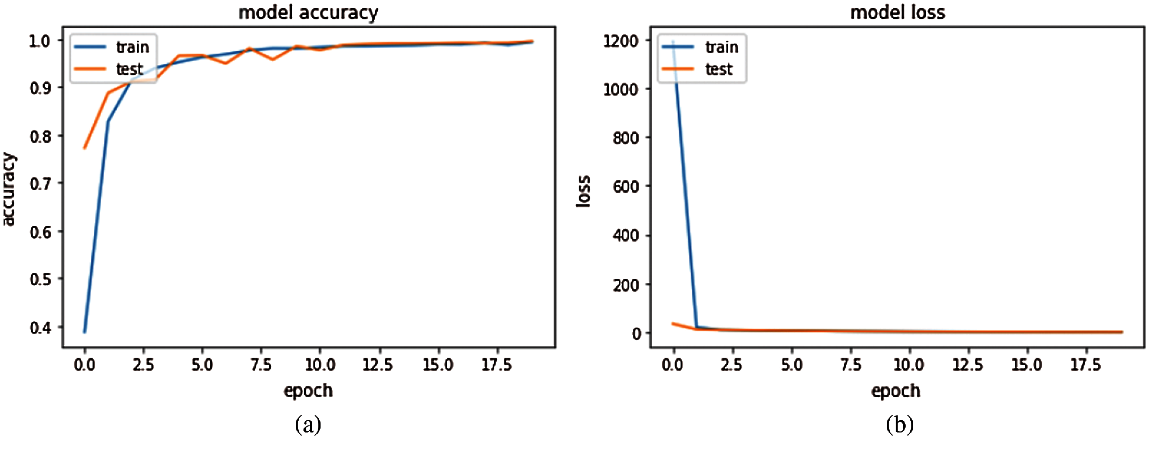
Figure 4: Accuracy and loss function results for autoencoder neural network with Adam optimizer: (a) Accuracy of the proposed hybrid model; (b) Loss function of the proposed hybrid model
4.2 Deep Autoencoder with RMSprop Optimizer
Fig. 5 shows the accuracy and loss function for the autoencoder neural network with RMSprop optimizer for both testing and training. Fig. 5a has presented the accuracy of the proposed hybrid model and Fig. 5b is presented the loss function of the proposed hybrid model with RMSprop optimizer algorithm.

Figure 5: Accuracy and loss function results for deep autoencoder neural network with RMSprop optimizer algorithm: (a) Accuracy of the proposed hybrid model; (b) Loss function of the proposed hybrid model
4.3 Deep Autoencoder with the Adamax Optimizer
The vt element in the Adam update rule scales the gradient in reverse correspondingly to the ℓ2 norm of the previous gradients (by the vt−1 term) and current gradient gt2 as presented in Eq. (9). Figs. 6a and 6b show the accuracy and loss function results for deep autoencoder neural network with the Admax optimizer method. However, this approach has superbases other proposed modes with an accuracy of 99.40% and minimal loss as shown in Fig. 6b.

Figure 6: Accuracy and loss function results for deep autoencoder neural network with the Admax optimizer method: (a) Accuracy of the proposed hybrid model; (b) Loss function of the proposed hybrid model
Fig. 5 shows the results of training and testing accuracy and loss function for the autoencoder neural network with RMSprop optimizer. Fig. 5a has presented the accuracy of the proposed hybrid model and Fig. 5b is presented the loss function of the proposed hybrid model with RMSprop optimizer algorithm.
Five measurement metrics are utilized to evaluate the performance of our experiment: Accuracy, Precision, Recall rate, F1-Score, and receiver operating characteristics (ROC). Accuracy is defined as the proportion of correctly classified samples and has the following formula:
Precision is characterized as the proportion of those who truly belong to Category-A in all samples classified as such. In general, the higher the Precision, the lower the system's False Alarm Rate (FAR).
The recall rate indicates the proportion of all samples categorized as Category-A that are ultimately classified as such. The recall rate is a measure of a system's capability to detect anomalies. The greater it is, the more anomalous traffic is correctly observed.
The F1-score enables the combination of precision and recall into a single metric that encompasses both properties.
TP, FP, TN, FN represent True Positive, False Positive, True Negative and False Negative, respectively.
Accuracy is the most widely used metric for models trained using balanced datasets. This indicates the fraction of correctly estimated samples to the overall number of samples under evaluation for the model. Fig. 7 shows the accuracy scores for the proposed anomaly detection models, determined from an independent test set. As depicted in Fig. 7, out of five proposed models, the DANN-based Adamax optimizer model achieved an accuracy score of 99.40% followed by a 90.36% score of DANN-based Adam optimizer and DANN based objective function model. Although accuracy is a popular standard measure, it has drawbacks; mainly when there is a class imbalance in samples, it is often used along with other measures like F1 score or matthew's correlation coefficient.

Figure 7: Precision, recall, F1-score and AUC achieved by DANN-based anomaly detection models
F1-score is frequently employed in circumstances where an optimum integration of precision and recall is necessary. It is the harmonic mean of precision and recall scores of a model. Thus, the F1 score can be defined as given in Eq. (13). Fig. 7 shows the F1 prediction values for anomaly detection models based on the five DANNs, which confirms the earlier performance validated using the AUC ratings. The DANN-based Adam optimizer model achieved an optimal F1 score of 0.9811, while the DANN-based Adamax optimizer model obtained second place with an F1 score of 0.9649. DANN and DANN-based SGD optimizer models showed comparable performance and achieved an F1 score of 0.9376 and 0.8823, respectively. DANN with RMSprop optimizer score was not that far from the aforementioned DANNs but earned the last place, with an F1-score of 0.8280.
A receiver operating characteristics (ROC) is a method for organizing, visualizing, and selecting classification models based on their performance [69]. Additionally, it is a valuable performance evaluation measure, ROC curves are insensitive to changes in class distribution and especially useful for problems involving skewed class distributions [69]. The ROC curve illuminates, in a sense, the cost-benefit analysis under evaluation of the classifier. The false positive (FP) ratio to total negative samples is defined as the false positive (FP) rate and measures the negative examples misclassified fraction as positive. This is considered a cost since any further action taken on the FP's result is considered a waste, as it is a positive forecast. True positive rate, defined as the fraction of correctly predicted positive samples, can be considered an advantage due to the fact correctly predicted positive samples assist the classifier in resolving the examined problem more effectively.
The proposed five models AUC values in this analysis are presented in the Legend portion of Fig. 7. It is shown clearly from Fig. 7 that the DANN-based Adamax optimizer model outperforms the rest of the methods in detection anomaly in a high dimensional real-life dataset, with an AUC value of 0.981. The model-based adam optimizer obtained the second-best prediction with an AUC value of 0.951. The AUC results obtained validate the earlier evaluation results indicated by the F1 score matric.
When optimizing classification models, cross-entropy is often utilized as a loss function. Cross-entropy as a loss function is extremely useful in binary classification problems that include the prediction of a class mark from one or more input variables. Our model attempts to estimate the target probability distribution Q as closely as possible. Thus, we can estimate the cross-entropy for an anomaly prediction in high dimensional data using the cross-entropy calculation given as follows:
• Predicted P(class0) = 1 – yhat
• Predicted P(class1) = yhat
This implies that the model explicitly predicts the probability of class 1, while the probability of class 0 is given as one minus the expected probability. Fig. 8 shows the average cross-entropy across all training data for the DANN-based adamax optimizer method, where the model has minimal function loss. Hence, this confirms that the proposed model is efficient and effective in predicting anomaly in high dimensional data.

Figure 8: DANN+Adamax optimizer model for anomaly detection using cross-entropy as a loss function
To detect the anomaly in high dimensionality industrial gas turbine dataset, we were unable to find any research contribution that has been evaluated, but we have compared the results with the two recently proposed approaches for anomaly detection in the high dimensional dataset [70,71] shown in Tab. 2. The comparison is only shown for metrics available, but essentially, it shows the reader the promising results of the proposed DANN-based Adamax optimizer during the training process of the proposed model. The results show that the proposed method surpasses the two previous methods for detection anomaly in the high dimensional data set.
As presented in Tab. 2, the proposed detection model obtained a better result in detecting the anomaly and overcoming dimensionality's curse without needing any complex and labor-intensive feature extraction. This is possible due to the inherent capability of DANNs to learn the task-specific feature presentations automatically. Thus, the proposed DANN outperform the anomaly detection approach that is based on an Autoregressive Flow-based (ADAF) model [70] and the hybrid semi-supervised anomaly detection model suggested by [71].

This study proposed an efficient and improved deep autoencoder based anomaly detection approach in real industrial gas turbine data set. The proposed approach aims at improving the accuracy of anomaly detection by reducing the dimensionality in the large gas turbine data. The proposed deep autoencoder neural networks (DANN) were integrated and tested with several well-known optimization methods for the deep autoencoder training process. The proposed DANN approach was able to overcome the curse of dimensionality effectively. It evaluated based on commonly used evaluation measures to evaluate and validate the DANN models performance. The DANN-based Adamax optimization method has achieved the best performance with an accuracy of 99.40%, F1-score of 0.9649 and an AUC rate of 0.9649. At the same time, the DANN-based SGD optimization method obtained the worse performance in anomaly detection in the high dimensional dataset.
Funding Statement: This research/paper was fully supported by Universiti Teknologi PETRONAS, under the Yayasan Universiti Teknologi PETRONAS (YUTP) Fundamental Research Grant Scheme (YUTP-015LC0-123).
Conflicts of Interest: The authors declare that they have no conflicts of interest to report regarding the present study.
1. F. Cappa, R. Oriani, E. Peruffo and I. McCarthy, “Big data for creating and capturing value in the digitalized environment: Unpacking the effects of volume, variety, and veracity on firm performance,” Journal of Product Innovation Management, vol. 38, no. 1, pp. 49–67, 2021. [Google Scholar]
2. F. Pigni, G. Piccoli and R. Watson, “Digital data streams: Creating value from the real-time flow of big data,” California Management Review, vol. 58, no. 3, pp. 5–25, 2016. [Google Scholar]
3. A. Sestino, M. I. Prete, L. Piper and G. Guido, “Internet of things and big data as enablers for business digitalization strategies,” Technovation, vol. 98, no. 1, pp. 102173, 2020. [Google Scholar]
4. A. Gandomi and M. Haider, “Beyond the hype: Big data concepts, methods, and analytics,” International Journal of Information Management, vol. 35, no. 2, pp. 137–144, 2015. [Google Scholar]
5. S. Thudumu, P. Branch, J. Jin and J. J. Singh, “A comprehensive survey of anomaly detection techniques for high dimensional big data,” Journal of Big Data, vol. 7, no. 1, pp. 1–30, 2020. [Google Scholar]
6. I. Lee, “Big data: Dimensions, evolution, impacts, and challenges,” Business Horizons, vol. 60, no. 3, pp. 293–303, 2017. [Google Scholar]
7. A. Oussous, F.-Z. Benjelloun, A. A. Lahcen and S. Belfkih, “Big data technologies: A survey,” Journal of King Saud University-Computer and Information Sciences, vol. 30, no. 4, pp. 431–448, 2018. [Google Scholar]
8. A. V. Sadr, B. A. Bassett and M. Kunz, “A flexible framework for anomaly detection via dimensionality reduction,” Neural Computing and Applications, vol. 10, no. 1, pp. 1–11, 2021. [Google Scholar]
9. V. Chandola, A. Banerjee and V. Kumar, “Anomaly detection: A survey,” ACM Computing Surveys (CSUR), vol. 41, no. 3, pp. 1–58, 2009. [Google Scholar]
10. A. Patcha and J.-M. Park, “An overview of anomaly detection techniques: Existing solutions and latest technological trends,” Computer Networks, vol. 51, no. 12, pp. 3448–3470, 2007. [Google Scholar]
11. A. O. Balogun, S. Basri, S. J. Abdulkadir, V. E. Adeyemo, A. A. Imam et al., “Software defect prediction: Analysis of class imbalance and performance stability,” Journal of Engineering Science and Technology, vol. 14, no. 6, pp. 3294–3308, 2019. [Google Scholar]
12. D. Becker, T. D. King and B. McMullen, “Big data, big data quality problem,” in 2015 IEEE Int. Conf. on Big Data (Big DataSanta Clara, CA, USA, pp. 2644–2653, 2015. [Google Scholar]
13. M. Novotny and H. Hauser, “Outlier-preserving focus+context visualization in parallel coordinates,” IEEE Transactions on Visualization and Computer Graphics, vol. 12, no. 5, pp. 893–900, 2006. [Google Scholar]
14. Y. Zhai, Y.-S. Ong and I. W. Tsang, “The emerging big dimensionality,” IEEE Computational Intelligence Magazine, vol. 9, no. 3, pp. 14–26, 2014. [Google Scholar]
15. L. Selicato, F. Esposito, G. Gargano, M. C. Vegliante, G. Opinto et al., “A new ensemble method for detecting anomalies in gene expression matrices,” Mathematics, vol. 9, no. 8, pp. 882, 2021. [Google Scholar]
16. H. Zenati, M. Romain, C.-S. Foo, B. Lecouat and V. Chandrasekhar, “Adversarially learned anomaly detection,” in 2018 IEEE Int. Conf. on Data Mining (ICDMSingapore, pp. 727–736, 2018. [Google Scholar]
17. X. Zhou, Y. Hu, W. Liang, J. Ma and Q. Jin, “Variational LSTM enhanced anomaly detection for industrial big data,” IEEE Transactions on Industrial Informatics, vol. 17, no. 5, pp. 3469–3477, 2020. [Google Scholar]
18. A. O. Balogun and R. G. Jimoh, “Anomaly intrusion detection using an hybrid of decision tree and K-nearest neighbor,” Journal of Advances in Scientific Research & Applications (JASRA), vol. 2, no. 1, pp. 67–74, 2015. [Google Scholar]
19. F. Angiulli and C. Pizzuti, “Fast outlier detection in high dimensional spaces,” in European Conf. on Principles of Data Mining and Knowledge Discovery, Springer, Berlin, Heidelberg, pp. 15–27, 2002. [Google Scholar]
20. V. Hautamaki, I. Karkkainen and P. Franti, “Outlier detection using k-nearest neighbour graph,” in Proc. of the 17th Int. Conf. on Pattern Recognition, 2004, ICPR 2004, Cambridge, UK, vol. 3, pp. 430–433, 2004. [Google Scholar]
21. S. Ramaswamy, R. Rastogi and K. Shim, “Efficient algorithms for mining outliers from large data sets,” in Proc. of the 2000 ACM SIGMOD Int. Conf. on Management of Data, Dallas, Texas, USA, pp. 427–438, 2000. [Google Scholar]
22. A. Zimek, R. J. Campello and J. Sander, “Ensembles for unsupervised outlier detection: Challenges and research questions a position paper,” Acm Sigkdd Explorations Newsletter, vol. 15, no. 1, pp. 11–22, 2014. [Google Scholar]
23. J. R. Pasillas-Díaz and S. Ratté, “Bagged subspaces for unsupervised outlier detection,” Computational Intelligence, vol. 33, no. 3, pp. 507–523, 2017. [Google Scholar]
24. L. Wilkinson, “Visualizing big data outliers through distributed aggregation,” IEEE Transactions on Visualization and Computer Graphics, vol. 24, no. 1, pp. 256–266, 2017. [Google Scholar]
25. P. D. Talagala, R. J. Hyndman and K. Smith-Miles, “Anomaly detection in high-dimensional data,” Journal of Computational and Graphical Statistics, vol. 30, pp. 1–15, 2020. [Google Scholar]
26. R. Chalapathy, A. K. Menon and S. Chawla, “Anomaly detection using one-class neural networks,” ArXiv Preprint ArXiv: 1802.06360, 2018. [Google Scholar]
27. P. Wu, J. Liu and F. Shen, “A deep one-class neural network for anomalous event detection in complex scenes,” IEEE Transactions on Neural Networks and Learning Systems, vol. 31, no. 7, pp. 2609–2622, 2019. [Google Scholar]
28. E. Favarelli, E. Testi and A. Giorgetti, “One class classifier neural network for anomaly detection in low dimensional feature spaces,” in 2019 13th Int. Conf. on Signal Processing and Communication Systems (ICSPCSGold Coast, QLD, Australia, pp. 1–7, 2019. [Google Scholar]
29. P. Malhotra, A. Ramakrishnan, G. Anand, L. Vig, P. Agarwal et al., “LSTM-Based encoder-decoder for multi-sensor anomaly detection,” ArXiv Preprint ArXiv: 1607.00148, 2016. [Google Scholar]
30. H. Nguyen, K. P. Tran, S. Thomassey and M. Hamad, “Forecasting and anomaly detection approaches using LSTM and LSTM autoencoder techniques with the applications in supply chain management,” International Journal of Information Management, vol. 57, no. 1, pp. 102282, 2021. [Google Scholar]
31. M. Said Elsayed, N.-A. Le-Khac, S. Dev and A. D. Jurcut, “Network anomaly detection using lstm based autoencoder,” in Proc. of the 16th ACM Symposium on QoS and Security for Wireless and Mobile Networks, New York, US, pp. 37–45, 2020. [Google Scholar]
32. R. Chalapathy and S. Chawla, “Deep learning for anomaly detection: A survey,” ArXiv Preprint ArXiv: 1901.03407, 2019. https://scholar.google.com/scholar?hl=en&as_sdt=0%2C5&q=Deep+learning+for+anomaly+detection%3A+A+survey&btnG=#d=gs_cit&u=%2Fscholar%3Fq%3Dinfo%3AJrT0WQ7JDc8J%3Ascholar.google.com%2F%26output%3Dcite%26scirp%3D0%26hl%3Den. [Google Scholar]
33. R. A. A. Habeeb, F. Nasaruddin, A. Gani, I. A. T. Hashem, E. Ahmed et al., “Real-time big data processing for anomaly detection: A survey,” International Journal of Information Management, vol. 45, no.1, pp. 289–307, 2019. [Google Scholar]
34. F. Di Mattia, P. Galeone, M. De Simoni and E. Ghelfi, “A survey on gans for anomaly detection,” ArXiv Preprint ArXiv: 1906.11632, 2019. https://scholar.google.com/scholar?cluster=13075903367544403689&hl=en&as_sdt=0,5#d=gs_cit&u=%2Fscholar%3Fq%3Dinfo%3A6XbRa9XwdrUJ%3Ascholar.google.com%2F%26output%3Dcite%26scirp%3D0%26scfhb%3D1%26hl%3Den. [Google Scholar]
35. G. Pang, L. Cao and C. Aggarwal, “Deep learning for anomaly detection: challenges, methods, and opportunities,” in Proc. of the 14th ACM Int. Conf. on Web Search and Data Mining, Jerusalem, Israel, pp. 1127–1130, 2021. [Google Scholar]
36. M. M. Breunig, H.-P. Kriegel, R. T. Ng and J. Sander, “LOF: identifying density-based local outliers,” in Proc. of the 2000 ACM SIGMOD Int. Conf. on Management of Data, Dallas, Texas USA, pp. 93–104, 2000. [Google Scholar]
37. H.-P. Kriegel, P. Kröger, E. Schubert and A. Zimek, “Outlier detection in axis-parallel subspaces of high dimensional data,” in Pacific-Asia Conf. on Knowledge Discovery and Data Mining, Berlin, Heidelberg, Springer, pp. 831–838, 2009. [Google Scholar]
38. J. Zhang, X. Yu, Y. Li, S. Zhang, Y. Xun et al., “A relevant subspace based contextual outlier mining algorithm,” Knowledge-Based Systems, vol. 99, no. 1, pp. 1–9, 2016. [Google Scholar]
39. J. K. Dutta, B. Banerjee and C. K. Reddy, “RODS: Rarity based outlier detection in a sparse coding framework,” IEEE Transactions on Knowledge and Data Engineering, vol. 28, no. 2, pp. 483–495, 2015. [Google Scholar]
40. B. Van Stein, M. Van Leeuwen and T. Bäck, “Local subspace-based outlier detection using global neighbourhoods,” in 2016 IEEE Int. Conf. on Big Data (Big DataWashington, DC, USA, pp. 1136–1142, 2016. [Google Scholar]
41. C. C. Aggarwal and S. Y. Philip, “An effective and efficient algorithm for high-dimensional outlier detection,” The VLDB Journal, vol. 14, no. 2, pp. 211–221, 2005. [Google Scholar]
42. C. C. Aggarwal and S. Sathe, “Theoretical foundations and algorithms for outlier ensembles,” Acm Sigkdd Explorations Newsletter, vol. 17, no. 1, pp. 24–47, 2015. [Google Scholar]
43. A. Theissler, “Detecting known and unknown faults in automotive systems using ensemble-based anomaly detection,” Knowledge-Based Systems, vol. 123, no. 1, pp. 163–173, 2017. [Google Scholar]
44. A. Lazarevic and V. Kumar, “Feature bagging for outlier detection,” in Proc. of the Eleventh ACM SIGKDD Int. Conf. on Knowledge Discovery in Data Mining, Chicago, Illinois, USA, pp. 157–166, 2005. [Google Scholar]
45. H. V. Nguyen, H. H. Ang and V. Gopalkrishnan, “Mining outliers with ensemble of heterogeneous detectors on random subspaces,” in Int. Conf. on Database Systems for Advanced Applications, Tsukuba, Japan, Springer, pp. 368–383, 2010. [Google Scholar]
46. F. Keller, E. Muller and K. Bohm, “HiCS: High contrast subspaces for density-based outlier ranking,” in 2012 IEEE 28th Int. Conf. on Data Engineering, Denver, CO, USA, IEEE, pp. 1037–1048, 2012. [Google Scholar]
47. J. L. Fernández-Martínez and Z. Fernández-Muñiz, “The curse of dimensionality in inverse problems,” Journal of Computational and Applied Mathematics, vol. 369, no. 1, pp. 112571, 2020. [Google Scholar]
48. M. A. Bessa, R. Bostanabad, Z. Liu, A. Hu, D. W. Apley et al., “A framework for data-driven analysis of materials under uncertainty: Countering the curse of dimensionality,” Computer Methods in Applied Mechanics and Engineering, vol. 320, no. 1, pp. 633–667, 2017. [Google Scholar]
49. A. Subasi, “Machine learning techniques,” in Practical Machine Learning for Data Analysis Using Python, Jeddah, Saudi Arabia, Academic Press, pp. 1–520, 2020. [Google Scholar]
50. J. Hajewski, S. Oliveira and X. Xing, “Distributed evolution of deep autoencoders,” ArXiv Preprint ArXiv: 2004.07607, 2020. https://scholar.google.com/scholar?hl=en&as_sdt=0%2C5&q=Distributed+evolution+of+deep+autoencoders&btnG=#d=gs_cit&u=%2Fscholar%3Fq%3Dinfo%3AN8U4HJ5V4GMJ%3Ascholar.google.com%2F%26output%3Dcite%26scirp%3D0%26hl%3Den. [Google Scholar]
51. N. Renström, P. Bangalore and E. Highcock, “System-wide anomaly detection in wind turbines using deep autoencoders,” Renewable Energy, vol. 157, no.1, pp. 647–659, 2020. [Google Scholar]
52. J. Abeßer, S. I. Mimilakis, R. Gräfe, H. Lukashevich and I. D. M. T. Fraunhofer “Acoustic scene classification by combining autoencoder-based dimensionality reduction and convolutional neural networks,” in Proc. of the Detection and Classification of Acoustic Scenes and Events 2017 Workshop (DCASE2017), Munich, Germany, pp. 7--11, 2017. [Google Scholar]
53. S. Alsenan, I. Al-Turaiki and A. Hafez, “Autoencoder-based dimensionality reduction for QSAR modeling,” in 2020 3rd Int. Conf. on Computer Applications Information Security (ICCAIS), Riyadh, Saudi Arabia, pp. 1–4, 2020. [Google Scholar]
54. V. Q. Nguyen, V. H. Nguyen and N. A. Le-Khac, “Clustering-based deep autoencoders for network anomaly detection,” in Int. Conf. on Future Data and Security Engineering, Springer, Cham, pp. 290–303, 2020. [Google Scholar]
55. M. Ramamurthy, Y. H. Robinson, S. Vimal and A. Suresh, “Auto encoder-based dimensionality reduction and classification using convolutional neural networks for hyperspectral images,” Microprocessors and Microsystems, vol. 79, no. 1, pp. 103280, 2020. [Google Scholar]
56. G. M. San, E. López Droguett, V. Meruane and M. D. Moura, “Deep variational auto-encoders: A promising tool for dimensionality reduction and ball bearing elements fault diagnosis,” Structural Health Monitoring, vol. 18, no. 4, pp. 1092–1128, 2019. [Google Scholar]
57. Z. Chen, C. K. Yeo, B. S. Leeand C. T. Lau, “Autoencoder-based network anomaly detection,” in 2018 Wireless Telecommunications Symposium (WTS), Phoenix, AZ, USA, pp. 1–5, 2018. [Google Scholar]
58. S. Russo, A. Disch, F. Blumensaat and K. Villez, “Anomaly detection using deep autoencoders for in-situ wastewater systems monitoring data,” ArXiv Preprint, ArXiv: 2002.03843, 2020. [Google Scholar]
59. M. A. Albahar and M. Binsawad, “Deep autoencoders and feedforward networks based on a new regularization for anomaly detection,” Security and Communication Networks, vol. 2020, pp. 7086367, 2020. https://doi.org/10.1155/2020/7086367. [Google Scholar]
60. M. Scholz and R. Vigário, “Nonlinear PCA: A new hierarchical approach,” in Esann, Bruges, Belgium, pp. 439–444, 2002. [Google Scholar]
61. S. Heo and J. H. Lee, “Statistical process monitoring of the Tennessee eastman process using parallel auto associative neural networks and a large dataset,” Processes, vol. 7, no. 7, pp. 4 11, 2019. [Google Scholar]
62. P. Vincent, H. Larochelle, I. Lajoie, Y. Bengio and P. A. Manzagol, “Stacked denoising autoencoders: Learning useful representations in a deep network with a local denoising criterion,” Journal of Machine Learning Research, vol. 11, no. 1, pp. 3371–3408, 2010. [Google Scholar]
63. A. Fernández, S. Garcia, F. Herrera and N. V. Chawla, “SMOTE for learning from imbalanced data: Progress and challenges, marking the 15-year anniversary,” Journal of Artificial Intelligence Research, vol. 61, no. 1, pp. 863–905, 2018. [Google Scholar]
64. P. Skryjomski and B. Krawczyk, “Influence of minority class instance types on SMOTE imbalanced data oversampling,” in First International Workshop on Learning with Imbalanced Domains: Theory and Applications, Richmond, VA, USA, pp. 7–21, 2017. [Google Scholar]
65. L. Lusa, “Class prediction for high-dimensional class-imbalanced data,” BMC Bioinformatics, vol. 11, no. 1, pp. 1–17, 2010. [Google Scholar]
66. D. P. Kingma and J. Ba, “Adam: A method for stochastic optimization,” ArXiv Preprint ArXiv: 1412.6980, 2014. [Google Scholar]
67. J. Duchi, E. Hazan and Y. Singer, “Adaptive sub gradient methods for online learning and stochastic optimization,” Journal of Machine Learning Research, vol. 12, no. 7, pp. 2121–2159, 2011. [Google Scholar]
68. V. Durairajah, S. Gobee and A. Muneer, “Automatic vision based classification system using DNN and SVM classifiers,” in 2018 3rd Int. Conf. on Control, Robotics and Cybernetics (CRCPenang, Malaysia, pp. 6–14, 2018. [Google Scholar]
69. Y. Yu, P. Lv X. Tong, and J. Dong, “Anomaly detection in high-dimensional data based on autoregressive flow,” in Int. Conf. on Database Systems for Advanced Applications, Springer, Cham, pp. 125–140, 2020. [Google Scholar]
70. H. Song, Z. Jiang, A. Men and B. Yang, “A hybrid semi-supervised anomaly detection model for high-dimensional data,” Computational Intelligence and Neuroscience, vol. 17, no. 1, pp. 1–9, 2017. [Google Scholar]
71. T. Fawcett, “An introduction to ROC analysis,” Pattern Recognition Letters, vol. 27, no. 8, pp. 861–874, 2006. [Google Scholar]
 | This work is licensed under a Creative Commons Attribution 4.0 International License, which permits unrestricted use, distribution, and reproduction in any medium, provided the original work is properly cited. |