Computers, Materials & Continua DOI:10.32604/cmc.2022.020689
Article

Accurate Multi-Site Daily-Ahead Multi-Step PM2.5 Concentrations Forecasting Using Space-Shared CNN-LSTM

Xiaorui Shao and Chang Soo Kim*

Department of Information Systems, Pukyong National University, Busan, 608737, Korea
*Corresponding Author: Chang Soo Kim. Email: cskim@pknu.ac.kr
Received: 03 June 2021; Accepted: 05 August 2021

Abstract: Accurate multi-step PM2.5 (particulate matter with diameters ≤2.5um) concentration prediction is critical for humankinds’ health and air population management because it could provide strong evidence for decision-making. However, it is very challenging due to its randomness and variability. This paper proposed a novel method based on convolutional neural network (CNN) and long-short-term memory (LSTM) with a space-shared mechanism, named space-shared CNN-LSTM (SCNN-LSTM) for multi-site daily-ahead multi-step PM2.5 forecasting with self-historical series. The proposed SCNN-LSTM contains multi-channel inputs, each channel corresponding to one-site historical PM2.5 concentration series. In which, CNN and LSTM are used to extract each site's rich hidden feature representations in a stack mode. Especially, CNN is to extract the hidden short-time gap PM2.5 concentration patterns; LSTM is to mine the hidden features with long-time dependency. Each channel extracted features are merged as the comprehensive features for future multi-step PM2.5 concentration forecasting. Besides, the space-shared mechanism is implemented by multi-loss functions to achieve space information sharing. Therefore, the final features are the fusion of short-time gap, long-time dependency, and space information, which enables forecasting more accurately. To validate the proposed method's effectiveness, the authors designed, trained, and compared it with various leading methods in terms of RMSE, MAE, MAPE, and R2 on four real-word PM2.5 data sets in Seoul, South Korea. The massive experiments proved that the proposed method could accurately forecast multi-site multi-step PM2.5 concentration only using self-historical PM2.5 concentration time series and running once. Specifically, the proposed method obtained averaged RMSE of 8.05, MAE of 5.04, MAPE of 23.96%, and R2 of 0.7 for four-site daily ahead 10-hour PM2.5 concentration forecasting.

Keywords: PM2.5 forecasting; CNN-LSTM; air quality management;; multi-site multi-step forecasting

1  Introduction

With the rapid development of industrialization and economics, air pollution is becoming a serious environmental issue, which threatens humankinds’ health significantly. The PM2.5 concentration could reflect the air quality and has been widely applied for air quality management and control [1,2]. Thus, accurate PM2.5 forecasting has been a hot topic and attracted massive attention as it could provide in-time and robust evidence to help decision-makers make appropriate policies to manage and improve air quality. There are two kinds of PM2.5 forecasting tasks: one-step (also called single step) and multi-step. One-step PM2.5 forecasting provides one-step ahead information, while multi-step forecasting provides multi-step ahead information. Citizens could benefit from them by taking peculiar actions in advance.

The current methods for PM2.5 forecasting could be divided into regression-based, time series-based, and learning-based methods (also called data-driven methods) [3]. Regression-based methods aim to find the linear patterns among multi-variables to build the regression expression. e.g., Zhao et al. [4] applied multi-linear regression (MLR) with meteorological factors including wind velocity, temperature, humidity, and other gaseous pollutants (SO2, NO2, CO, and O3) for one-step PM2.5 forecasting. Ul-saufie et al. [5] applied principal component analysis (PCA) to select the most correlated variables to forecast one-step PM10 with MLR model. Time series-based methods aim at mining the PM2.5 series’ hidden patterns between past historical and future values. The most popular time series-based method is auto-regressive integrated move average (ARIMA), which models the relationship between historical and future values by calculating three parameters: (p,d,q). It has been widely used for one-step PM2.5 and air quality index (AQI) forecasting [6,7]. However, both regression-based and time-series methods only consider the linear correlations in those meteorological factors while it is usually nonlinear [8]. Thereby, the forecasting accuracy is still not satisfactory.

Learning-based methods, including shallow learning and deep learning, could extract the nonlinear relationships between meteorological variables and future PM2.5 concentrations that have been applied for PM2.5 forecasting. Support vector machine (SVM), one of the most attractive shallow learning-based methods, uses various nonlinear kernels to map the original meteorological factors into a higher-dimension panel to improve forecasting accuracy. e.g., Deters et al. [9] applied SVM for daily PM2.5 analysis and one-step forecasting with meteorological parameters. Sun et al. [2] applied PCA to select the most correlated variables as the input of SVM for one-step PM2.5 concentration forecasting in China. ANN, another shallow learning-based method, utilizes two or three hidden layers to extract hidden patterns for PM2.5 concentration forecasting [10,11]. However, SVM requires massive memory to search the high-dimension panel and is easy to fall into overfitting [12,13]. ANN cannot extract the full hidden patterns due to it is not “deep” enough. Therefore, the forecasting accuracy is still not satisfactory and can be improved. In addition, some methods combined serval models to achieve better performance for AQI forecasting. e.g., Ausati et al. [1] combined ensemble empirical mode decomposition and general neural network (EEMD-GRNN), adaptive neuro-fuzzy inference system (ANFIS), principal component regression (PCR), and LR models for one-step PM2.5 concentration forecasting using meteorological data and corresponding air factors. Cheng et al. [7] combined ARIMA, SVM, and ANN in a linear model to predict daily PM2.5 concentrations in five of China's cities. However, those combined methods still cannot address each model's shortcoming, and they require handcrafted feature selection operations, which is time-consumption and increases the development's cost.

Deep learning technologies, including deep brief network (DBN), convolutional neural network (CNN) [14], and recurrent neural network (RNN) [15], provide a new view for PM2.5 forecasting due to their excellent feature extraction capacity. Xie et al. [16] applied a manifold learning-locally linear embedding method to reconstruct low-dimensional meteorological factors as the DBN's input for daily single-step PM2.5 forecasting in Chongqing, China. Kow et al. [17] utilized CNN and backpropagation (CNN-BP) to extract the hidden features of multi-sites in Korea with multivariate factors, including temperature, humidity, CO, and PM10, for multi-step and multi-sites hourly PM2.5 forecasting. Park et al. [18] applied CNN with nearby locations’ meteorological data for daily single-step PM2.5 forecasting. Ayturan et al. [19] utilized a combination of gated recurrent unit (GRU) and RNN to forecast hourly ahead single-step PM2.5 concentrations with meteorological and air pollution parameters. Zhang et al. [20] used VMD to obtain frequency-domain features from the historical PM2.5 series as the input of the bidirectional LSTM (Bi-LSTM) for hourly single-step PM2.5 forecasting. Moreover, some hybrid models combined CNN and LSTM have been developed for PM2.5 concentration forecasting. For instance, Qin et al. [21] used one classical CNN-LSTM to make hourly PM2.5 predictions. They collected wind speed, wind direction, temperature, historical PM2.5 series, and pollutant concentration parameters as CNN's input. CNN extracted features are fed into LSTM to mine the features consider the time dependence of pollutants for PM2.5 forecasting. Qi et al. [22] developed a novel graph convolutional network and long short-term memory networks (GC-LSTM) for single-step hourly PM2.5 forecasting. Pak et al. [23] utilized mutual information (MI) to select the most correlated factors to generate a spatiotemporal feature vector as CNN-LSTM's input to forecast daily single-step PM2.5 concentration of Beijing, China. Tab. 1 gives a summary of recent important references using deep learning for PM2.5 forecasting.

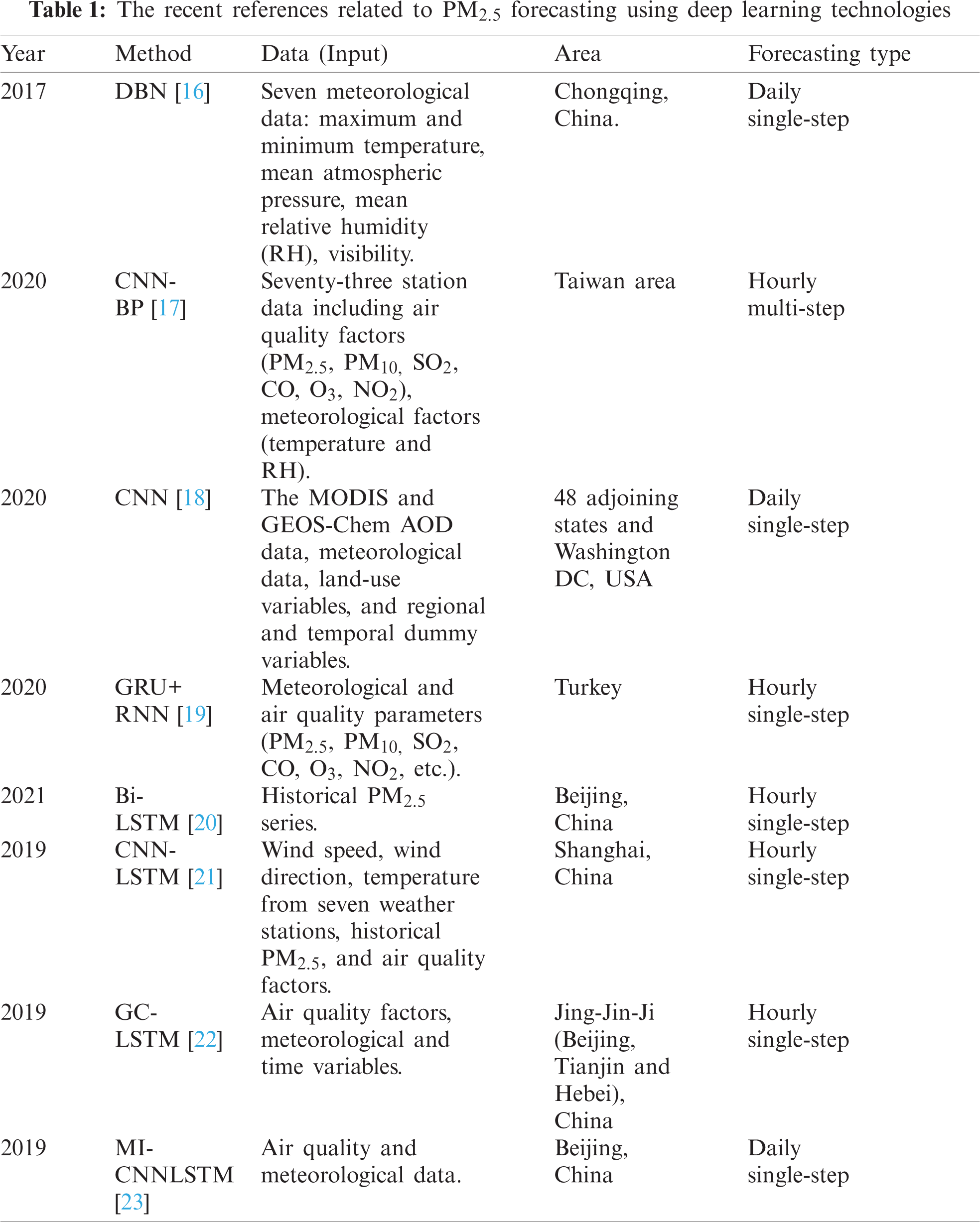
Although the above deep learning-based methods achieved good performance, Tab. 1 showed that most of them require collecting meteorological and air quality data except for [20]. Collecting those kinds of data is time-consumption and even is not available for most cases [24,25]. Besides, Zhang et al. [20] proposed method requires the PM2.5 series is long enough to do VMD decomposition while day-ahead forecasting cannot satisfy. Another observation showed that only CNN-BP [17] focused on multi-step hourly PM2.5 concentration forecasting while others are single-step, which cannot satisfy human beings’ needs. Motivated by those, this manuscript proposed a novel deep model to extract PM2.5 concentration's full hidden patterns for multi-site daily-ahead multi-step PM2.5 concentration forecasting only using self-historical series. In the proposed method, multi-channels corresponding to multi-site PM2.5 concentration series is fed into CNN-LSTM to extract rich hidden features individually. Especially, CNN is to extract short-time gap features; LSTM is to mine the features with long-time dependency from CNN extracted feature representations. Moreover, the space-shared mechanism is developed to enable space information sharing during the training process. Consequently, it could extract rich and robust features to enhance forecasting accuracy. The main contributions of this manuscript are summarized as follows:

•   To our best of understanding, we are the first to make multi-site multi-step PM2.5 forecasting with the space-sharing mechanism only using the self-historical PM2.5 series.

•   A novel framework named SCNN-LSTM with a multi-output strategy is proposed to forecast daily-ahead multi-site and multi-step PM2.5 concentrations only using self-historical PM2.5 series and running once. Sufficient comparative analysis has confirmed its effectiveness and robustness in multiple evaluation metrics, including RMSE, MAE, MAPE, and R2.

•   The effectiveness of each part in the proposed method has been analyzed.

The rest of the paper is arranged as follows. Section 2 gives a detailed description of the proposed SCNN-LSTM. The experimental verification is carried out in Section 3. Section 4 discusses the effectiveness of the proposed SCNN-LSTM for daily-ahead multi-step PM2.5 concentrations forecasting. The conclusion is conducted in Section 5.

2  The Proposed SCNN-LSTM for Multi-Step PM2.5 Forecasting

2.1 Multi-Step PM2.5 Forecasting

Assume that we collected a long PM2.5 concentration series, denoted as Eq. (1). Where the PM2.5 series consists of N values, Tt is the PM2.5 concentration value at time t.

T=[T1,T2,T3,…,Tt,…,TN],1≤t≤N(1)

The current methods for multi-step forecasting consist of direct and recursive strategies [26]. The direct strategy uses h different models fh for each step forecasting, and each step forecasting results are independent, as described in Eq. (2). The future h-step PM2.5 concentrations from time t+1 to t+hare obtained using different h models such as ARIMA, MLR, ANN, CNN, etc., with historical PM2.5 concentrations from (t−m)th to tth. However, it did not consider the influence of each step, which leads to low-precision forecasting. The recursive strategy trains one model f at h times for h-step forecasting with dynamic inputs to overcome this shortcoming. The previous-step forecasting result Tt+1 is used as the next step's input to forecast Tt+2, as described in Eq. (3). However, the accumulated error of each-step forecasting will decrease the forecasting accuracy significantly. Moreover, training one model many times is costly.

T{t+1,t+2,…,t+h}=fh(Tt−m,Tt−m+1,…,Tt−1,Tt)(2)

{Tt+1=f(Tt−m,Tt−m+1,…,Tt−1,Tt)Tt+2=f(Tt−m+1,…,Tt−1,Tt,Tt+1)Tt+3=f(Tt−m+2,…,Tt,Tt+1,Tt+2)⋮Tt+h=f(Tt+h−1−m,Tt+h−m,…,Tt+h−2,Tt+h−1)(3)

To avoid the above shortcomings, the proposed SCNN-LSTM method adopted a multi-output strategy for multi-step PM2.5 forecasting, as shown in Eq. (4). The h-step future PM2.5 concentrations T{t+1,t+2,…,t+h} are calculating by trained model f once with historical PM2.5 concentrations (Tt−n,Tt−n−1,…,Tt−1,Tt). Our purpose is to build model f to extract the full hidden feature representations that existed in the PM2.5 series to forecast accurately.

T{t+1,t+2,…,t+h}=f(Tt−m,Tt−m+1,…,Tt−1,Tt)(4)

2.2 Proposed SCNN-LSTM

The proposed SCNN-LSTM for multi-site daily-ahead multi-step PM2.5 concentration forecasting consists of four steps: input construction, feature extraction, multi-space feature sharing, output and update the network, as shown in Fig. 1. More details of each part are introduced in the following sections.

2.2.1 Input Construction

The proposed method adopted near s sites’ self-historical PM2.5 concentration series as input to mine its hidden patterns considering the influence on space. Before modeling, we utilized a non-overlapped algorithm [8] to generate each site's corresponding input matrix Sitei and h-step label matrix LabelSitei since CNN-LSTM is a supervised algorithm, as shown in Eqs. (5) and (6). Where a long time-series defined in Eq. (1) with the length of N could obtain M samples using a non-overlapped algorithm in a sample rate of m and stride k, each sample Sitei,j=[Tt−m+1,Tt−m+2,…,Tt] contains m PM2.5 values from time step (t−m+1)thtotth. Moreover, m, k, M, N, h should satisfy the constraint of Eq. (7). The ⌊⋅⌋ is a round-down operation. Therefore, the proposed SCNN-LSTM input matrix contains s sites’ PM2.5 concentration series, as written in Eq. (8), the corresponding output matrix is defined in Eq. (9).

Sitei=|Sitei,1Sitei,2Sitei,1⋮Sitei,j⋮Sitei,M|=|T1T2⋯TmT1+kT2+k⋯Tm+kT1+2kT2+2k⋯Tm+2k⋮⋮⋮⋮Tt−m+1Tt−m+2⋯Tt⋮⋮⋮⋮T1+(M−1)kT2+(M−1)k⋯Tm+(M−1)k|(5)

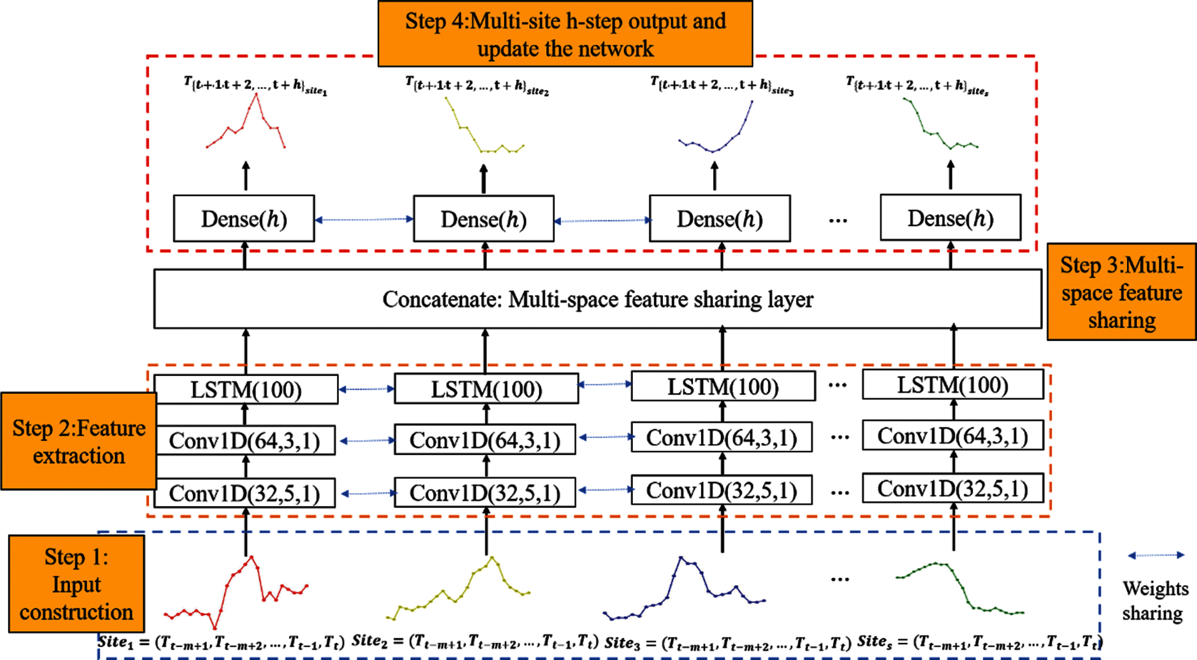
Figure 1: The proposed SCNN-LSTM for multi-site daily-ahead multi-step PM2.5 concentration forecasting

LabelSitei=|LabelSitei,1LabelSitei,2LabelSitei,3⋮LabelSitei,j⋮LabelSitei,M|=|Tm+1Tm+2⋯Tm+hTm+kTm+k+1⋯Tm+k+hTm+2k+1Tm+2k+1⋯Tm+2k+h⋮⋮⋮⋮Tt+1Tt+2⋯Tt+h⋮⋮⋮⋮Tm+(M−1)k+1Tm+(M−1)k+2⋯Tm+(M−1)k+h|(6)

{M+(M−1)k+h≤Nk≤mM=N−mk+1(7)

Input={[Site1,Site2,…,Sitei,…,Sites]}(8)

Output={[LabelSite1,LabelSite2,…,LabelSitei,…,LabelSites]}(9)

2.2.2 Feature Extraction

Due to the excellent feature extraction ability of CNN and the ability of LSTM to process time series with long-time dependency [27]. The proposed method adopts one-dimensional (1-D) CNN to extract short-time gap features, the extracted features are fed into LSTM to extract the features with long-time dependency. There are two sub-steps in the feature extraction part, as described following.

Short-time gap feature extraction: Two 1-D non-pooling CNN layers [28] are utilized to extract hidden features in the short-time gap as the PM2.5 series is relatively less-dimension. The process of 1-D convolution operation, as described in Eq. (10). Where the convoluted output x~ is calculated using (l−1)th's output xl−1 and Z filters with a bias bz, each filter is denoted as Kzl. After the convolution operation, the convoluted values are processed by one activation function f(⋅) to activate the feature maps. Significantly, Rectified Linear Unit (ReLU) could enhance feature expression ability by improving the nonlinear expression of the feature maps, which was applied in the proposed SCNN-LSTM, as shown in Eq. (11). By utilizing two 1-D CNN layers, sitei's short-time gap features sfsitei could be obtained, as defined in Eq. (12). Where Conv1D is a 1-D convolution operation in the format of Conv1D(filters, kernel_size, stride). Especially, the proposed method utilized 32, 64 as two layers’ filters and 5, 3 as the kernel size to extract the daily PM2.5 short-time gap features.

x~=f(xl−1×Kzl+bz),z∈Z(10)

f(x~)={x~,x~>00,otherwise(11)

{sfsite1=Conv1D(Conv1D(Site1))sfsite2=Conv1D(Conv1D(Site2))⋮sfsitei=Conv1D(Conv1D(Sitei))⋮sfsiten=Conv1D(Conv1D(Sites))(12)

LSTM feature extraction: Although CNN extracted short-time gap features, it loses some critical hidden patterns with long-time dependency. LSTM [29], a special RNN, could extract this kind of feature in a chain-like structure was utilized. The structure of LSTM, as shown in Fig. 2. Three cells existed in Fig. 2 over the time t−1, t, t+1. Three gate-like components in each LSTM cell, including input gate it, output gate ot,and forgot gate ft and control state Ct controlled the whole information flow. The calculations of LSTM's components at time t, as described in Eqs. (13)–(18).

it=σ(wi⋅[ht−1,sfsitei,t]+bi)(13)

ft=σ(wf⋅[ht−1,sfsitei,t]+bf)(14)

ot=σ(wo⋅[ht−1,sfsitei,t]+bo)(15)

Ct~=tanh(wc⋅[ht−1,sfsitei,t]+bc)(16)

Ct=ft∗Ct−1+it∗Ct~(17)

ht=ot∗tanh(Ct)(18)

where sfsitei,t is CNN extracted short-time gap features; wi,wf,wo,wc are connection weights of above three gates and cell state, and bi,bf,bo,bc are corresponding offset vectors; σ is activation function sigmoid and ∗ represents an element-wise calculation. The forgot gate decides what information from perceived hidden output ht−1 should be deleted according to current input sfsitei,t. In contrast, the dynamic states of the current cell are remembered by calculating Ct~. Moreover, the valuable part ft∗Ct−1 at the previous cell and new information it∗Ct~ will be added into the Ct. The hidden information ht is worked out according to the current stats Ct and output information ot, it reduces some meaningless information meanwhile adding some new useful knowledge over time as each site's final features for future PM2.5 forecasting. Thus, some unnormal information such as bad weather, holiday, big events could be remembered to enhance forecasting accuracy. Through s parallel LSTM layers, the short-time gap features with long-time dependency for each site could be obtained, as shown in Eq. (19). In which, each LSTM layer has 100 hidden nodes.

{featuresite1=LSTM(sfsite1)featuresite2=LSTM(sfsite2)⋮featuresitei=LSTM(sfsite3)⋮featuresites=LSTM(sfsites)(19)

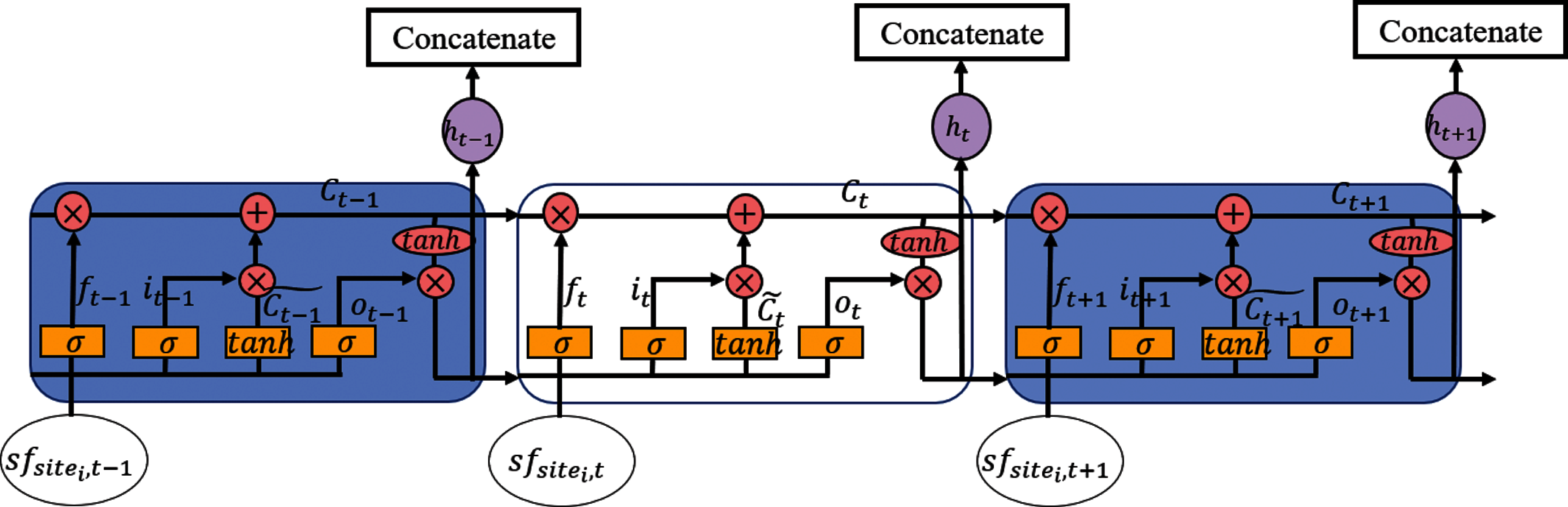
Figure 2: LSTM structure in the proposed SCNN-LSTM

2.2.3 Multi-space Feature Sharing

The space information is vital for PM2.5 forecasting as one space PM2.5 concentration is affected by adjacent spaces such as weather, environmental statues. To make full use of space information, the proposed method merged extracted s-site features from Eq. (19) as the fusion features to implement space sharing, as shown in Eq. (20). The fusion features contain short-time gap, long-time dependency, and space information are utilized for multi-site multi-step PM2.5 concentrations forecasting.

featuresfusion=Concatenate(featuresite1,featuresite2,…,featuresites)(20)

2.2.4 Multi-Site h-Step Output and Update the Network

The fusion features are utilized to forecast future s-site h-step PM2.5 concentrations in a linear mode. Each site's features contribute the same, implemented by one fully connected Dense layer with h nodes, as shown in Eq. (21). Moreover, multi-site outputs are implemented by the multiple loss functions, which is the key to achieve space-sharing through concatenate layer. It calculates the mean square error (MSE) between each site's ground truth and forecasting values to update the hidden layers and implement weights-sharing with a gradient descent algorithm. The total loss is the sum of s sites, as defined in Eq. (22). Each site contributes the same weight to the total loss.

{T{t+1,t+2,..,t+h}site1=Dense(featuresfusion)T{t+1,t+2,..,t+h}site2=Dense(featuresfusion)⋮T{t+1,t+2,..,t+h}sitei=Dense(featuresfusion)⋮T{t+1,t+2,..,t+h}sites=Dense(featuresfusion)(21)

Loss=1n(MSEsite1+MSEsite2+…+MSEsites)(22)

3  Experimental Verification

To validate the proposed method's effectiveness, the authors implement the proposed SCNN-LSTM based on the operating system of ubuntu 16.04.03, TensorFlow backend Keras. Moreover, the proposed method adopted “Adam” as the optimizer to find the best convergence path and “ReLu” as the activation function except the output layer is “linear.”

3.1 Data

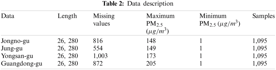
The authors adopted four real-word PM2.5 concentration data sets to validate the proposed method's effectiveness, including Jongno-gu, Jung-gu, Yongsan-gu, and Guangdong-gu from Seoul, South Korea, which is available on the website of http://data.seoul.go.kr/dataList/OA-15526/S/1/da-tasetView.do. Each data set is collected from 2017-01-01 00:00:00 to 2019-12-31 23:00:00. Noticed that some missing values caused by sensor failures or unnormal operations existed in each subset. The authors replaced them with the mean value of the nearest two values to reduce the influence of missing values. Then, we adopted Eqs. (5) and (6) to generate the input samples and the corresponding 10-step (h) labels in a sample rate m=24 and strides k=24. It means that we utilize 24-hour historical PM2.5 concentrations to forecast future 4-site daily-ahead 10-hour PM2.5 concentrations. Finally, we got four subsets with a length of 1,095=⌊26,28024⌋ samples. The more detailed information about the data, as described in Tab. 2.

3.2 Evaluation Metrics

We utilized multiple metrics including root mean square error (RMSE), mean absolute error (MAE), mean absolute percentage error (MAPE), and R square (R2) to evaluate the proposed method from multi-views. The calculation of each metric is given in Eqs. (23)–(26). Where yi is the ground truth of PM2.5 concentration at the time i, yi′ is the predicted value, y¯ is the meaning value of total y, and n is the number of samples.

RMSE=∑i=1n⁡(yi−yi′)2n(23)

MAE=1n∑i=1n⁡|yi−yi′|(24)

MAPE=100n∑i=1n⁡|yi′−yiyi|(25)

R2=1−∑i=1n(yi−yi′)2∑i=1n(yi−y¯)2(26)

3.3 Workflow

The workflow for multi-site and multi-step PM2.5 concentration forecasting using the proposed SCNN-LSTM, as shown in Fig. 3. Firstly, four-site historical series are normalized with Eq. (27) to reduce the influence of different units. Where T is PM2.5 series, ti is PM2.5 concentration at the time i, ti′ is normalized value. Then, utilizing Eqs. (5) and (6) to generate the corresponding input and output matrix. Thirdly, two-year (2017 and 2018) data are utilized for training the model, while the data in 2019 is for testing. In the training part, 20% of them are used to find the best model within minimum time with the early-stop strategy. Especially, we set patience as ten and epoch as 100. If the ‘val_loss’ does not decrease in ten epochs, the training process will be ended. The model with the lowest ‘val_loss’ will be saved as the best model. Otherwise, it will stop until 100 epochs. Lastly, the forecasting results are used to evaluate the model in terms of RMSE, MAE, MAPE, and R2.

ti′=ti−min(T)max(T)−min(T)(27)

3.4 Comparative Experiments

3.4.1 Multi-Step Forecasting

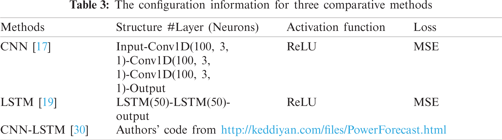
To validate the effectiveness and priority of the proposed method for daily-ahead multi-step PM2.5 concentration forecasting, we compared the proposed SCNN-LSTM with some leading deep learning methods, including CNN [17], LSTM [19], CNN-LSTM [30]. It is worth noticing that previous CNN and LSTM required additional meteorological or air pollutant factors; we use their structure for forecasting. The configurations of those comparative methods, as given in Tab. 3. Each comparative model runs four times for four-site forecasting, while the proposed method only needs to run once. The comparison results using averaged RMSE, MAE, MAPE, and R2 for four-site daily ahead 10-step PM2.5 concentration forecasting, as shown in Tab. 4. The findings indicated that the proposed method outperforms others, which won 13 times of 16 metrics on four subsets. Especially, the proposed method has an absolute priority at all evaluation metrics for all subsets compared to CNN. Although LSTM performs a little better than the proposed method at R2 on ‘Jongno-gu’ and MAE on ‘Jung-gu’. CNN-LSTM performs a little better than the proposed method at MAPE on ‘YongSan-gu.’ They require to run various times to get the forecasting results for each site while the proposed method only needs to run once. Moreover, the standard error proved the proposed method has good robustness. The performance of each method is ranked as: Proposed > CNN-LSTM > LSTM > CNN by comparing the averaged evaluation metrics on four sites. Especially, the proposed method has an averaged MAPE of 23.96% with a standard error of 1.94%, while others are greater than 25%, and only the proposed method's R2 is more significant than 0.7. Besides, we found CNN could not forecast multi-step PM2.5 concentration well due to all MAPE are greater than 100% (that is not caused by a division by zero error). The forecasting results for different methods, as shown in Fig. 4. The findings indicated that only the proposed method could accurately forecast PM2.5 concentration's trend and value while others cannot. Also, Fig. 4 shows long-step forecasting is more complicated than short-step. In summary, the proposed SCNN-LSTM could accurately, effectively, and expediently forecast multi-site daily-ahead multi-step PM2.5 concentrations.

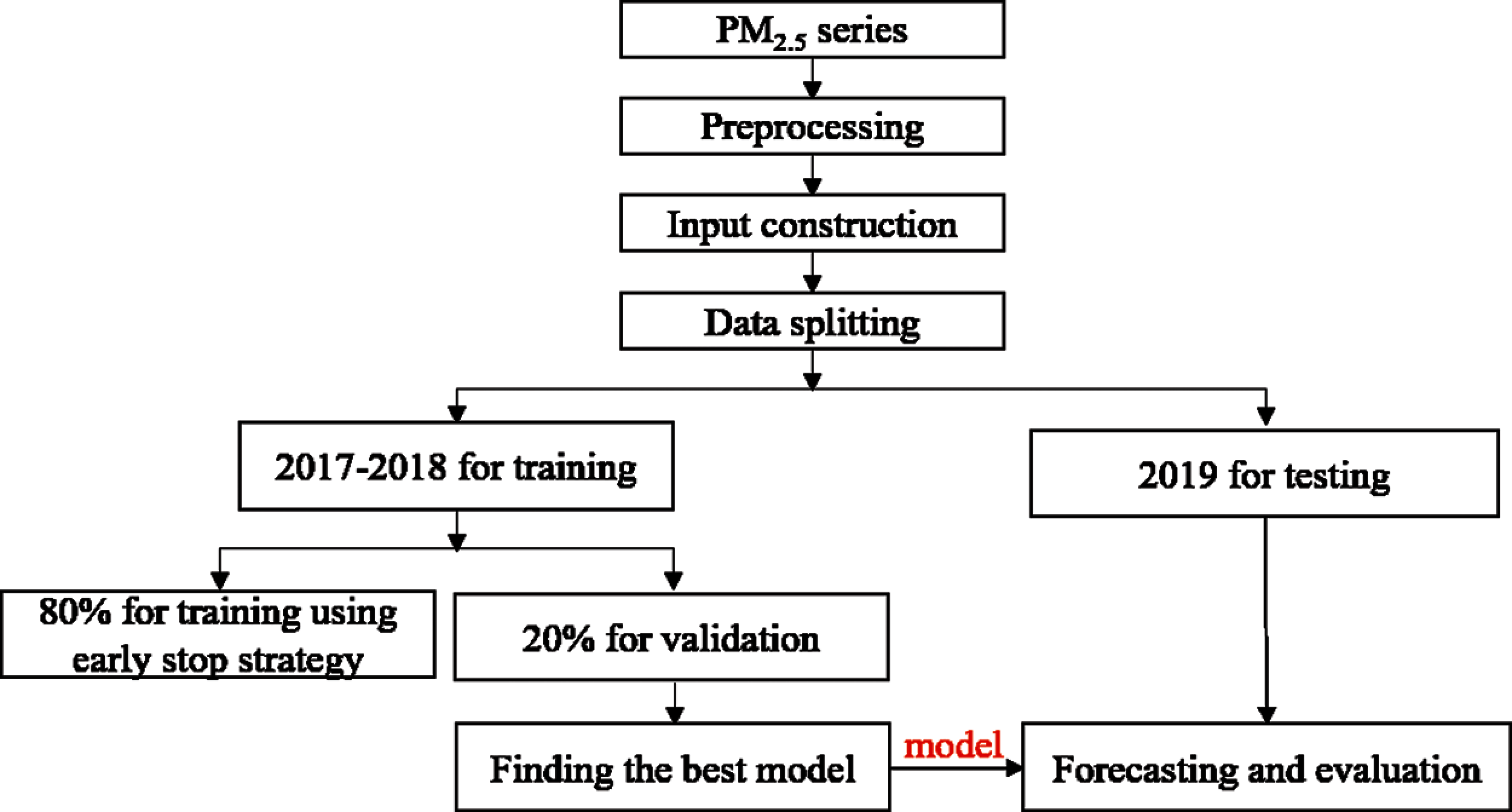
Figure 3: The workflow for multi-site and multi-step PM2.5 concentration forecasting

3.4.2 Each-step Forecasting

To explore and verify the effectiveness of the proposed method for each-step PM2.5 forecasting, we calculated averaged RMSE, MAE, MAPE, and R2 for each step on four sites using the above deep models except CNN as its MAPE does not make sense. The comparison results showed that the proposed method has an absolute advantage for each step forecasting on all evaluation metrics, which could be conducted from Fig. 5. Especially, the proposed method has the lowest RMSE and R2 for each-step forecasting. For MAE, the proposed method has the lowest values except for the third step is a little greater than LSTM. The MAPE indicated that the proposed method performs very well on the first five-step forecasting. Especially, the first three steps’ MAPE is lower than 20%, which improves a lot compared to the other two methods. R2 indicated that the proposed method could explain more than 97% for the first step, 92% for the second step. Moreover, the results indicated that the forecasting performance decreases with the steps. Significantly, the relationship between each evaluation metric and the forecasting step for the proposed method is denoted as Eqs. (28)–(31). It shows that if increasing one step, the RMSE will increase by 0.6588, MAE will increase by 0.4890, MAPE will increase by 2.2174, while R2 will decrease by 0.0595, respectively.

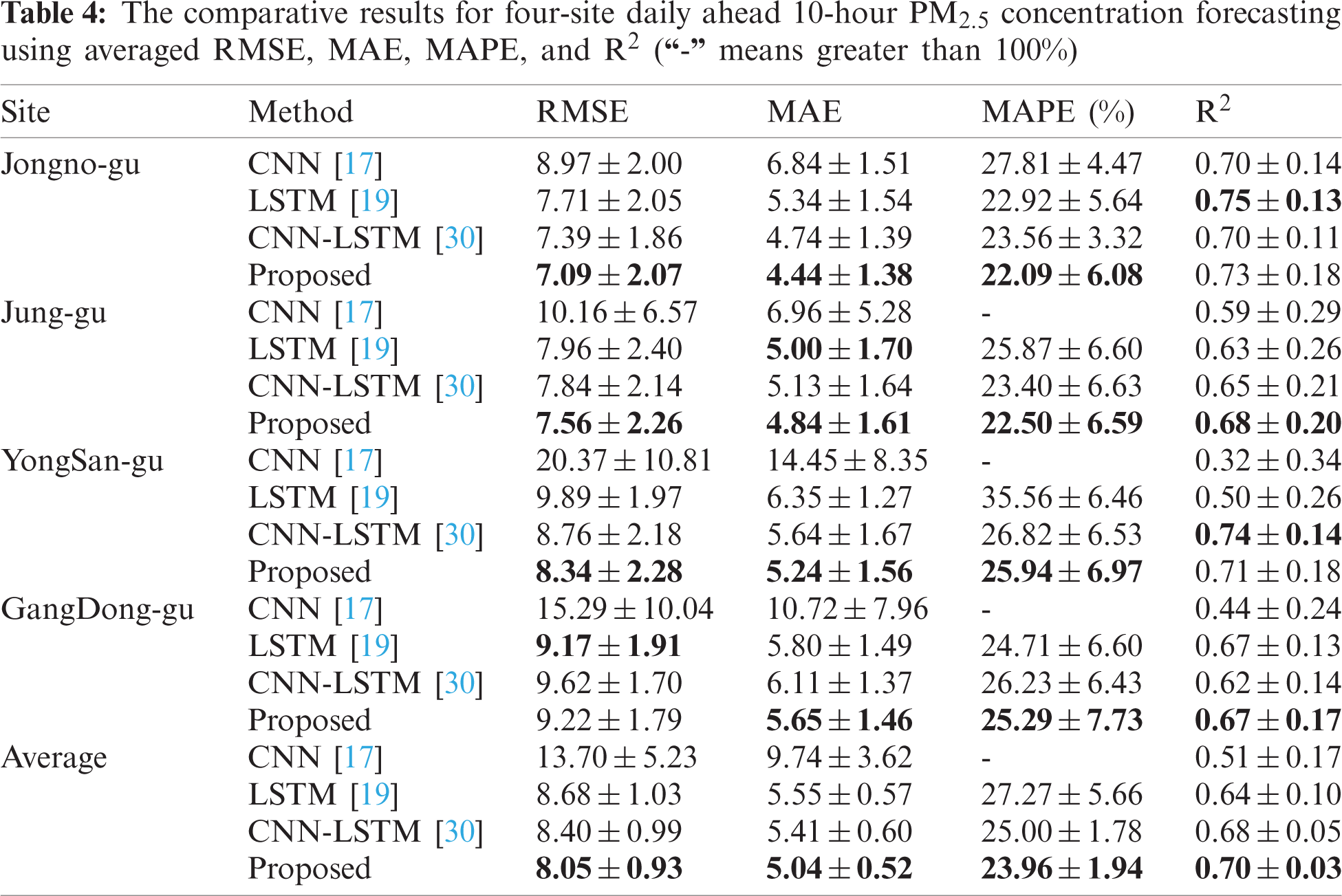
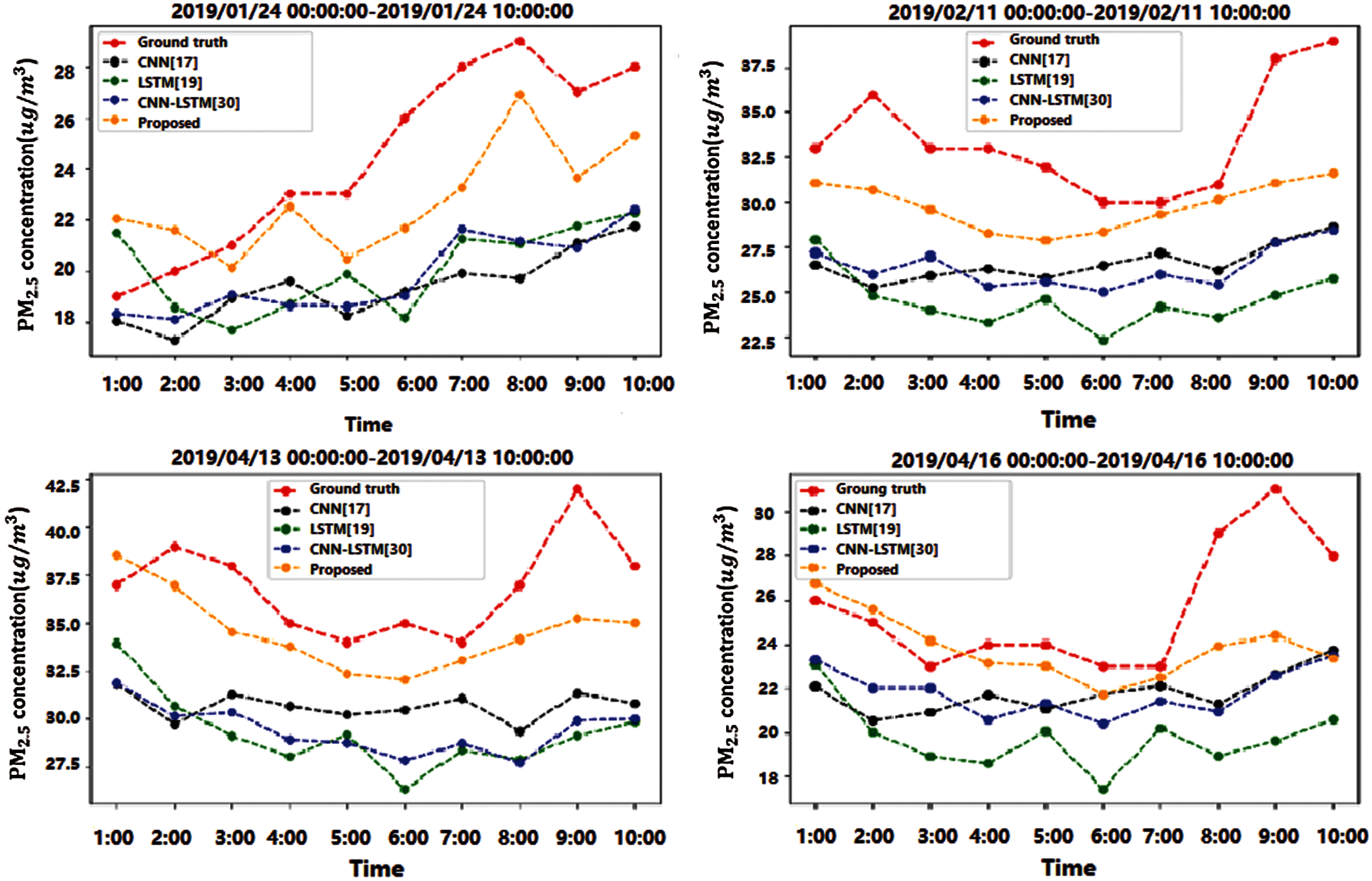
Figure 4: The forecasting results using different methods

RMSE=0.6588⋅step+4.43(28)

MAE=0.4890⋅step+2.35(29)

MAPE=2.2174⋅step+11.76(30)

R2=−0.0595⋅step+1.03(31)

3.5 Ablation Study

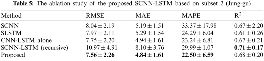
To explore each part's effectiveness in the proposed SCNN-LSTM, we designed four sub-experiments. Specially, designed space-shared CNN (SCNN) to verify the effectiveness of LSTM; Designed space-shared LSTM to verify the effectiveness of CNN; and designed CNN-LSTM without a space-shared mechanism (CNN-LSTM alone) to verify its effectiveness; designed SCNN-LSTM with a recursive strategy to validate the effectiveness of the multi-output strategy. All configurations of those methods are the same as the proposed method. The results based on subset 2 (Jung-gu), as shown in Tab. 5.

The results indicated that the utilization of LSTM had improved RMSE by 5.97%, MAE by 6.74%, MAPE by 32.57%, and R2 by 1.49%, which conducts by comparing SCNN and the proposed method. The application of CNN has improved 5.14% of RMSE, 8.51% of MAE, 7.37% of MAPE, and 10.29% of R2. By comparing the CNN-LSTM alone with the proposed method, we can conduct that the space-shared mechanism has improved 2.45% of RMSE, 2.02% of MAE, 3.18% of MAPE, and 1.49% of R2. Moreover, by comparing the SCNN-LSTM with a recursive strategy to the proposed method, the findings derived that the multi-output strategy has absolute priorities as it performs much better on RMSE, MAE, and MAPE except for R2 is a little worse. In summary, the above evidence proved that CNN could extract the short-time gap feature; LSTM could mine hidden features which have a long-time dependency; The space-shared mechanism ensures full utilization of space information; The multi-output strategy could save training cost simultaneously keeping high forecasting accuracy. Combining those parts properly could accurately forecast the multi-site and multi-step PM2.5 concentrations only using self-historical series and running once.

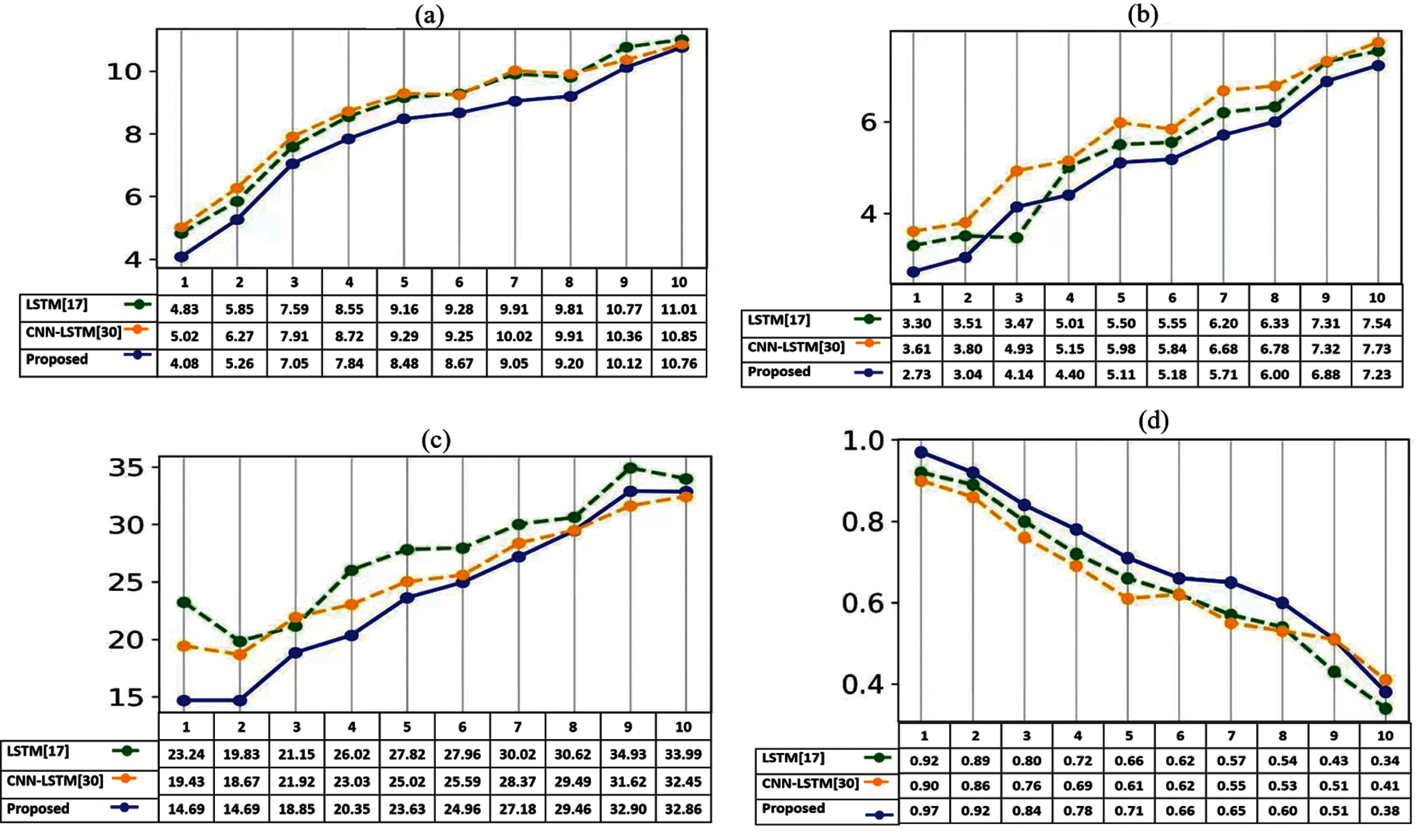
Figure 5: Averaged metrics for each step forecasting on four sites: (a) RMSE, (b) MAE, (c) MAPE, and (d) R2

4  Discussion

We have proposed a novel SCNN-LSTM deep model to extract the rich hidden features from multi-site self-historical PM2.5 concentration series for multi-site daily-ahead multi-step PM2.5 concentration forecasting, as shown in Fig. 1. It contains multi-channel inputs and outputs corresponding to multi-site inputs and future outputs. Each site's self-historical series is fed into CNN-LSTM to extract short-time gap and long-time dependency individually first, then extracted features are merged as the final features to forecast multi-site daily-ahead multi-step PM2.5 concentrations.

To validate the proposed method's effectiveness, we compared it with three leading deep learning methods, including CNN, LSTM, and CNN-LSTM, on four real-word PM2.5 data sets from Seoul, South Korea. The comparative results indicated that the proposed SCNN-LSTM outperforms others in terms of averaged RMSE, MAE, MAPE, and R2, which could be conducted from Tab. 4. Especially, the proposed method got averaged RMSE, MAE, MAPE, and R2 are 8.05%, 5.04%, 23.96%, and 0.70 on four data sets. Fig. 4 confirmed its excellent forecasting performance again and showed the long-step forecasting is more changeling and difficult than short-step. Also, the proposed method has good robustness, which could be conducted from Tab. 4 by using standard error.

Moreover, the authors have explored the proposed method's effectiveness for each-step forecasting, as shown in Fig. 5. The comparison results showed that the proposed method has an absolute advantage for each step forecasting on all evaluation metrics. Also, the relationship between each evaluation metric and the forecasting step has been conducted at Eqs. (28)–(31). It shows that if the forecasting step increases one, the RMSE will increase 0.6588, MAE will increase 0.4890, MAPE will increase 2.2174, while R2 will decrease 0.0595, respectively.

To validate each component's effectiveness, an ablation study is done, as described in Tab. 5. The results indicate that CNN could extract the short-time gap feature; LSTM could mine hidden features which have a long-time dependency; The space-shared mechanism ensures full utilization of space information; The multi-output strategy could save training cost simultaneously keeping high forecasting accuracy, respectively.

By setting the parameters of the proposed SCNN-LSTM, the forecasting accuracy could improve. Future studies will focus on using deep reinforcement learning technology to find the best parameter under the structure of the proposed SCNN-LSTM.

5  Conclusions

This manuscript has developed an accurate, convenient framework based on CNN and LSTM for multi-site daily-ahead multi-step PM2.5 concentration forecasting. In which, CNN is used to extract the short-time gap features; CNN extracted hidden features are fed into LSTM to mine hidden patterns with a long-time dependency; Each site's hidden features extracted from CNN-LSTM are merged as the final features for future multi-step PM2.5 concentration forecasting. Moreover, the space-shared mechanism is implemented by multi-loss functions to achieve space information sharing. Thus, the final features are the fusion of short-time gap, long-time dependency, and space information, which is the key to ensure accurate forecasting. Besides, the usage of the multi-output strategy could save training costs simultaneously keep high forecasting accuracy. The sufficient experiments have confirmed its state-of-the-art performance. In summary, the proposed SCNN-LSTM could forecast multi-site daily-ahead multi-step PM2.5 concentrations only by using self-historical series and running once.

Funding Statement: This work was supported by a Research Grant from Pukyong National University (2021).

Conflicts of Interest: The authors declare that they have no conflicts of interest to report regarding the present study.

References

 1.  S. Ausati and J. Amanollahi, “Assessing the accuracy of ANFIS, EEMD-GRNN, PCR, and MLR models in predicting PM2.5,” Atmospheric Environment, vol. 142, pp. 465–474, 2016.

 2.  W. Sun and J. Sun, “Daily PM2.5 concentration prediction based on principal component analysis and LSSVM optimized by cuckoo search algorithm,” Journal of Environmental Management, vol. 188, pp. 144–152, 2017.

 3.  W. Sun and Z. Li, “Hourly PM2.5 concentration forecasting based on feature extraction and stacking-driven ensemble model for the winter of the Beijing-Tianjin-Hebei area,” Atmospheric Pollution Research, vol. 11, no. 6, pp. 110–121, 2020.

 4.  R. Zhao, X. Gu, B. Xue, J. Zhang and W. Ren, “Short period PM2.5 prediction based on multivariate linear regression model,” PLOS ONE, vol. 13, no. 7, pp. 1–15, 2018.

 5.  A. Z. Ul-Saufie, A. S. Yahaya, N. A. Ramli, N. Rosaida and H. A. Hamid, “Future daily PM10 concentrations prediction by combining regression models and feedforward backpropagation models with principle component analysis (PCA),” Atmospheric Environment, vol. 77, pp. 621–630, 2013.

 6.  P. J. García Nieto, F. Sánchez Lasheras, E. García-Gonzalo and F. J. de Cos Juez, “PM10 concentration forecasting in the metropolitan area of oviedo (Northern Spain) using models based on SVM, MLP, VARMA and ARIMA: A case study,” Science of the Total Environment, vol. 621, pp. 753–761, 2018.

 7.  Y. Cheng, H. Zhang, Z. Liu, L. Chen and P. Wang, “Hybrid algorithm for short-term forecasting of PM2.5 in China,” Atmospheric Environment, vol. 200, no. December 2018, pp. 264–279, 2019.

 8.  X. Shao, C. -S. Kim and P. Sontakke, “Accurate deep model for electricity consumption forecasting using multi-channel and multi-scale feature fusion CNN–LSTM,” Energies, vol. 13, no. 8, pp. 1881, 2020.

 9.  J. K. Deters, R. Zalakeviciute, M. Gonzalez and Y. Rybarczyk, “Modeling PM2.5 urban pollution using machine learning and selected meteorological parameters,” Journal of Electrical and Computer Engineering, vol. 2017, pp. 5106045, 2017.

10. H. J. S. Fernando, M. C. Mammarella, G. Grandoni, P. Fedele, R. Marco et al., “Forecasting PM10 in metropolitan areas: Efficacy of neural networks,” Environmental Pollution, vol. 163, pp. 62–67, 2012.

11. H. Liu, K. Jin and Z. Duan, “Air PM2.5 concentration multi-step forecasting using a new hybrid modeling method: Comparing cases for four cities in China,” Atmospheric Pollution Research, vol. 10, no. 5, pp. 1588–1600, 2019.

12. X. Shao, C. Pu, Y. Zhang and C. S. Kim, “Domain fusion CNN-lSTM for short-term power consumption forecasting,” IEEE Access, vol. 8, pp. 188352–188362, 2020.

13. Y. Weng, X. Wang, J. Hua, H. Wang, M. Kang et al., “Forecasting horticultural products price using ARIMA model and neural network based on a large-scale data set collected by web crawler,” IEEE Transactions on Computational Social Systems, vol. 6, no. 3, pp. 547–553, 2019.

14. Y. Lecun, Y. Bengio and G. Hinton, “Deep learning,” Nature, vol. 521, no. 7553, pp. 436–444, 2015.

15. S. Hochreiter and J. Schmidhuber, “Long short-term memory,” Neural Computation, vol. 9, no. 8, pp. 1735–1780, 1997.

16. J. Xie, “Deep neural network for PM2.5 pollution forecasting based on manifold learning,” in Proc. SDPC, Shanghai, SH, China, pp. 236–240, 2017.

17. P. Y. Kow, Y. S. Wang, Y. Zhou, L. F. Kao, M. Lssermann et al., “Seamless integration of convolutional and back-propagation neural networks for regional multi-step-ahead PM2.5 forecasting,” Journal of Cleaner Production, vol. 261, pp. 121285, 2020.

18. Y. Park, B. Kwon, J. Heo, X. Hu, Y. Liu et al., “Estimating PM2.5 concentration of the conterminous United States via interpretable convolutional neural networks,” Environmental Pollution, vol. 256, pp. 113395, 2020.

19. Y. A. Ayturan, Z. C. Ayturan, H. O. Altun, C. Kongoll, F. D. Tuncez et al., “Short-term prediction of PM2.5 pollution with deep learning methods,” Global Nest Journal, vol. 22, no. 1, pp. 126–131, 2020.

20. Z. Zhang, Y. Zeng and K. Yan, “A hybrid deep learning technology for PM2.5 air quality forecasting,” Environmental Science and Pollution Research, vol. 28, pp. 39409–39422, 2021. [Online]. Available: http://www.globalbuddhism.org/jgb/index.php/jgb/article/view/88/100.

21. D. Qin, J. Yu, G. Zou, R. Yong, Q. Zhao et al., “A novel combined prediction scheme based on CNN and LSTM for urban PM2.5 concentration,” IEEE Access, vol. 7, pp. 20050–20059, 2019.

22. Y. Qi, Q. Li, H. Karimian and D. Liu, “A hybrid model for spatiotemporal forecasting of PM2.5 based on graph convolutional neural network and long short-term memory,” Science of the Total Environment, vol. 664, pp. 1–10, 2019.

23. U. Pak, J. Ma, U. Ryu, K. Ryom, U. Juhyok et al., “Deep learning-based PM2.5 prediction considering the spatiotemporal correlations: A case study of Beijing, China,” Science of the Total Environment, vol. 699, pp. 133561, 2020.

24. A. P. K. Tai, L. J. Mickley and D. J. Jacob, “Correlations between fine particulate matter (PM2.5) and meteorological variables in the United States: Implications for the sensitivity of PM2.5 to climate change,” Atmospheric Environment, vol. 44, no. 32, pp. 3976–3984, 2010.

25. C. D. Whiteman, S. W. Hoch, J. D. Horel and A. Charland, “Relationship between particulate air pollution and meteorological variables in Utah's Salt Lake Valley,” Atmospheric Environment, vol. 94, pp. 742–753, 2014.

26. J. C. S. Shamsul Masum and Y. Liu, “Multi-step time series forecasting of electric load using machine learning models,” in Proc. ICAISC 2018, Zakopane, Poland, vol. 1, pp. 148–159, 2018.

27. L. Ren, J. Dong, X. Wang, Z. Meng, L. Zhao et al., “A data-driven auto-cNN-lSTM prediction model for lithium-ion battery remaining useful life,” IEEE Transactions on Industrial Informatics, vol. 17, no. 5, pp. 3478–3487, 2021.

28. S. Liu, H. Ji and M. C. Wang, “Nonpooling convolutional neural network forecasting for seasonal time series with trends,” IEEE Transactions on Neural Networks and Learning Systems, vol. 31, no. 8, pp. 2827–2888, 2020.

29. S. Hochreiter and J. U. Schmidhuber, “Long short-term memory,” Neural Computation, vol. 9, no. 8, pp. 1735–1780, 1997.

30. K. Yan, X. Wang, Y. Du, N. Jin, H. Huang et al., “Multi-step short-term power consumption forecasting with a hybrid deep learning strategy,” Energies, vol. 11, no. 11, pp. 3089, 2018.

This work is licensed under a Creative Commons Attribution 4.0 International License, which permits unrestricted use, distribution, and reproduction in any medium, provided the original work is properly cited.