DOI:10.32604/cmc.2022.020495

| Computers, Materials & Continua DOI:10.32604/cmc.2022.020495 |  |
| Article |
Deep Learning Based Modeling of Groundwater Storage Change
1College of Computer and Information Sciences Majmaah University Almajmaah, 11952, Saudi Arabia
2CHRIST (Deemed to be University), Bangalore, India
*Corresponding Author: Mohd Anul Haq. Email: m.anul@mu.edu.sa
Received: 26 May 2021; Accepted: 03 July 2021
Abstract: The understanding of water resource changes and a proper projection of their future availability are necessary elements of sustainable water planning. Monitoring GWS change and future water resource availability are crucial, especially under changing climatic conditions. Traditional methods for in situ groundwater well measurement are a significant challenge due to data unavailability. The present investigation utilized the Long Short Term Memory (LSTM) networks to monitor and forecast Terrestrial Water Storage Change (TWSC) and Ground Water Storage Change (GWSC) based on Gravity Recovery and Climate Experiment (GRACE) datasets from 2003–2025 for five basins of Saudi Arabia. An attempt has been made to assess the effects of rainfall, water used, and net budget modeling of groundwater. Analysis of GRACE-derived TWSC and GWSC estimates indicates that all five basins show depletion of water from 2003–2020 with a rate ranging from −5.88 ± 1.2 mm/year to −14.12 ± 1.2 mm/year and −3.5 ± 1.5 to −10.7 ± 1.5, respectively. Forecasting based on the developed LSTM model indicates that the investigated basins are likely to experience serious water depletion at rates ranging from −7.78 ± 1.2 to −15.6 ± 1.2 for TWSC and −4.97 ± 1.5 to −12.21 ± 1.5 for GWSC from 2020–2025. An interesting observation was a minor increase in rainfall during the study period for three basins.
Keywords: LSTM; forecasting; time series; tensorflow; keras; modeling
The arid and semi-arid regions of the world have historically suffered from depleting freshwater resources, including TWS (Terrestrial Water Storage) and GWS (Ground Water Storage), apart from low rainfall and rising water demands. The depletion of these water resources primarily depends on climatic parameters (precipitation and temperature) and the rising water demand for municipal, agricultural and industrial purposes. The population of Saudi Arabia increased by 15.48% from 27.4 million in 2010 to 32.4 million in 2016, and the volume of extracted groundwater also rose by 27% from 15.8 × 10⁹ cubic meters in 2010 to 21.6 × 10⁹ cubic meters in 2016 [1]. Monitoring GWS change and future water resource availability are crucial, especially in arid areas like Saudi Arabia. Traditional methods such as in situ well measurement for monitoring GWS are immensely challenging due to data unavailability [1–3].
The GRACE satellite missions provide an excellent opportunity to monitor TWS and GWS [4]. GRACE data has been used successfully to estimate GWSC worldwide, such as in Africa [5–7], northwestern India [2,8–10], in the United States [11,12] in Australia [13], in the Middle East [14–18] and in China [2,18–20]. Saudi Arabia has also shown evidence of water resource exploitation and severe groundwater decline by recent studies using the GRACE dataset from 2002 to 2016 [15,17,18,21,22].
The present investigation also contributes to two major aspects: forecasting the future status of GWSC using LSTM modeling from July 2020 to December 2025 and analyzing the correlation between groundwater change and rainfall. There are four main objectives of the present investigation: (1) to analyze the changes in TWSC and GWSC from 2003–2020, (2) to analyze the relationships among TWSC, GWSC, satellite-based rainfall and rainfall from meteorological stations from 2009 to 2016; (3) to estimate the net budget modeling of groundwater based on GWSC and rainfall; and (4) to forecast TWSC and GWSC changes from July 2020 to June 2025 using developed and tuned LSTM models. All these objectives were accomplished for entire Saudi Arabia and five basins within Saudi Arabia. A total of 364 tiles of SRTMGL3 DEM were downloaded from LPDAAC (https://lpdaac.usgs.gov) to prepare the entire KSA mosaic (Fig. 1).
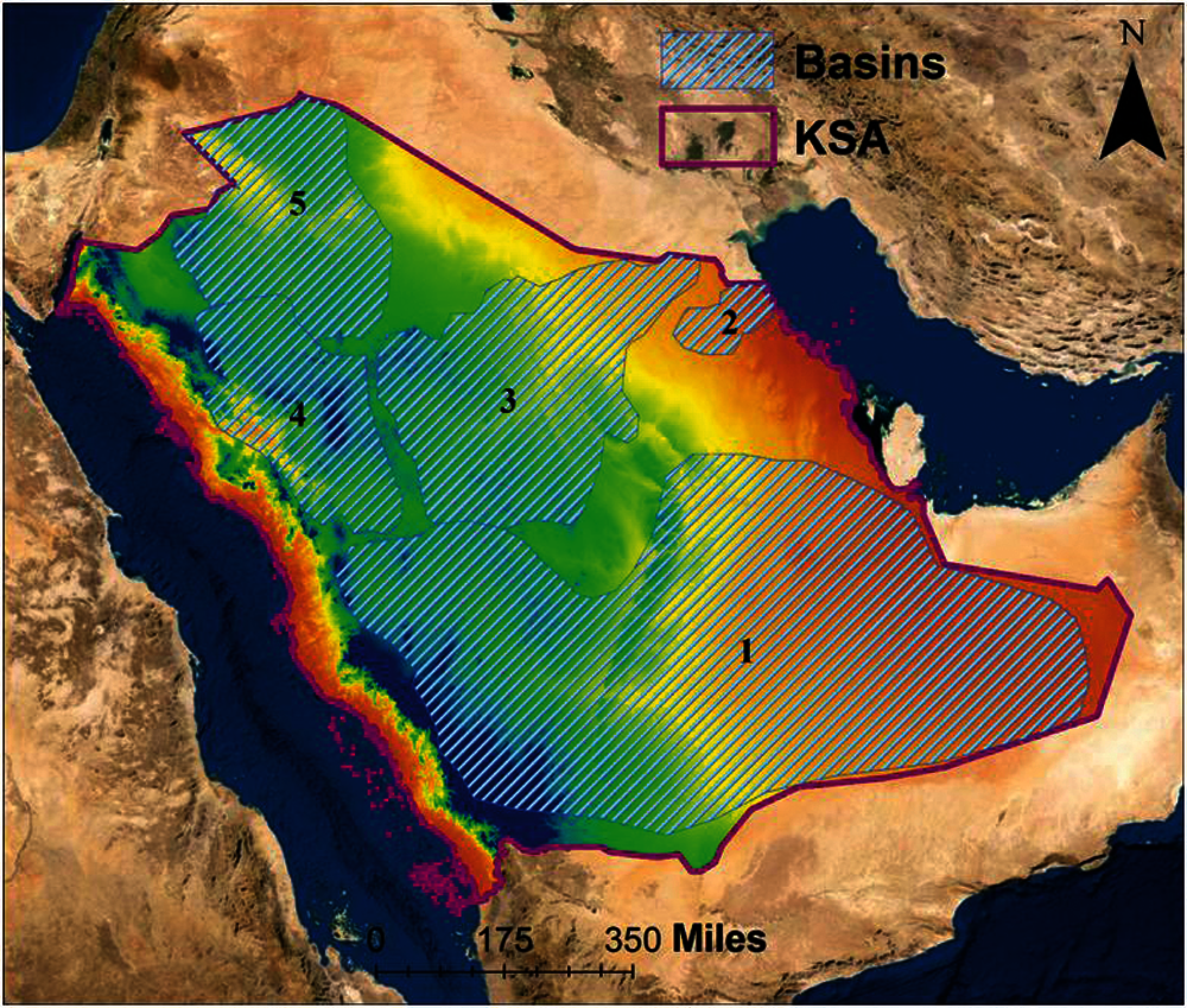
Figure 1: Map of KSA with mosaicked SRTM DEM background
LSTM networks are a type of RNN that use special units (cells) and standard units to overcome the limitation of traditional RNN [23–26]. There are three gates, which are contained by a cell in LSTM. The first gate is the input gate, the second is termed as the forget gate, whereas the third is the output gate. The LSTM network composition function's description is based on the input node, and the three gates are contained by a cell, cell state and output layer. Eqs. (1)–(7) are as follows [27,28].
Input node
Input gate
Forget gate
Output gate
Cell state
Hidden gate
Output layer
Recent studies have used LSTM models [29–35], ML models [36–39] and ANN models [40,41] to forecast groundwater level (GWL). Earlier investigations have forecasted the GWL within the time series of observed data while others have forecasted for three months [36]. The scope of the present study entails forecasting the values within time series. Also, this study's novelty lies in the evaluation and tuning of the LSTM models to forecast the future TWSC and GWSC for 65-timesteps (monthly) from July 2020 to December 2025. We could have forecasted for a longer time range, but it was deemed infeasible due to the size of historical time series data (2003–2020). This study is almost certainly the first investigation that reports GRACE forecasting-derived TWS and GWS using LSTM modeling for entire Saudi Arabia.
Terrestrial water storage (TWS) was obtained from GRACE and GRACE-FO satellites. These satellite missions were jointly launched by NASA (https://grace.jpl.nasa.gov/data/get-data/) and the German Aerospace Centre (DLR). GRACE and GRACE-FO information from January 2003 to June 2020 were obtained at 0.5° spatial resolution and monthly temporal resolutions. There was no GRACE satellite coverage from July 2017 to May 2018, and data gaps occurred from August 2018 to September 2018. Therefore, the years 2017–2018 were excluded from the present investigation. GRACE release 06 (RL06) V 2.0 global mass concentration blocks or mascon products were used in the present investigation, which were acquired from Jet Propulsion Laboratories (JPL). The primary reason to choose the JPL product over other products was the absence of leakage and measurement uncertainties [42,43].
The monthly rainfall dataset of Saudi Arabia from January 2009 to December 2018 was procured from the General Authority for Statistics [1]. This dataset contained rainfall (in mm) from 26 PME MET Stations without significant gaps. The Tropical Rainfall Measuring Mission (TRMM) data was procured from January 2009 until December 2014, and Global Precipitation Measurement (GPM) data was procured from January 2015 to November 2020 from NASA's Precipitation Processing System (https://pps.gsfc.nasa.gov/). The precipitation data of MET stations and precipitation data from TRMM and GPM's satellite mission have been abbreviated as METRain and SatRain, respectively.
3.1 GRACE TWS and GWS Estimation
TWS was estimated using GRACE and GRACE-FO satellites from Jan 2003 to June 2020 at 0.5° spatial and monthly temporal resolutions. GRACE, on its own, is incapable of separating anomalies from several elements of TWS (e.g., surface water storage, canopy water, and soil moisture content). Therefore, it is essential to subtract non-groundwater components. When this process is carried out for TWS data, the GWS can be obtained. The current study area being the arid and semi-arid part of Saudi Arabia, the contribution of surface water storage and canopy water was likely to be insignificant in the overall calculation. However, the soil moisture content (SMC) had to be subtracted from the change in TWS (TWSC) to get the change in GWS (GWSC), see Eq. (8).
In the equation, GWSC and SMCC showed changes in groundwater storage and changes in soil moisture content, respectively. Information related to soil moisture was obtained using the Global Land Data Assimilation System (GLDAS) [44,45]. The GRACE TWS data was re-gridded to 1° to make the resolutions identical to GLDAS-modeled data based on the approach of [46]. The GLDAS-modeled data were chosen over other LSMs since it provides practical approximation related to the soil moisture content in arid areas [17]. Since the difference between GLDAS models can cause uncertainty in GWS estimates, the ensemble mean of GWS was estimated based on the three LSMs for our analysis.
3.2 GRACE TWSC and GWSC Uncertainty Estimation
The calculation of total TWSC uncertainties (∂TWSC) was performed using the methodology described by [17,47]. TWSC annual and semi-annual trends and first residual (r1) were calculated. The lag value of 13 months was used to remove the annual trend from the time series and second residual (r2), and its standard deviation (r3) was calculated. The values of r1, r2, and r3 were added to get the total uncertainty from the TWSC. The uncertainty in SMCC (∂SMCC) was estimated as the mean monthly standard deviation from the three GLDAS models [21,46,47]. The total uncertainty in the GWSC (∂GWSC) was calculated using quadratic addition related to TWSC and SMCC values, see Eq. (9).
Mann-Kendall tests [48,49] were carried out for trend analysis to detect trends and changes in GWSC over the years of analysis. Sen's slope values [50] were used to understand the trend of GWSC change for five sub-basins of KSA from Jan 2003 to June 2020. Statistics of Mann-Kendall S value [48,49] were evaluated for chronologically placed observations in the time series Eq. (10). The variance of the observations VAR(S) in the time series was also estimated as per Eq. (12). Standardized test Z Eq. (13) [51] for the statistical analyses was also performed.
Here,
3.4 Correlation Analysis Between Variables
An attempt was made to study the correlation analysis among GWSC, TWSC, SatRain and METRain for five basins from Jan 2009 to Dec 2016 as per the availability of a common temporal dataset [15]. compared the mean values of rainfall each month, obtained using records of rain gauges and global weather data, and reported correlation coefficients ranging from 0.72 to 0.85. We have used SatRain and METRain for correlation analysis for all five basins. A significant association between the records of SatRain and METRain cannot be anticipated as SatRain corresponds to measurements over significantly wide-ranging areas (0.5o × 0.5o).
3.5 Data Pre-Processing for LSTM-Based Forecasting
Data transformation is crucial before implementing the LSTM model. Three data transformations were applied in the current investigation. First, a lag variable of 1 was applied to remove the decreasing trend in the dataset. The second step was the transformation of time series data into input and output so that the output of a step becomes the input of the next step to forecast the value of the current time step. As described earlier, total data in the time series were 186 monthly values. The first 150 months’ dataset for all five basins were taken for the training (126 months) and testing (24 months) of the LSTM model; the remaining 36 months of data (July 2015-June 2020, data gaps of 2016 and 2017) were kept separate from the training process for the unbiased external validation of the LSTM prediction. The third transformation was the scaling of time series data from −1 to 1. All these three transformations were inverted after the prediction step to get the values at the original scale so that the uncertainty calculation could be adequately assessed.
3.6 Implementation of LSTM Model
Keras library version 2.3.0 with TensorFlow version 2.0 at the backend and Python version 3.8.0 was used to build the LSTM models in the current study. The libraries used in the current investigation were NumPy, Pandas, Matplotlib, and scikit-learn. A 4 step procedure was applied to implement LSTM.
The first step was to define the LSTM network, which is organized as a sequence of layers contained by a sequential model. LSTM layer requires that the number of inputs in a three-dimensional shape consists of samples, time steps and features; therefore, reshape function was used to convert our data into a three-dimensional shape based on 130 samples of training, monthly time-step, and features represented by five basins. Two LSTM layers were used in the current investigation. In the first LSTM layer, the return_sequences were set to true, and it indicated that the output of each neuron's hidden state was used as an input to the next LSTM layer. Several hyper-parameters such as optimizer, learning rate, number of units, momentum, and activation functions have to be chosen a priori. Activation functions are required for functional mapping of an input value to an output signal; now, this output becomes the input in the next layer. The dropout layer was added between two LSTM layers, and outputs of the prior layer were fed to the subsequent layer to prevent overfitting. It works by “dropping out” or probabilistically removing inputs to a layer, which may be input variables from a previous layer. The reason to choose dropout over L1 and L2 regularization was that dropout provides regularization, including robustness to the network, allowing it to evaluate different networks. It has a float value between 0 and 1 with a default value of 1. A value of 0.5 was chosen with two dropout layers.
The second step was compiling the network. It required several parameters, such as an optimization algorithm to train the network and the loss function to evaluate the network. Several optimizers were tested based on their performances. The third step was the fitting of the LSTM model. The objective of model fitting is to adapt the weights based on a training dataset. It requires the training data to be specified for inputs and corresponding outputs. The initial value of epochs was given as 100 with a validation split value of 0.2 (i.e., 30 values for internal validation of the model) and input and output values.
The fourth and essential step was the prediction using the LSTM model. We forecasted the output step by step for the test data, and the model fed the current forecasted value back into the input window by moving it one step forward to aid forecasting at the next time step using the moving-forward window technique [23]. Here we used a moving forward window of size 24, which means we used the first 24 data inputs to forecast the 25th data point. Next, we used the window between 1 to 25 data inputs to forecast the 26th data point and so on. We used the pandas shift function that shifts the entire column by the specified number for moving the window. In this, we shifted the column up by one and then concatenated that to the actual data. After fixing the window's size, the 25th column in the table becomes the target y, and the first 24 columns become our input x1, x2,…, x24 features. Using this method, we forecasted the GWSC individually for 36 months from July 2015-June 2020 (data gaps of 2016 and 2017), or three years. As mentioned earlier, the model prediction's external evaluation was based on a separate dataset of 36-time steps data that had been kept separate from the training and testing months.
Tuning the hyper-parameters of any neural network model is essential for evaluating and appraising the model. The major hyper-parameters of LSTM tuned in the present investigation were (1) number of nodes, (2) number of training epochs, (3) choice of optimizer, and (4) learning rate. A walk-forward model evaluation using the hyper-parameters mentioned above was attempted for different configuration values. The prediction on the test dataset was evaluated based on root mean squared error (RMSE).
The first configuration tuned was based on the number of nodes, which influences the learning capability of the LSTM model. Generally, more nodes can learn more complex mapping at the cost of training time and sometimes cause overfitting. Different nodes (1, 2, 4, 6, and 8) were tested for different configurations. By using four numbers of nodes, a lesser average RMSE value of 1.4 and the least variance based on 20 experimental runs were obtained. However, since it could be an indication of overfitting, dropout was applied to prevent overfitting. The box and whisker plot (Fig. 2A) suggested that eight nodes showed an average RMSE value of 1.85 and the highest variance.
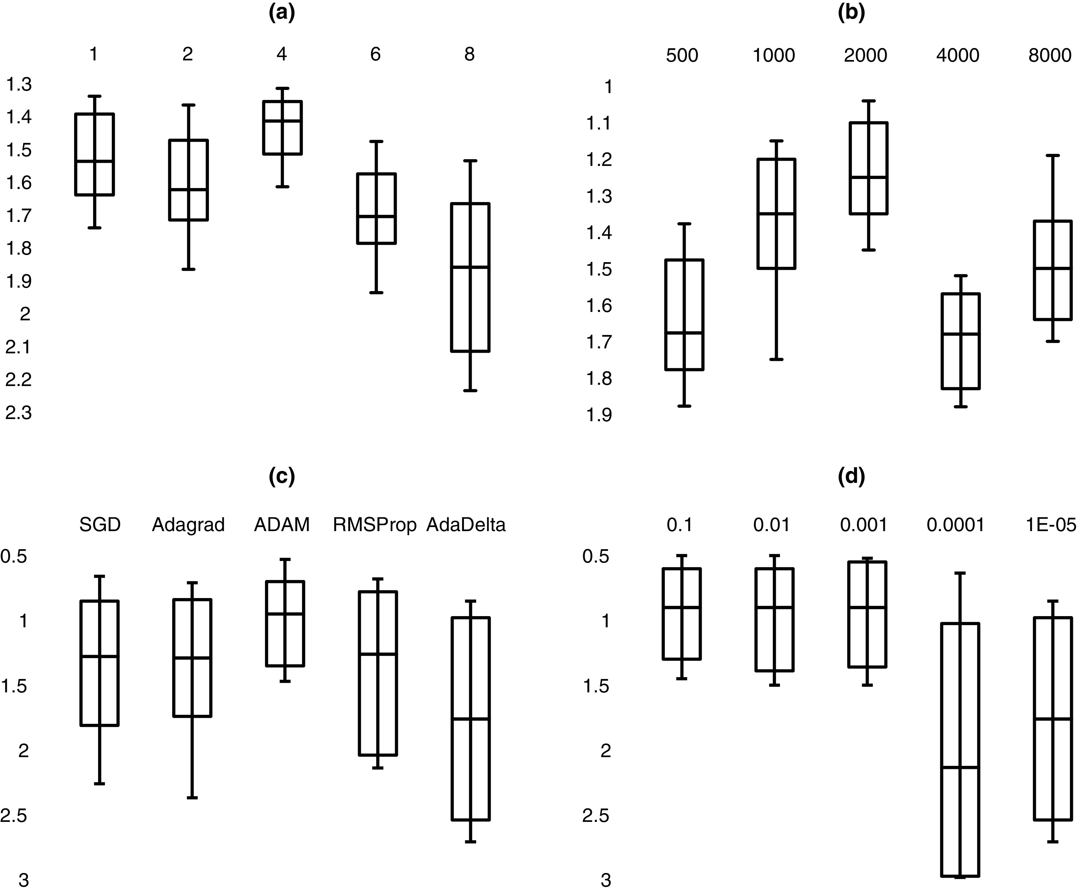
Figure 2: Box plots of hyper-parameters’ assessment based on nodes, epochs, choice and learning rate (a) No of nodes (b) No of epochs (c) Optimizer (d) Learning rate
The optimization algorithm was the third tuned hyper-parameter of the present LSTM model. Various optimization algorithms such as Stochastic Gradient Descent (SDG), Adagrad, Adam, AdaDelta, and RMSProp, were tested. The Adam (Adaptive Moment Estimation) algorithm is an extension of SGD that calculates each parameter's learning rate, such as alpha, beta1, beta2 and epsilon [52,53]. The experimental cases based on ten runs showed a better average RMSE value of 0.95 while using the ADAM optimizer's default parameters in Keras 2.3. AdaDelta showed an average RMSE value of 1.76 with high variance (Fig. 2C).
Learning rate (LR) was the fourth tuned parameter in the current study. The effects of different learning rates for the ADAM optimizer were evaluated; the default value of parameter LR in Keras is 0.001. Similarly, the default value for β1 is 0.9. In the same way, β2 is specified to be 0.999 and ε is specified to be 1e-07. An attempt was made to tune the learning rate with values of 0.1, 0.01, 0.001, 0.0001, and 0.00001. The box plot indicated that LR of 0.1, 0.01, and 0.001 showed good RMSE values of 0.9 and less variance without any significant difference. On the contrary, LR of 0.0001 and 0.00001 showed slightly lower RMSE values with higher variances (Fig. 2D). It was observed that the tuned LSTM model with four nodes, trained for 2000 epochs with ADAM optimizer having lr of 0.1, showed promising performance based on RMSE and computational efficiency in the current investigation.
An AutoRegression (AR) based model was used in the present investigation to compare the forecasting performance of the LSTM model (Fig. 3). Autoregression worked on the dataset without trend and seasonality, and therefore, the time series data preprocessed in Section 3.5 was utilized for autoregression. The AR package was used from the statsmodel library using Python to develop Model 3. The tuning of n, trend parameter, and the seasonal parameter was crucial to obtain the optimized forecasting model. The k values ranging from 1 to 24 months were given to model using a loop to obtain the optimized autoregression model. The optimized value for k was 12 steps or previous months value. The trend parameter and seasonal parameter were n and True, respectively. The average RMSE and R2 values for the autoregression model were 0.65 and 0.76, respectively for all the 5 basins, which was significantly good.
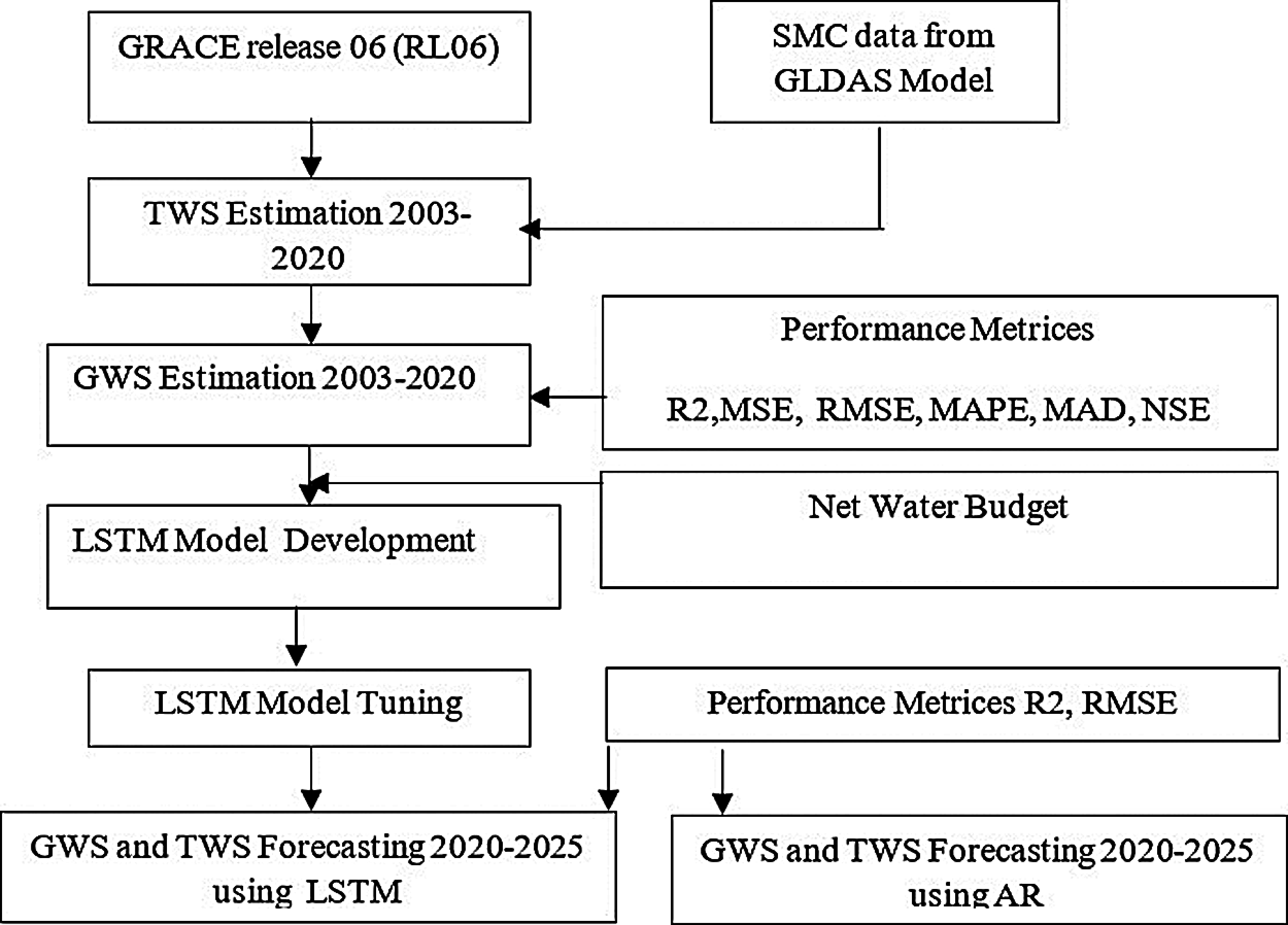
Figure 3: Flowchart of the methodology
3.9 Uncertainty Assessment of the LSTM Model
The Moment Correlation Coefficient (MCC), Root Mean Square Error (RMSE), Mean Absolute Percentage Error (MAPE) and Nash-Sutcliffe coefficient (NSE) were utilized to evaluate the uncertainty of the LSTM model output. The Mean Absolute Deviation (MAD) was also considered to analyze the LSTM model's accuracy between measured and predicted values.
The MCC summarizes the direction and degree of linear relations between actual and modeled datasets. The correlation coefficient can take values between −1 (perfectly negative correlation) through 0 (no correlation) to +1 (perfectly positive correlation). The MCC formula to compute the correlation coefficient is given in Eq. (14).
Here, N represents the number of pairs of data. The terms X and Y are parameters.
RMSE is a method to calculate the error or accuracy in predicting models based on standard deviation Eq. (15). The final output is given in a standard deviation of the error's magnitude, as per Eq. (15); the individual calculations are outputted as residuals based on [15].
Here, P_i is the ith LSTM predicted value, and Oi is the ith original value.
The MAPE method was used to calculate the prediction accuracy of the LSTM forecast. The calculation was based on the difference between the original values and values forecasted by the LSTM and dividing the original value difference. It was then multiplied by the number of observations and 100 to obtain the percentage error, Eq. (16) [19].
Here,
where Pi is the ith data value,
The NSE or efficiency coefficient test determines the magnitude between the variance of residual time series and variance of actual data, and its value ranges from -∞ to 1, see Eq. (18). An output near to one indicates higher model quality and reliability. A value below zero suggests that the model is not reliable. NSE test has been utilized in various GWS forecasting models [35,36,38,39].
where y,
4.1 Trend Analysis of GWSC, TWSC and Rainfall
As described earlier, the total uncertainty based on the first residual, second residual and the standard deviation of the second residual was computed for TWSC (±1.2 mm/year). The uncertainty in SMC based on the mean monthly standard deviation from the three GLDAS models was computed as ±0.2 (mm/year). Therefore, the total uncertainty for GWSC was 1.5 (mm/year). Results with a confidence factor ≥ of 90% indicate decreasing annual TWSC and GWSC change for all the five sub-basins (Tab. 1).

The analysis of rainfall data from 26 MET stations from 2009 to 2018 showed an interesting trend. Areas 1, 3 and 5 showed a slight increase in rainfall from 2009–2018; however, areas 2 and 4 showed no rainfall change for the same observation years. The rainfall period showed two peaks, one in winter [November-January] and another in summer [March-April]. A positive increasing trend of 0.2 mm/year was observed with a confidence factor ≥ of 80% when combined areas were taken into account. Based on METRain data, for Saudi Arabia, the average annual rainfall value increased from 52 mm for the year 2000 to 60 mm for the year 2015 [15] and 73.34 mm for the year 2018 in the present investigation. A positive trend in the long-term forecasted rainfall was also reported by [22,54].
4.2 Correlation Analysis Between SATRain, METRain, TWSC and GWSC
The MCC was performed to understand the relationship between GWSC, TWSC, SatRain and METRain for the five basins from January 2009 to December 2016 as per the common temporal dataset availability (Eq. (14)). There was a strong correlation between TWSC and GWSC; however, there was no correlation between TWSC and rainfall (SatRain and METRain) or GWSC and rainfall (SatRain and METRain). It is essential to mention that a significant association between the magnitudes of GWSC and rainfall cannot be expected. This is because the rainfall might be reallocated as surface runoff and evapotranspiration, thus altering the allocation of rainfall in terms of space and time and, consequently, the groundwater storage as the allocated volume [21,35]. The correlation coefficient between METRain and SatRain was significantly suitable for basin 1(0.72), basin 3(0.85) and basin 5(0.65); however, it was weak for basin 2(0.41) and basin 4(0.46).
4.3 Comparison with Other Studies
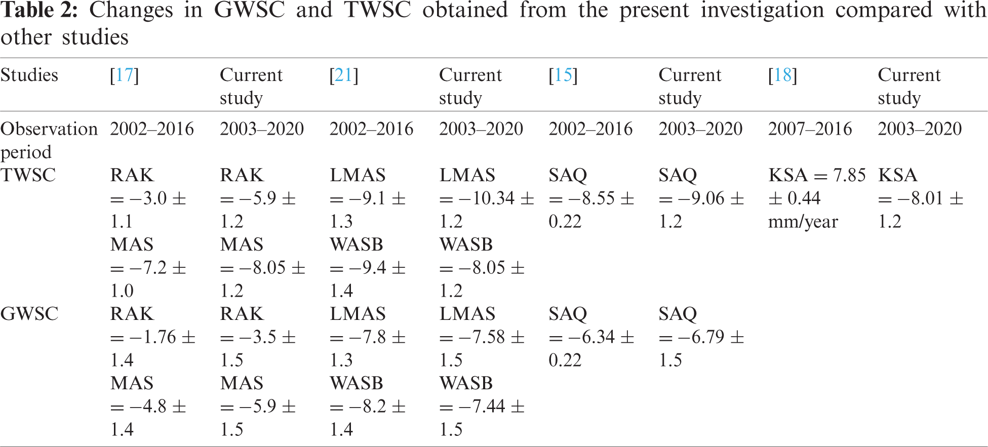
We have processed GRACE TWSC and GWSC for the KSA; therefore, we have compared the current investigation results with other studies (Tab. 2). It was evident based on comparison with other studies [15,17,18,21] that the TWSC and GWSC values observed in the present investigation were in suitable conformity with outcomes from other investigations regarding the scale of calculated uncertainties. The forecasting performance of the current study was compared with other benchmarks studies based on R2 and RMSE values [34–36,39–41] (Tab. 3). It was observed based on performance metrices that the present study showed better results.

4.4 LSTM-Based Forecasting of GWSC and TWSC from Jul 2020 – Dec 2025
There was a possibility while predicting the future values that the LSTM model output may be uncertain as the model's output was fed back into it as input. Therefore, we initially forecasted TWS and GWS from July 2015 to June 2020 and compared them with the actual values based on the values of coefficient of determination, RMSE, MSE, MAPE, and MAD (Tab. 4). The developed LSTM model was likely to accurately estimate the possible future values of GWS and TWS from July 2020 to Dec. 2025, given its reliability (Fig. 4).

The area of the basins with the respective volume of TWSC and GWSC from January 2003 to June 2020 (Tab. 5) shows that basin 1 has shown the maximum TWS volume withdrawn and GWS volume withdrawn at −5.387 (km3/year) and −3.206 (km3/year), respectively, from 2003 to 2020. While comparing the rate of historical (2003–2020) extracted groundwater (GWS) with the forecasted (2020–2025) rate of extracted groundwater (GWS), it was observed that basin three and basin one had shown higher rates −29.68% and −29.58%, while the other three basins had shown rates ranging from −8.89% to 13.66%.
In the absence of the data on groundwater wells in Saudi Arabia, the annual extracted groundwater dataset [55] was used to validate the GRACE-derived GWS for Saudi Arabia (2010–2016). The selection of this annual data for Saudi Arabia was justified by its distinctiveness and accessibility within the analysis duration. The correlation of GRACE GWS was performed with net extracted water based on MCC (see Eq. (14)). It was observed that the GWS GRACE estimations were significantly correlated (R = 0.87) with extracted groundwater data from [55], see Tab. 6.
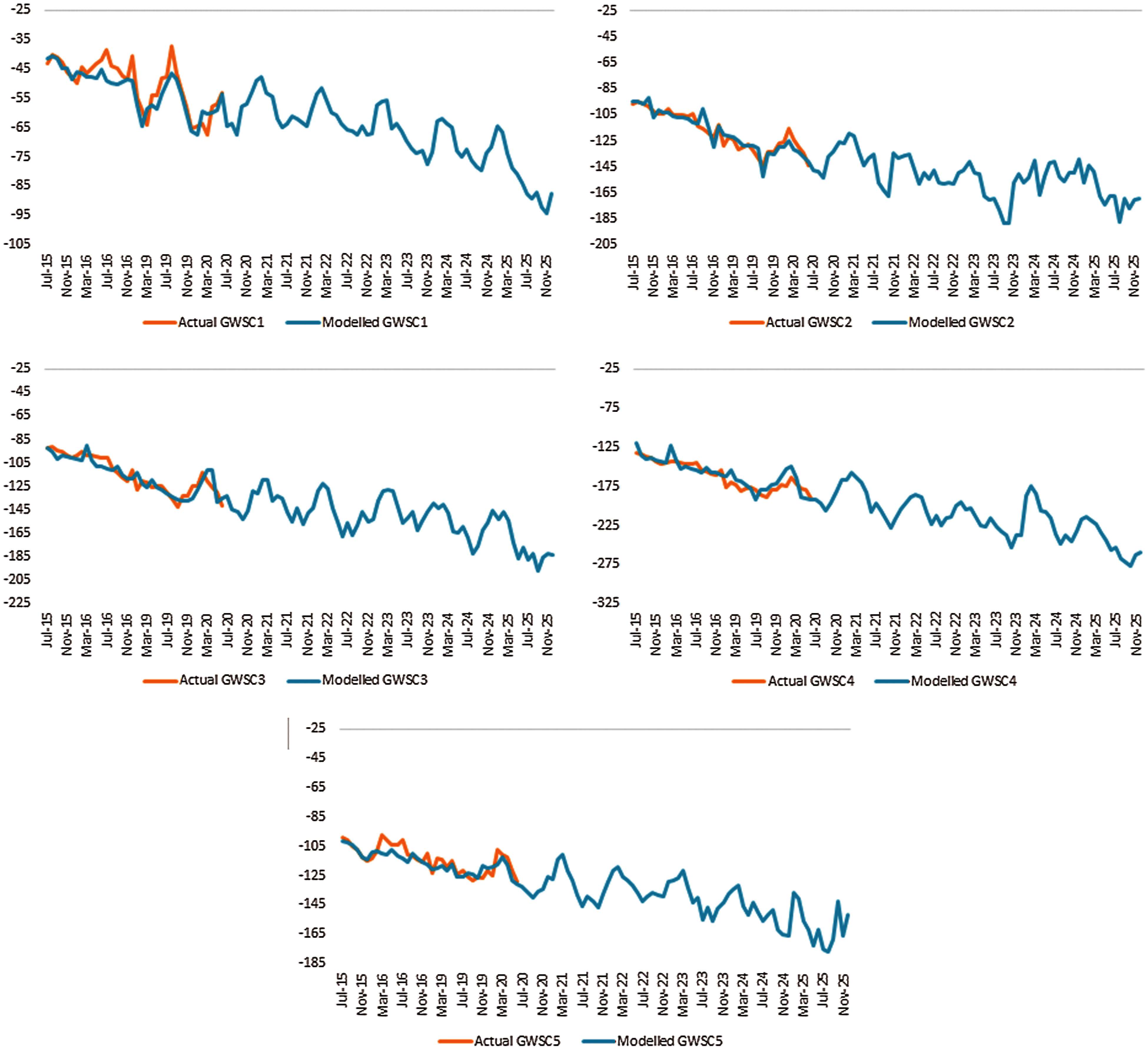
Figure 4: Comparison between actual monthly GWSC values (orange curve) and LSTM-forecasted GWSC values (blue curve)
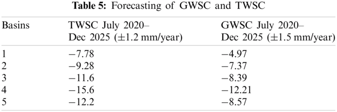

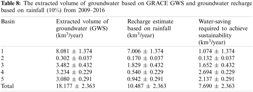
However, the present investigation found that the depletion rate did not show steady or increasing trends until June 2020. LSTM-based forecasting until 2025 also suggested that there is a requirement for sustainable water resources planning (Tab. 7). Another interesting observation was that when the volume of extracted groundwater based on GRACE GWS data of Jan-June (2019) was compared with GRACE GWS data of Jan-June (2020), a slight decrease of 0.5% was observed in groundwater extraction. In other words, groundwater extraction was lesser in 2020 than in 2019 (Tab. 8). It might be related to the slowdown or lockdown effect due to the COVID-19 pandemic.

4.5 Computational Efficiency of the Present Investigation
During the model tuning, there were clear differences between the number of iterations and associated computational time required. It was often found that the best suited LSTM model in the present investigation used 3 sec/epochs, whereas the LSTM model developed by [35] consumed 85 sec/epoch. The optimized model took only 25% computational time compared to the model with 8000 epochs in 400 min.
The present investigation provides an understanding of the historical and projected GWS changes at a large-scale using GRACE data for Saudi Arabia. Deep Learning LSTM models were developed based on rigorous hyper-parameters tuning to forecast the water storage changes based on GRACE-derived GWS. The major hyper-parameters of LSTM tuned in the present investigation were (1) number of nodes, (2) number of training epochs, (3) choice of optimizer, and (4) learning rate. A walk-forward model evaluation using the hyper-parameters mentioned above was attempted for different configuration values. The optimized model took 25% computational time compared to the model, which took 8000 epochs in 400 min. The correlation coefficient, MAPE, MAD, NSE and RMSE values were applied to test the LSTM models’ outcomes. GRACE-derived GWS indicated that all the five investigated basins were experiencing groundwater depletion rates of 18.17 km3/year. Future forecasting based on the developed LSTM model indicates that, from July 2020 to Dec 2025, the investigated five basins are likely to experience depletion of water at rates ranging from −7.78 ± 1.2 to −15.6 ± 1.2 for TWSC and −4.97 ± 1.5 to −12.21 ± 1.5 for GWS. The future scope of the present investigation is to add in-situ data when available to assess and improve the model performance.
6 Limitations and Learning Points of the Present Investigation
The significant limitations of the present study can be discussed with respect to the following points: (1) Data continuity and temporal availability of different datasets. GRACE data was available from 2002 to 2020 with data gaps in 2002 and 2017–2018 due to no data or no coverage. (2) Different resolutions of the dataset, e.g., GLDAS resolution was 1.0o, and GRACE-derived GWS and TWS were gridded to 1.0o. Similarly, SatRain resolutions were 0.25o and 0.10o for TRMM and GPM, respectively. (3) GWS and TWS were the change rate values, whereas SatRain and METRain were the time series data. (4) In the absence of data about groundwater wells for entire Saudi Arabia, the annual extracted groundwater dataset [1] were used to validate the GRACE-derived GWS for the study area, which was available only from 2010 to 2016. (5) The computation of the LSTM best fit model requires 100 min for 2000 number of epochs, and an improvement to use a lower number of epochs is required in the future so that model computational efficiency can become better. (6) The reasons to choose LSTM in the present investigation are its capability to deal with the vanishing gradient problem and better control, flexibility and performance than traditional RNN. (7) The LSTM model has limitations such as requirement of high memory-bandwidth due to linear layers, more prone to overfitting, and too complex to apply dropout.
Acknowledgement: We thank the anonymous referees for their useful suggestions.
Funding Statement: The authors extend their appreciation to the deputyship for Research & Innovation, Ministry of Education in Saudi Arabia, for funding this research work through the project number (IFP-2020–14).
Conflicts of Interest: The authors declare that they have no conflicts of interest to report regarding the present study.
1. Saudi General Authority for Statistics, “General authority for statistics,” https://stats.gov.sa/en/, 2018. [Google Scholar]
2. M. A. Haq, K. Jain, M. Shoab and K. P. R. Menon, “Estimation of terrestrial water storage change in the bhagirathi ganga and vishnu ganga basins using satellite gravimetry,” in Proc. IGARSS 2013, Melbourne, pp. 1817–1820, 2013. [Google Scholar]
3. L. Zheng, Y. Pan, H. Gong, Z. Huang and C. Zhang, “Comparing groundwater storage changes in two main grain producing areas in China: Implications for sustainable agriculturalwater resources management,” Remote Sensing, vol. 12, no. 13, pp. 1–21, 2020. [Google Scholar]
4. J. S. Famiglietti, M. Lo, S. L. Ho, J. Bethune, K. J. Anderson et al., “Satellites measure recent rates of groundwater depletion in california's central valley,” Geophysical Research Letters, vol. 38, no. 3, pp. 1–3, 2011. [Google Scholar]
5. J. Wahr, M. Molenaar and F. Bryan, “Time variability of the earth's gravity field: Hydrological and oceanic effects and their possible detection using GRACE,” Journal of Geophysical Research: Solid Earth, vol. 102, no. B12, pp. 30205–30229, 1998. [Google Scholar]
6. Z. M. Nigatu, D. Fan, W. You and A. M. Melesse, “Hydroclimatic extremes evaluation using grace/grace-fo and multidecadal climatic variables over the Nile river basin,” Remote Sensing, vol. 13, no. 4, pp. 651, 2021. [Google Scholar]
7. N. A. A. Gido, H. Amin, M. Bagherbandi and F. Nilfouroushan, “Satellite monitoring of mass changes and ground subsidence in sudan's oil fields using GRACE and sentinel-1 data,” Remote Sensing, vol. 12, no. 11, pp. 1–20, 2020. [Google Scholar]
8. M. Rodell, I. Velicogna and J. S. Famiglietti, “Satellite-based estimates of groundwater depletion in India,” Nature, vol. 460, no. 7258, pp. 999–1002, 2009. [Google Scholar]
9. D. Long, X. Scanlon, R. Bridget, Y. Wada, Y. Hong et al., “Have GRACE satellites overestimated groundwater depletion in the northwest India aquifer?,” Scientific Reports, vol. 6, no. 24398, pp. 1–38, 2016. [Google Scholar]
10. S. Srivastava and O. Dikshit, “Seasonal and trend analysis of TWS for the indo-gangetic plain using GRACE data,” Geocarto International, vol. 35, no. 12, pp. 1343–1359, 2020. [Google Scholar]
11. K. Tian, Z. Wang, F. Li, Y. Gao, Y. Xiao et al., “Drought events over the Amazon river basin (1993–2019) as detected by the climate-driven total water storage change,” Remote Sensing, vol. 13, no. 6, pp. 1–18, 2021. [Google Scholar]
12. M. Xiao, A. Koppa, Z. Mekonnen, B. R. Pagán, S. Zhan et al., “How much groundwater did california's central valley lose during the 2012–2016 drought?,” Geophysical Research Letters, vol. 44, no. 10, pp. 4872–4879, 2017. [Google Scholar]
13. X. Yang, S. Tian, W. Feng, J. Ran, W. You et al., “Spatio-temporal evaluation of water storage trends from hydrological models over Australia using GRACE mascon solutions,” Remote Sensing, vol. 12, no. 21, pp. 1–26, 2020. [Google Scholar]
14. E. C. Massoud, Z. Liu, A. Shaban and M. El Hage, “Groundwater depletion signals in the beqaa plain, Lebanon: Evidence from GRACE and sentinel-1 data,” Remote Sensing, vol. 13, no. 5, pp. 1–15, 2021. [Google Scholar]
15. O. A. Fallatah, M. Ahmed, D. Cardace, T. Boving and A. S. Akanda, “Assessment of modern recharge to arid region aquifers using an integrated geophysical, geochemical, and remote sensing approach,” Journal of Hydrology, vol. 569, no. October, pp. 600–611, 2019. [Google Scholar]
16. O. A. Fallatah, M. Ahmed, H. Save and A. S. Akanda, “Quantifying temporal variations in water resources of a vulnerable middle Eastern transboundary aquifer system,” Hydrological Processes, vol. 31, no. 23, pp. 4081–4091, 2017. [Google Scholar]
17. M. Sultan, N. C. Sturchio, S. Alsefry, M. K. Emil, M. Ahmed et al., “Assessment of age, origin, and sustainability of fossil aquifers: A geochemical and remote sensing-based approach,” Journal of Hydrology, vol. 576, no. May, pp. 325–341, 2019. [Google Scholar]
18. A. Pradipta, M. H. Makkawi, H. Sharif, A. Elamin and S. Kaka, “The sustainability of Saudi Arabia’s water resources from the past decade: A remote sensing approach,” King Fahd University of Petroleum & Minerals, vol. 1, pp. 1–10, 2018. [Google Scholar]
19. A. Qian, S. Yi, L. Chang, G. Sun and X. Liu, “Using GRACE data to study the impact of snow and rainfall on terrestrial water storage in northeast China,” Remote Sensing, vol. 12, no. 24, pp. 1–21, 2020. [Google Scholar]
20. M. Liu, L. Min, Y. Shen and L. Wu, “Evaluating the impact of alternative cropping systems on groundwater consumption and nitrate leaching in the piedmont area of the north China plain,” Agronomy, vol. 10, no. 11, pp. 1–20, 2020. [Google Scholar]
21. A. Othman, M. Sultan, R. Becker, A. Alsefry, T. Alharbi et al., “Use of geophysical and remote sensing data for dssessment of aquifer depletion and related land deformation,” Surveys in Geophysics, vol. 39, no. 3, pp. 543–566, 2018. [Google Scholar]
22. Y. Wehbe and M. Temimi, “A remote sensing-based assessment of water resources in the Arabian Peninsula,” Remote Sensing, vol. 13, no. 2, pp. 1–17, 2021. [Google Scholar]
23. J. Zhao, D. Zeng, S. Liang, H. Kang and Q. Liu, “Prediction model for stock price trend based on recurrent neural network,” Journal of Ambient Intelligence and Humanized Computing, vol. 12, no. 1, pp. 745–753, 2021. [Google Scholar]
24. K. Greff, R. K. Srivastava, J. Koutnik, B. R. Steunebrink and J. Schmidhuber, “LSTM: A search space odyssey,” IEEE Transactions on Neural Networks and Learning Systems, vol. 28, no. 10, pp. 2222–2232, 2017. [Google Scholar]
25. X. Liu, Y. Si and D. Wang, “Lstm neural network for beat classification in ECG identity recognition,” Intelligent Automation & Soft Computing, vol. 26, no. 2, pp. 341–351, 2020. [Google Scholar]
26. A. Jabeen, S. Afzal, M. Maqsood, I. Mehmood, S. Yasmin et al., “An lstm based forecasting for major stock sectors using covid sentiment,” Computers, Materials & Continua, vol. 67, no. 1, pp. 1191–1206, 2021. [Google Scholar]
27. C. Hu, Q. Wu, H. Li, S. Jian, N. Li et al., “Deep learning with a long short-term memory networks approach for rainfall-runoff simulation,” mdpi Water, vol. 10, no. 11, pp. 15–43, 2018. [Google Scholar]
28. K. Fang and C. Shen, “Near-real-time forecast of satellite-based soil moisture using long short-term memory with an adaptive data integration kernel,” Journal of Hydrometeorology, vol. 21, no. 3, pp. 399–413, 2020. [Google Scholar]
29. M. -J. Shin, S. -H. Moon, K. G. Kang, D. -C. Moon and H. -J. Koh, “Analysis of groundwater level variations caused by the changes in groundwater withdrawals using long short-term memory network,” Hydrology, vol. 7, no. 3, pp. 1–15, 2020. [Google Scholar]
30. B. D. Bowes, J. M. Sadler, M. M. Morsy, M. Behl and J. L. Goodall, “Forecasting groundwater table in a flood prone coastal city with long short-term memory and recurrent neural networks,” Water, vol. 11, no. 1098, pp. 1–38, 2019. [Google Scholar]
31. J. Zhang, Y. Zhu, X. Zhang, M. Ye and J. Yang, “Developing a long short-term memory (LSTM) based model for predicting water table depth in agricultural areas,” Journal of Hydrology, vol. 561, pp. 918–929, 2018. [Google Scholar]
32. F. Wang, Y. Chen, Z. Li, G. Fang, Y. Li et al., “Developing a long short-term memory (LSTM)-based model for reconstructing terrestrial water storage variations from 1982 to 2016 in the Tarim river basin, northwest China,” Remote Sensing, vol. 13, no. 5, pp. 1–18, 2021. [Google Scholar]
33. M. Ahmed, M. Sultan, T. Elbayoumi and P. Tissot, “Forecasting GRACE data over the african watersheds using artificial neural networks,” Remote Sensing, vol. 11, no. 15, pp. 1–21, 2019. [Google Scholar]
34. P. Malakar, A. Mukherjee, S. N. Bhanja, S. Sarkar, D. Saha and R. K. Ray, “Deep learning-based forecasting of groundwater level trends in India: Implications for crop production and drinking water supply,” ACS ES&T Engineering, vol. 1, no. 6, pp. 965–977, 2021. [Google Scholar]
35. A. Wunsch, T. Liesch and S. Broda, “Groundwater level forecasting with artificial neural networks: A comparison of LSTM, CNN and NARX,” Hydrological Earth System and Science Discussion, vol. 552, no. November, pp. 1–23, 2020. [Google Scholar]
36. A. T. M. S. Rahman, T. Hosono, J. M. Quilty, J. Das and A. Basak, “Multiscale groundwater level forecasting: Coupling new machine learning approaches with wavelet transforms,” Advances in Water Resources, vol. 141, no. April, pp. 1–14, 2020. [Google Scholar]
37. D. S. K. K. V. R. Satya Sai and A. Manjunath, “Groundwater level forecasting using gravity recovery and climate experiment (GRACE) by artificial neural network (ANN) for Krishna river sub-basin,” Solid State Technologu, vol. 63, no. 2, pp. 2300–2316, 2020. [Google Scholar]
38. M. Moravej, P. Amani and S. M. Hosseini-Moghari, “Groundwater level simulation and forecasting using interior search algorithm-least square support vector regression (ISA-LSSVR),” Groundwater Sustainability Development, vol. 11, no. May, pp. 100447, 2020. [Google Scholar]
39. T. Guo, S. Song, J. Shi and J. Li, “Groundwater depth forecasting using configurational entropy spectral analyses with the optimal input,” Groundwater, vol. 58, no. 5, pp. 749–758, 2020. [Google Scholar]
40. A. Getirana, M. Rodell, S. Kumar, H. K. Beaudoing, K. Arsenault et al., “GRACE improves seasonal groundwater forecast initialization over the United States,” Journal of Hydrometeorology, vol. 21, no. 1, pp. 59–71, 2020. [Google Scholar]
41. Z. S. Ahmadi, H. R. Safavi and M. Zekri, “Forecasting groundwater level under climate change and water resources management scenarios,” Journal of Water and Wastewater, vol. 31, no. 6, pp. 1–15, 2021. [Google Scholar]
42. S. N. Bhanja and A. Mukherjee, “In situ and satellite-based estimates of usable groundwater storage across India: Implications for drinking water supply and food security,” Advances in Water Resources, vol. 126, pp. 15–23, 2019. [Google Scholar]
43. M. M. Watkins, D. N. Wiese, D. N. Yuan, C. Boening and F. W. Landerer, “Improved methods for observing earth's time variable mass distribution with GRACE using spherical cap mascons,” Journal of Geophysical Research: Solid Earth, vol. 120, no.4, pp. 2648–2671, 2015. [Google Scholar]
44. M. Rodell P. R. Houser, U. Jambor, J. Gottschalck, K. Mitchell et al., “The global land data assimilation system,” Bulletin of the American Meteorological Society, vol. 85, no. 3, pp. 381–394, 2004. [Google Scholar]
45. H. L. Rui and H. Beaudoing, “Readme document for nasa gldas version 2 data products,” Goddard Earth Sciences Data and Information Services Center, vol. 2, pp. 1–22, 2020. [Google Scholar]
46. E. P. Maurer, A. W. Wood, J. C. Adam, D. P. Lettenmaier and B. Nijssen, “A long-term hydrologically based dataset of land surface fluxes and states for the conterminous United States,” Journal of Climate, vol. 15, no. 22, pp. 3237–3251, 2002. [Google Scholar]
47. B. R. Scanlon, Z. Zhang, H. Save, D. N. Wiese, F. W. Landerer et al., “Global evaluation of new GRACE mascon products for hydrologic applications,” Water Resources Research, vol. 52, no. 12, pp. 9412–9429, 2016. [Google Scholar]
48. H. B. Mann, “Nonparametric tests against trend,” Econometrica, vol. 13, pp. 245–259, 1945. [Google Scholar]
49. M. Kendall, Rank correlation methods, Griffin, London, 1970. [Google Scholar]
50. P. K. Sen, “Estimates of the regression coefficient based on kendall's Tau,” Journal of the American Statistical Association, vol. 63, no. 324, pp. 1379–1389, 1968. [Google Scholar]
51. R. Schumacker, S. Tomek, R. Schumacker and S. Tomek, “z-Test,” in Understanding Statistics Using R, Newyork: Springer, 2013. [Google Scholar]
52. J. Duchi, E. Hazan and Y. Singer, “Adaptive subgradient methods for online learning and stochastic optimization,” in Proc. COLT 2010, Berkeley, pp. 257–269, 2010. [Google Scholar]
53. D. P. Kingma and J. Ba, “Adam: A method for stochastic optimization,” in Proc. ICLR 2015, San Diego, pp. 1–15, 2014. [Google Scholar]
54. S. Chowdhury and M. Al-Zahrani, “Characterizing water resources and trends of sector wise water consumptions in Saudi Arabia,” Journal of King Saud University - Engineering Sciences, vol. 27, no. 1, pp. 68–82, 2015. [Google Scholar]
55. GAS, “Population estimates general authority for statistics,” General Authority for Statistics Kingdom of Saudi Arabia, 2021, Accessed Apr. 08, 2021. https://www.stats.gov.sa/en/43. [Google Scholar]
 | This work is licensed under a Creative Commons Attribution 4.0 International License, which permits unrestricted use, distribution, and reproduction in any medium, provided the original work is properly cited. |