Computers, Materials & Continua DOI:10.32604/cmc.2022.020483
Article

Novel Quantum Algorithms to Minimize Switching Functions Based on Graph Partitions

Peng Gao*, Marek Perkowski, Yiwei Li and Xiaoyu Song

Department of Electrical and Computer Engineering, Portland State University, Portland, Oregon, 97201, USA
*Corresponding Author: Peng Gao. Email: Pengao@pdx.edu
Received: 26 May 2021; Accepted: 20 July 2021

Abstract: After Google reported its realization of quantum supremacy, Solving the classical problems with quantum computing is becoming a valuable research topic. Switching function minimization is an important problem in Electronic Design Automation (EDA) and logic synthesis, most of the solutions are based on heuristic algorithms with a classical computer, it is a good practice to solve this problem with a quantum processer. In this paper, we introduce a new hybrid classic quantum algorithm using Grover’s algorithm and symmetric functions to minimize small Disjoint Sum of Product (DSOP) and Sum of Product (SOP) for Boolean switching functions. Our method is based on graph partitions for arbitrary graphs to regular graphs, which can be solved by a Grover-based quantum searching algorithm we proposed. The Oracle for this quantum algorithm is built from Boolean symmetric functions and implemented with Lattice diagrams. It is shown analytically and verified by simulations on a quantum simulator that our methods can find all solutions to these problems.

Keywords: Boolean symmetric function; lattice diagrams; Grover’s searching algorithm

1  Introduction

Grover’s Algorithm [1] is one of few most famous and most useful quantum algorithms to which many decision and optimization problems can be reduced. And Grover’s algorithm can provide quadratic speedup comparing to its classical counterpart [1]. Problems in Graph Theory are excellent candidates to be solved using Grover’s Algorithm. We present a uniform approach to use Grover’s Algorithm for solving several problems in Graph Theory which has multiple applications such as minimization of binary circuits [2].

Hypercube graphs [3] are an important category of graphs in Graph Theory because they have many interesting properties, such as bipartiteness, Hamiltonicity, and symmetry. These properties make hypercubes useful to solve problems in network topology [4], parallel computing [5], multi-valued logic encoders/decoders [6], circuit switching modeling [7], and others.

Standard hypercubes are representations that are isomorphic to Karnaugh maps used in logic synthesis. Prime implicants of Boolean functions with n variables are sub-hypercubes or cliques with 2k nodes, k = 1,…, n. Hypercubes are generated by Cartesian products of binary vectors. Bettayeb introduced k-ary hypercubes [8] for computer networks. Here we introduce hybrid mixed hypercubes that are Cartesian products of arbitrary radix multi-valued vectors. We name them generalized hypercubes. The generalized hypercube inherits all properties of hypercube but with a more general structure corresponding to switching functions with mixed variables. These are isomorphic to Marquand charts [9] known from minimization of multi-valued switching circuits and Machine Learning.

Disjoint Sum of Products (DSOP) is one of commonly used form to minimize Boolean switching function. A DSOP realization of a Boolean function can be represented as a hypercube graph in which a realization with disjoint products of literals corresponds to disjoint partitioning to sub-hypercubes. This can be extended to Sum of Products (SOP) [10,11]. Unfortunately large size NP-hard problems must be solved to find the exact solution. Often the methods require also to generate astronomic numbers of prime or product implicants.

Solving these problems with classical computers, even parallel computers, seems to not lead to interesting results and even not much has been published in recent years on these topics. However, future quantum computers give a promise. With the fast development of quantum circuits, several researchers focus on creating quantum algorithms for problems in Graph Theory [12]. Although now only small problems can be solved, future quantum computers will be able to achieve “quantum supremacy.” This gives promise to the work presented here that is not practical at the moment [13].

Our paper proposes new quantum algorithms to find disjoint partitions of arbitrary graphs to E-regular graphs. E-regular graph is a regular graph in which all vertices have the same degree [14,15]. These algorithms are based on Grover’s searching algorithm and use efficient ways to build Grover Oracle with Boolean symmetric functions. A hybrid algorithm is composed of a quantum algorithm and a standard algorithm. The classical part of the algorithm is executed on the classical computer which prepares data and controls for the quantum computer and receives partial results from it. With such a hybrid algorithm, we are able to distinguish special cases of E-regular graphs such as cycles, standard hypercubes and some generalized hypercubes. (Cycles are graphs in which every node has exactly two neighbor nodes. E-regular graph is composed of one or more cycles).

Two types of problems can be formulated for E-regular graph partition.

Problem 1. Full graph partitioning. Find all disjoint partitions of an arbitrary graph to E-regular subgraphs for given E, such that every node of the graph belongs to one of these regular subgraphs.

Problem 2. Partial graph partitioning. Find all disjoint partitions of an arbitrary graph to E-Regular graphs for given E, such that every node belongs to one of these regular subgraphs or does not belong to any subgraph. We call this the partial partitioning.

Our hybrid quantum/classical algorithm in to solve the second type of problems can be applied to various some problems in minimizing switch circuit. The main innovative idea of our paper is to represent Graph Theory problems as collections of symmetric functions in which variables correspond to edges of the graph and nodes to certain constraints on them. Symmetric functions can be realized efficiently in multi-level circuits called lattices. Although our small examples below use for simplicity DSOP realizations of symmetric functions, it is important that for large functions the presented oracles should use optimized lattices [16].

The principle of the proposed methodology is to find some subsets of edges that satisfy various types of constraints related to symmetry. Many problems can be formulated as clustering, partitioning or covering with applications in logic synthesis and Machine Learning. Although we refer for details to our previous works [16,17], this paper is self-contained and has a sufficient amount of information to follow main principles of our approach.

This paper is organized as follows. Section 2 presents Boolean Symmetric functions and their efficient realization in quantum circuits for Grover oracles. In Section 3 we present two quantum algorithms based on Grover. Section 4 only briefly outlines Grover’s Algorithm that is well-known. those in which every node has at least one adjacent edge. Two problems are solved for E-regular graphs. Section 5 covers problems in Boolean Minimization.

2  Grover’s Algorithm

Grover’s algorithm is another function block in our hybrid algorithm. It is a quantum searching algorithm invented by Grover in 1996, In our algorithm the constraints are formulated with symmetric function blocks and the Grover’s algorithm is used as a solver to find the solutions for different problems. For problems with single solution Grover’s algorithm finds an input variable vector with high probability to satisfy the black-box Boolean function of the oracle, Fig. 1 is a diagram to present mainly function blocks of Grover’s searching algorithm. For problems with many solutions after finding the first solution, the oracle is modified by excluding this particular minterm (see explanation and example in [18]) and the Grover’s algorithm is run again. This is repeated until all solutions are found. A standard method used in applications in Grover’s algorithm where we want to find all solutions is to modify the oracle by exoring it with the products corresponding to the sets of solutions found. This reduces the space of remaining solutions (true minterms). This step is repeated until all found solutions are removed from the oracle. Details and oracle construction can be found in [19].

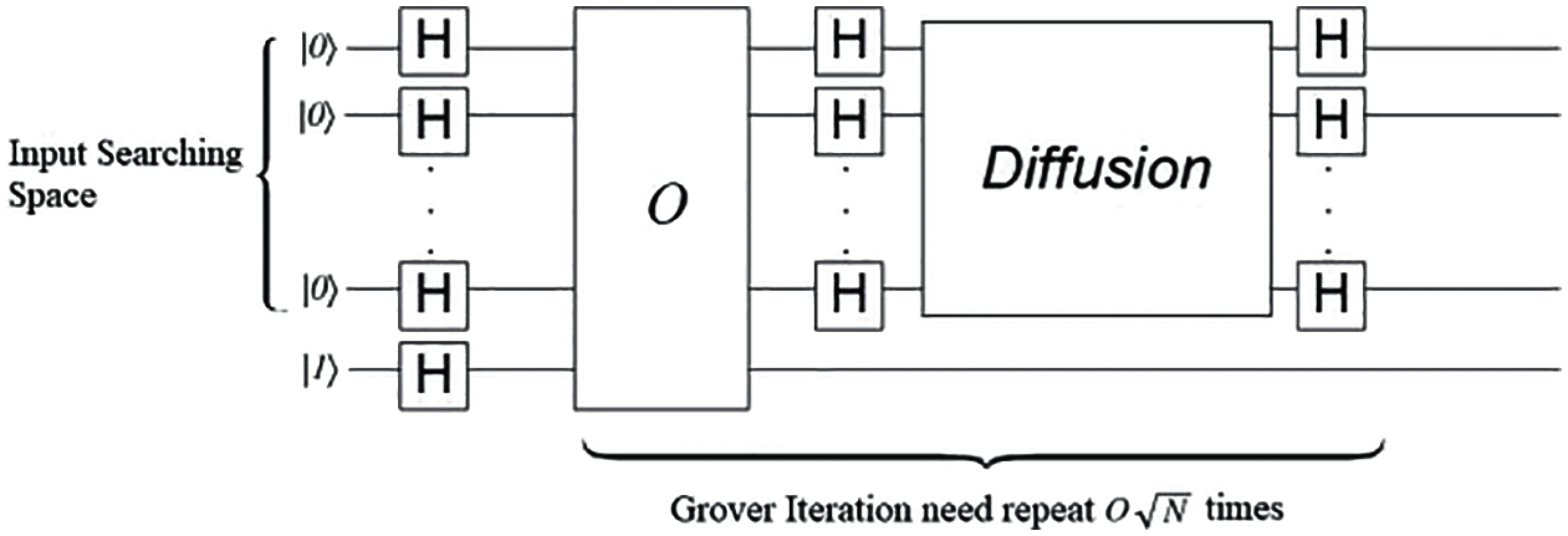
Figure 1: Grover’s algorithm

The input searching space of Grover’s algorithm is created by n-qubits quantum registers with Hadamard gate, then those input data will pass to oracle function, at this stage, oracle will inverse the phase of solution item, next step is called amplitude amplification, the diffusion operator will increase the amplitude (probability) of target item, and decrease others. After 2n iterations the amplitude of target item will be the highest probability item in a single measurement.

Oracle function in Grover’s algorithm should identify the target from input searching space, so it is problem-specific. There are many papers about Grover’s algorithm, but most of them do not pay attention to circuit complexity [20] and quantum cost [21] of oracles. Our approach can be characterized by an attempt to decrease the quantum cost of the oracle’s circuit. This paper follows the “engineering approach” to building quantum oracles where we create the oracle bottom up from simple blocks, possibly using ancilia qubits. This in contrast to several other authors that describe the oracle by a unitary matrix. Although their approach does not involve ancilia qubits it may lead to elementary gates that are not standard Toffoli, Feynman and NOT but arbitrary single qubit rotations and control rotations, which are very difficult or even impossible to realize in several practical existing quantum realization technologies.

3  Boolean Symmetric Functions and Lattice Diagrams for Oracles

In this section, the Boolean symmetric functions, Lattice diagrams are presented, the quantum layout of Lattice diagrams is shown in the end, this is the core part of symmetric blocks in our oracle.

Let f be a total Boolean function Bn → B, where B = {0, 1} and n > 1.

Definition 1. (Totally Symmetric Boolean Function) A Boolean function f is totally symmetric if its output is invariant under any permutation σ of its input bits:

Single index Symmetric Function S can be denoted as Sk, such that for every true minterm mi of S, the number of positive literals in all true minterms of this function is k, and the number of negative literals is n − k. For example a symmetric Boolean function F=a¯bc+ab¯c+abc¯ is denoted as S2. By a¯ we denote the negative literal. Each minterm of F: a¯bc,ab¯c,and abc¯ contains two positive literals. The n-variable Boolean function contains n + 1 symmetric index functions, from S0 to Sn. These symmetric indices can be combined as a multiple index symmetric functions, for instance S1 + S3 = S1 ⊕ S3 = S1,3.

3.1 Lattice Diagrams

There exist several classical structures to realize Boolean symmetric functions [22]. The idea of Lattice Diagram [23] originates from Universal Akers Arrays (UAA) [24], which are well known for their area-efficiency and planar layout. Lattice Diagrams inherit this property from UAA but in several cases are even more efficient. First, comparing to UAA’s rectangular shape, Lattice Diagrams start from a tree expansion, then combining non-isomorphic nodes at the same level, thus making the shape of Lattice Diagram to be a triangle or trapezoid shape, and only keeping the minimum necessary size of repeated variables. Secondly, instead of assuming only Shannon expansions in UAA, Lattice Diagrams can use not only Shannon expansions but also positive and/or negative Davio expansions [25]. As we know quantum reversible circuits are based on EXOR rather OR operators, therefore EXOR-based gates like Toffoli and Feynman are used [26,27], however, our paper is interested in those areas. This fact is important in quantum circuit synthesis, since Davio expansion can be mapped into Toffoli gate directly, which means Davio expansions lead to more efficient circuits than Shannon expansions which need two Toffoli gates. Lastly, Lattice Diagrams can handle multi-output functions, by changing the connection of nodes. This property makes Lattice diagram more powerful in synthesizing sets of symmetric functions. They are the base of our efficient oracles for large regular graphs. Their regularity and symmetry are good for 1-dimensional or 2-dimensional quantum layout [28], an issue very important from a practical realization point of view [29] of all types of circuit realization, but especially for quantum computing with respect to decoherence.

Fig. 2a in which signals flow from bottom to top presents a single output Lattice Diagram for function f(a, b, c); at the bottom there are small squares that can be filled with constants 0 or 1. For single output Lattice with n levels, we can realize every symmetric functions of n variables only by changing constants at the bottom level. Several functions of more than n variables and non-symmetric function of n variables can be realized with n-level Lattice. Fig. 2a is an example of 3-level Lattice with a single output, the bottom level nodes correspond to constants and simple Boolean functions such as a,a¯,a+b. Fig. 2b presents a multi-output Lattice diagram with the same size of variables as Fig. 2a, but the signal flow is reversed. It has similar structure as single output Lattice, only the direction of each node is opposite. That makes this generic Lattice to contain more constants than the single output Lattice. But that will not affect the size of circuit, since after circuit synthesis those constants can be removed and the circuit simplified using the well-known Boolean simplification method of “propagation of constants through the circuit”.

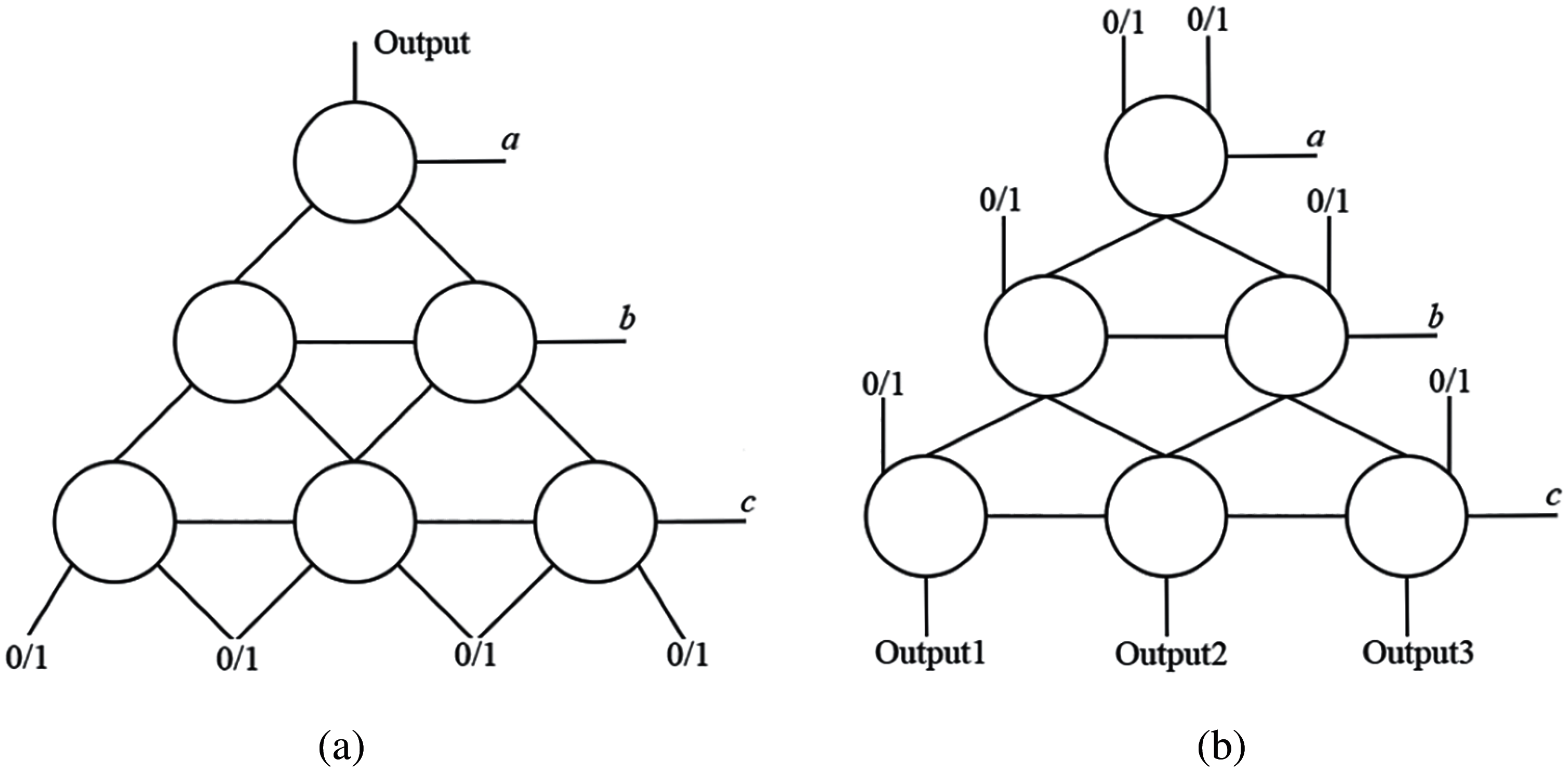
Figure 2: (a) Single output lattice diagram. (b) Multi-output lattice diagram

3.2 Using Lattice Diagrams to Implement Symmetric Boolean Functions

3.2.1 Mapping Symmetric Functions to Davio Lattices

As we mentioned, Lattice Diagrams can use either Shannon or Davio expansions. If every cell in a Lattice Diagram has a uniform expansion, then we name that Lattice by the expansion. Thus Shannon Lattice has all cells being Shannon expansions. Expansion type is an important characterization of Lattice Diagram, there are three types of expansions: Shannon, Positive Davio, and Negative Davio.

Let f0 and f1 be the positive and negative cofactors of a Boolean function f in respect to variable x1. Here f0 is f(0,x2,...,xn) with x1 replaced by 0, f1 is f(1,x2,...,xn) with x1 replaced by 1, f2=f0⊕f1 where symbol ⊕ means Exclusive-OR. We call f2 = f0 ⊕ f1 the Boolean difference of f for x1. Shannon expansion with respect to variable x1 is:

f(x1,x2,…,xn)=x1¯⋅f(0,x2,…,xn)⊕x1⋅f(1,x2,…,xn) (1)

Positive Davio expansion [1,5] with respect to variable x1 is:

f(x1,x2,…,xn)=f(0,x2,…,xn)⊕(x1⋅f(0,x2,…,xn)⊕f(1,x2,…,xn))=f0⊕x1f2 (2)

Negative Davio with respect to variable x1 is: f(x1,x2,...,xn)=f1⊕x¯1f2. Here we map the expansions to quantum Toffoli gates. It has been proved that Positive Davio Lattice (PDL) can be mapped into a quantum circuit with less quantum cost and smaller distance in Linear Nearest Neighbor (LNN) model. Comparing with Shannon Lattice, PDL is more efficient and inexpensive to implement into quantum circuit, that is why we choose it in our paper. For negative Davio Lattice, it can be easily transformed from PDL, so we will not discuss it separately. For positive Davio Lattice, each cell’s function is f(S,a,b)=a⊕(S⋅b) and its symbol is Fig. 3a. By changing the polarity of s, this cell can be used in negative Davio Lattice as well.

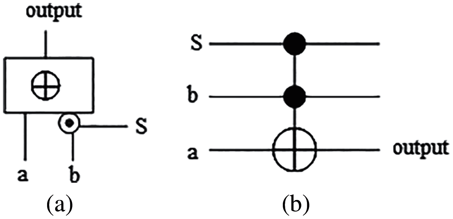
Figure 3: (a) Davio gate diagram, (b) Implementation of Davio gate with quantum Toffoli gate

Fig. 4 is a single-output positive Davio Lattice.

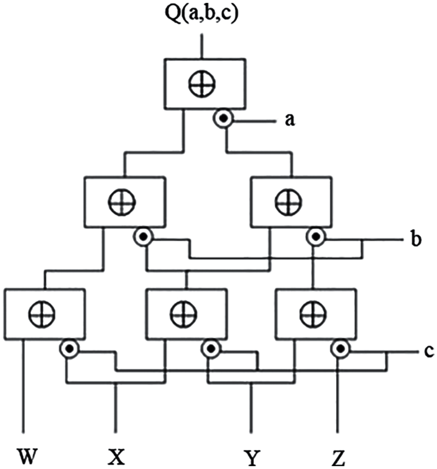
Figure 4: Single-output Davio lattice structure

The constants of the single-output lattice can be changed for different symmetric functions, more details and examples about constants and symmetric functions will be discussed in the next example. For multi-output lattices, the constants are determined by a specific symmetric function. This lattice has the capability to generate all symmetric functions by adding simple functions such as OR or EXOR on outputs. Given a Boolean function Q (a, b, c), it can be implemented by PDL layout from Fig. 4. The expansion function of each cell is a positive Davio gate. In this three-level positive Davio lattice, output equation is:

Q(a,b,c)=W⊕X⋅(a⊕b⊕c)⊕Y⋅(ab⊕bc⊕ac)⊕Z⋅(abc) (3)

We can find in this equation that every constant W, X, Y, Z is multiplied by a term that is a symmetric function. For example, a ⊕ b ⊕ c contains minterms: abc¯,ab¯c,a¯bc,abc, which is S1,3 (a, b, c). By selecting different coefficient values, the required symmetric function will be achieved at the output of this lattice. The sequence of coefficient constants W, X, Y, Z at the bottom of lattice is called a symmetry vector. Davio expansion is using Zhegalkin Normal Form (ZNF) [30], its polynomial expansion can be derived by a binary matrix called Zhegalkin Polynomial Matrix in Fig. 5. This matrix is generated with the following recursion: D0 = 1, Dj=[Dj−1Dj−10Dj−1], where j = 1, 2,…, m. Fig. 5 is the matrix used in our example.

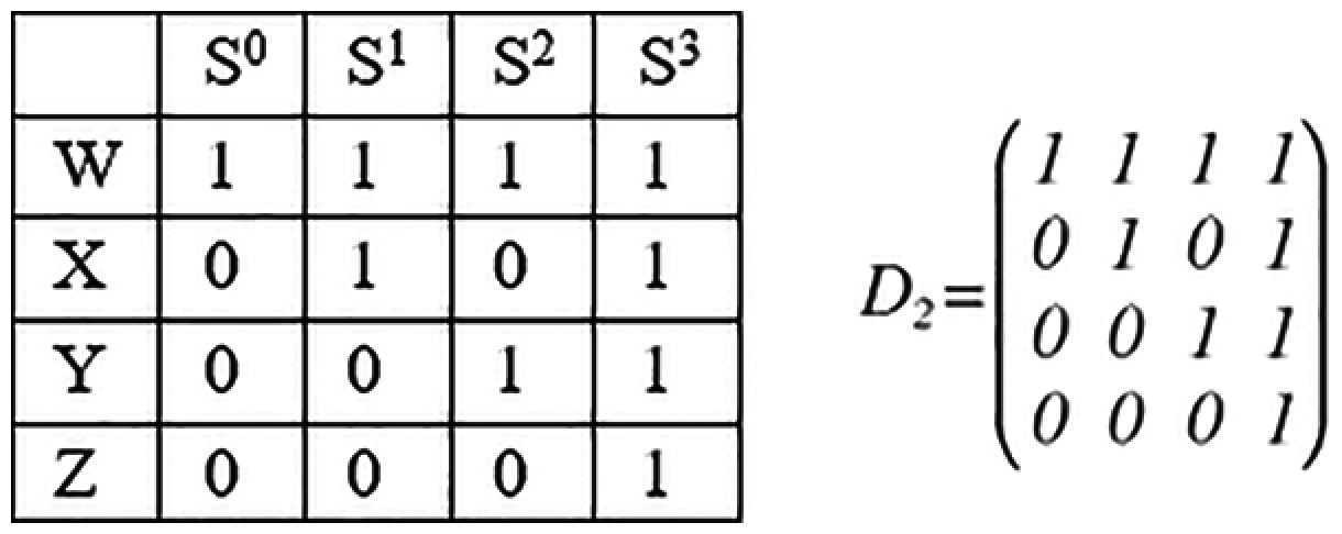
Figure 5: Zhegalkin polynomial matrix for 3 variables

In this matrix every row represents the “Davio cofactors” in Davio Lattice, every column represents symmetric functions from S0 to S3. For example, the row [0 1 0 1] means the related symmetric function of cofactor X is S1,3. Here we define the concept of Davio cofactor by analogy of the well-known concept of Shannon cofactor. The equation of Q (a, b, c) in Fig. 4 is expressed with symmetric functions:

Q(a,b,c)=W⋅S0,1,2,3⊕X⋅S1,3⊕Y⋅S2,3⊕Z⋅S3 (4)

In Davio Lattice, each cofactor is associated with a group of symmetric indices, by selecting different order of cofactors we can get all symmetric function indices. For example, if we need function S1, we can set X and Z to 1, and remaining cofactors to 0. In Davio Lattice all terms are connected with XOR gate, so the equation Q (a, b, c) becomes 0 ⊕ S1,3⊕ S3 ⊕0 = S1. Symmetric functions with related binary vectors [W, X, Y, Z] are the following: S0 = [1, 1, 1, 1] , S1 = [0, 1, 0, 1] , S2 = [0, 0, 1, 1] , S3 = [0, 0, 0, 1].

3.2.2 Mapping Davio Lattice into Quantum Reversible Circuit

Davio gate can be naturally mapped into a 3-inputs Toffoli gate, as shown in Fig. 3b. Davio Lattice can be directly mapped into a quantum circuit. Fig. 6a shows a positive Davio Lattice of symmetric function S2(a, b, c). Since the symmetry vector contains only constants, this circuit can be simplified by constants propagation, as in Fig. 6b. More details in [16].

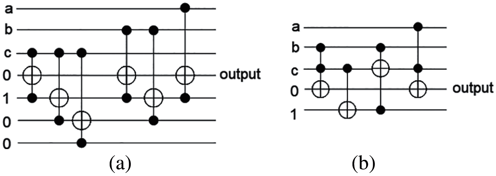
Figure 6: (a) Reversible quantum circuit of Davio lattice diagram, (b) Optimized circuit from Fig. 6a

Fig. 6b is an example of gate level layout of the symmetric block used in our oracle, comparing with Fig. 6a, the optimized circuit in Fig. 6b cost fewer gates and ancilia wires, but even the circuit in Fig. 6a cost more resource, its cost is still better than mapping the simplified function to quantum circuit. Nowadays, the size of quantum circuit is still a limit for implementation of some quantum algorithm, the layout of Lattice Diagrams offers an efficient option to build our quantum oracles.

4  Oracle for Partitioning Generalized Hypercube

The d-dimensional hypercube Qd is a graph whose node set consists of all binary vectors of length d, with two vertices being adjacent whenever the corresponding vectors differ at exactly one coordinate [31]. Hypercube is an important paradigm in parallel computing and network topology [32], each node has a permanent degree (dimension d).

Instead of the binary vector, generator of graphs can also use any multi-valued vectors to create a new generalization of a hypercube graph, which we define here as a generalized hypercube.

Let us denote a clique with n nodes by Kn.

Definition 2. (Generalized Hypercube) [33]

The n-cube or n-dimensional generalized hypercube Qn is defined recursively in terms of Cartesian product of two graphs as follows:

Q1=Ki,Qn=Kj×Qn−1 (5)

The n-cube also can be defined as a graph whose node set Vn consists of n-dimensional vectors, where two adjacent vertices differ only in exactly one coordinate. Vectors could be any multi-valued vectors. Classical hypercubes are built with binary vector K2 = {0, 1}. Hypercube in Fig. 7a is Q3 = K2  ⋅ K2  ⋅ K2. Generalized hypercube from Fig. 7b is Q2 = K3  ⋅ K3. Generalized hypercube from Fig. 7c is Q2 = {0, 1} ⋅ {0, 1, 2} = K2  ⋅ K3 for a mixture of a binary and ternary vector. To illustrate, let us assume that nodes in graph from Fig. 7c correspond mixed, binary-output function F with binary input variable A and ternary input variable B in order [A, B] of enumerating nodes in Fig. 7c. Function is specified by edges [00, 01], [01, 11] and [11, 12]. The complete 1-partitioning selects edges [00, 01] and [11, 12], which leads to DSOP-like hybrid equation F = A0B01 + A1B12 = A0B01 ⊕ A1B12.

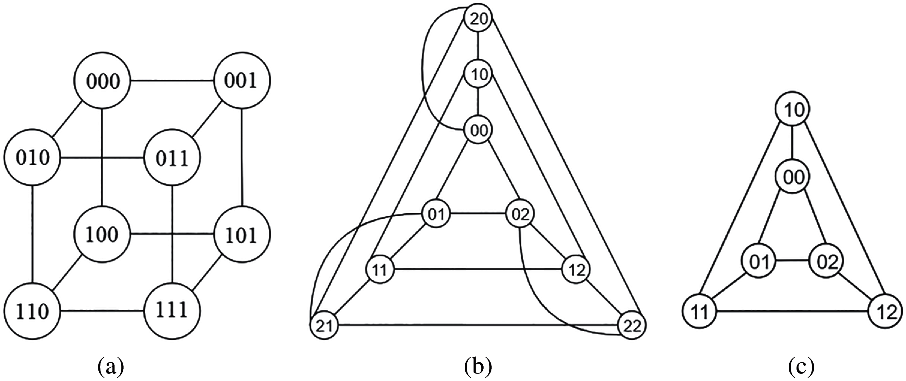
Figure 7: (a) Hypercube Q3 with binary vectors. (b) Hypercube Q3 with ternary vectors (K3 ⋅ K3). (c) Generalized hypercube Q2 using binary and ternary vectors (K2 ⋅ K3)

4.1 Disjoint Partitioning of Arbitrary Graphs to Regular Graphs

All our graph partitioning methods use the quantum Grover’s algorithm. With the benefit of Grover’s algorithm, quantum components of our algorithms gain a quadratic speed up comparing with the standard algorithm for these problems. Symmetric functions in Grover oracles are realized as in Section 2, but below a standard although less efficient realization is used for simplicity.

4.2 Example Oracles for the Hypercube Partitioning Problem

This first our oracle is designed for finding all disjoint partitions of an arbitrary undirected graph to regular graphs. In regular graphs, the degree of every node should be the same, we transform this condition into a Boolean equation and use this equation as a constraint to search all satisfied subsets of vertices in the graph. The E-Regular graphs are found for every value of E separately.

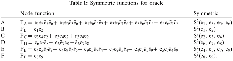
Consider the graph G(V, E) in Fig. 8, V = {A, B, C, D, E, F}, E = {e1, e2, e3, e4, e5, e6, e7, e8, e9}. We want to find all complete partitionings to loops (closed path). Therefore every node has one incoming edge and one outcoming edge, which leads to node with 2-symmetric function S2. We look for all partitions to cycles. Let ei where i ∈ [1, 9] be a Boolean variable corresponding to the edges. If edge ei belongs in a selected regular graph, then ei = 1; otherwise ei = 0. Thus the equations for nodes are as in Tab. 1.

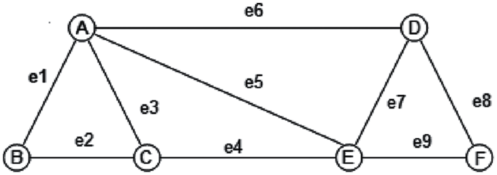
Figure 8: Example graph for partitioning to complete and disjoint sub-graphs

In this example we got two solutions, one is (e1, e2, e4, e9, e8, e6) which is a cycle {A, B, C, E, F, D}, another solution is (e1, e2, e3, e7, e8, e9), this one is two ternary hypercubes (cycles) {A, B, C} and {D, E, F}. To find all complete partitionings we create an oracle that is using a logic AND of node functions for all nodes of the graph. If we want to calculate the solutions with the best costs we need to add a sub-oracle composed from the quantum counter and comparator and we need to repeat calling Grover with modified oracles.

In our oracle, besides the symmetric function blocks, we also use a quantum counter and comparator to save the quantum cost [34] of our circuit. In this example, we have 6 symmetric functions with related nodes. To check the satisfiability of our constraint, instead of using a 7 ⋅ 7 multi-input Toffili gate, we use a counter and comparator in Fig. 9 (mirror circuit not shown for simplification). In general for k nodes of the graph we would need a (k + 1) ⋅ (k + 1) multi-qubit Toffoli gate, we replace it with a counter on log2(k) qubits. Both the quantum cost and the number of ancilia qubits are thus significantly reduced for higher values of k. The counter is only incremented when the symmetric function corresponding to its node is satisfied. The final result of the counter is compared in the equality comparator with the target we want which is 6 our case. If they are equal that means that our constraint is satisfied. The quantum cost of 7 ⋅ 7 multi-qubit Toffoli gate is 125, the cost of our counter and comparator is 87.

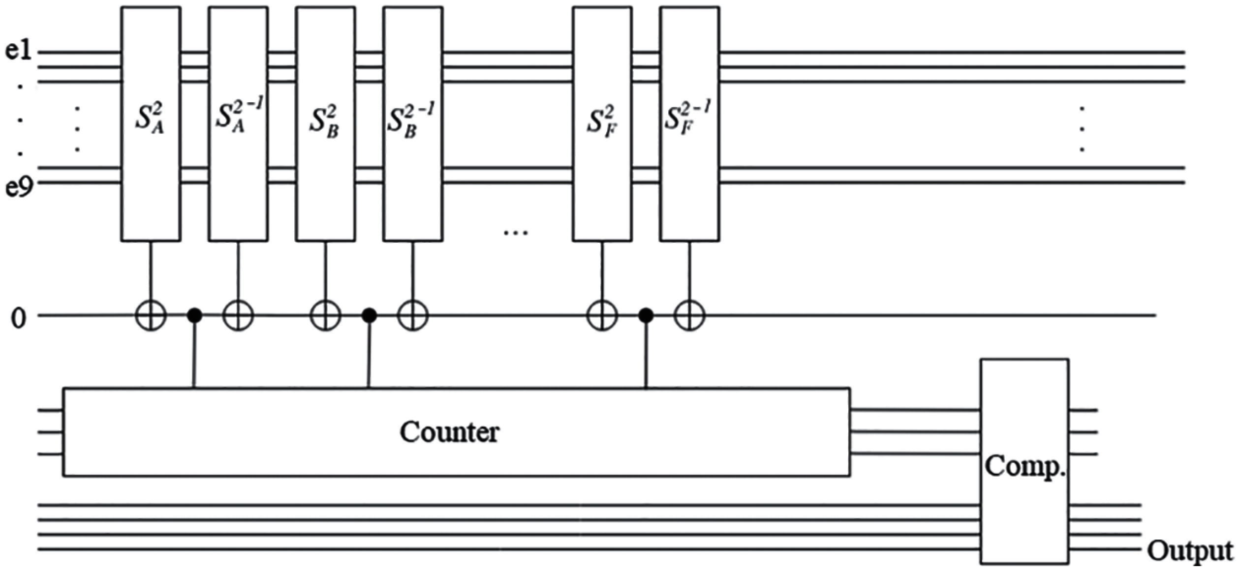
Figure 9: Quantum oracle for graph from Fig. 8

These results were simulated and verified by us using the Qiskit quantum simulator.

4.3 Partial Hypercube Partitioning

In partial hypercube partitioning, we find all subsets of nodes that are sub-hypercubes (cliques) but we allow also to exist nodes that do not belong to any sub-hypercube. Thus for graph from Fig. 8 all individual sub-graphs {A, B, C}, {D, E, F}, {A, C, E}, {A, B, C, E}, and many other will be good solutions. The small modification of oracle is to allow the subsets of nodes, thus to every row of Tab. 1 we add to the node function of node FX additional function S0 of all its adjacent edges. For instance, now we have FC = e3e4̅e2 + e3̅e4e2 + ̅e3e4e2 + (̅e3 ̅e4 ̅e2).

By the property of Lattice structure, the symmetric block is a highly modular design in our algorithm, by adding a specific symmetric function, we can extend symmetric function of the block without generating a new Lattice diagram.

5  Solving DSOP SOP and Minimization Problems for Boolean Functions Using Partial Hypercube Partitioning

Partial Hypercube Partitioning is used to minimize Boolean functions. Normally, SOP minimization is reduced to finding the set of all prime implicants (primes) and next solving the set-covering problem to cover all true minterms with set of primes of the lowest cost. We follow the approach to find DSOP first. For instance in one variant our hybrid algorithm solves the DSOP minimization by finding partitions to large product implicants first and follows with partitions to smaller products. The result is not optimal but we obtain the quadratic speedup to a quantum component of this problem. DSOP can be transformed to SOP equations by enlarging each product implicant to the cheapest prime implicant. This is done by removing subsets of literals from these products, similar as it is done in [18], but this is not a subject of this paper.

DSOP minimization. All minterms included in a product implicant are pairwise compatible so the nodes of these minterms are all pairwise connected by edges in the graph (a clique, a sub-hypergraph). For instance, for a Boolean function specified by the set of minterms 0000, 0001, 0100, 0101, 0111, 0110, 1111, 1110 the minterms 0000, 0001, 0100, 0101 create a clique or a 3-Regular sub-graph that is disjoint from the other 3-Regular sub-graph 0111, 0110, 1111, 1110. This complete partition is a disjoint partition (clique covering) leading to a DSOP solution ̅ac + b c of this function. This is also an optimal SOP, as products ̅ac and bc are disjoint. In another DSOP variant the subgraph {0100, 0101, 0111, 0110} is found which corresponds to prime ̅ab to be next used in covering.

SOP minimization. Every product implicant from the DSOP found is individually extended to the largest prime for SOP using the method from [35]. In rare cases, but only in unspecified Boolean functions, minterms in a clique can be pairwise compatible but not compatible as a group thus they do not create a product implicant. In this case, a special transformation is done to create a SOP or a three-level circuit is synthesized.

Example 1

Given is a Boolean function: F(a,b,c,d)=Σ(1,5,6,7,11,12,13,15), its K-map is presented in Fig. 10.

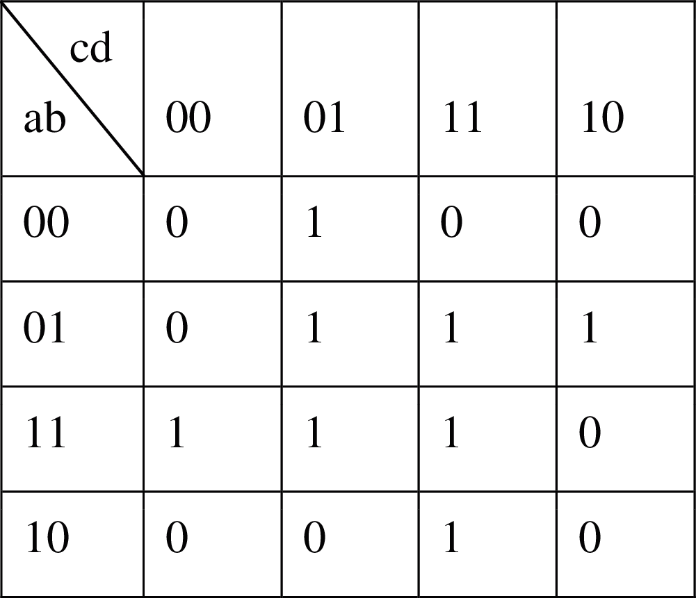
Figure 10: Karnaugh map for function F(a, b, c, d)

Since our quantum algorithm does not fetch data from the input Boolean function directly, we need to use a classical computer for preprocessing and post-processing the data for the quantum Grover’s algorithm.

Step 1. Preprocessing (Classical Computer):

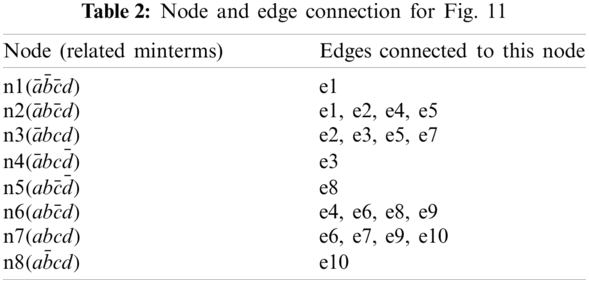
Based on the input function F(a, b, c, d), a compatibility graph is created by a classical computer, every true minterm in F(a, b, c, d) is a node in this graph, minterm a¯ b¯ c¯ d is node n1 in Fig. 11, the detailed node information is in Tab. 2. Next a supercube operation is executed for every two minterms. If the supercube of two minterms doesn’t contain any false minterm, then create an edge between the two nodes that correspond to these minterms. The complexity of this part is based on the number of input variables, for function of m true minterms, the complexity of the preprocessing part is O(m2).

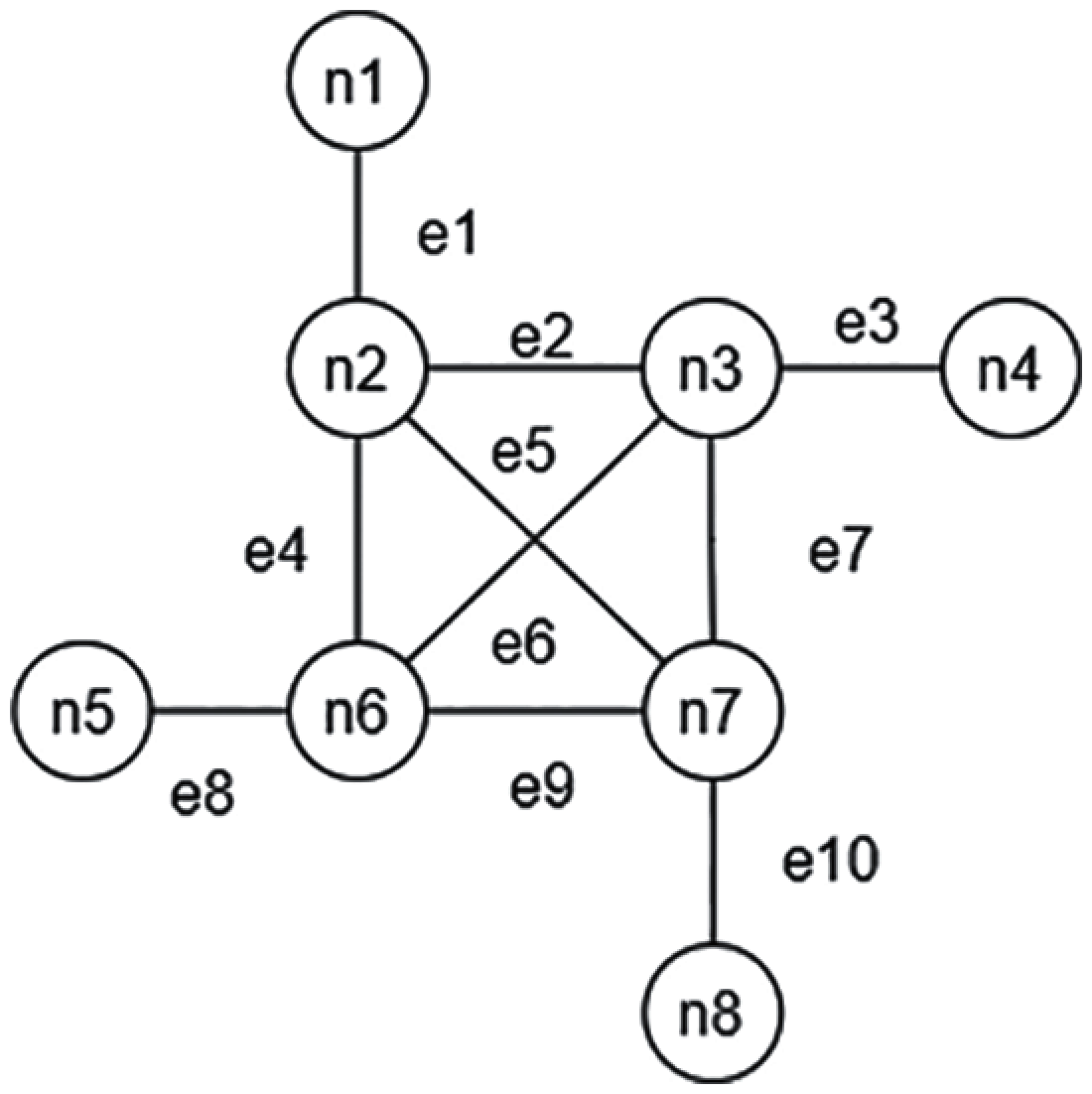
Figure 11: Compatibility graph for function F(a, b, c, d)

After the compatibility graph is created, the hypercube partition quantum algorithm is applied to find all disjoint implicants of F(a, b, c, d). In this case either the complete or the partial hypercube partition can be applied to solve this example, here we choose partial hypercube partition for illustration.

Step 2. Search for DSOP (Quantum Computer).

The indices of symmetric function used in our oracle are defined as (i, 0), where. The variable i is the degree of those nodes that are in majority in the compatibility graph. If the number is 0, i would be assigned to the degree of the second majority node. If there is more than one number of degree majority nodes such as in the example in Fig. 11, in which there is the same number of nodes of degree 1 and degree 4, the index i is chosen from either group of nodes. In this example symmetric indices (1, 0) are selected for demonstration. The second index ‘0’ in the constraint aims to identify the nodes and their connected edges which are not included in the result of the current searching procedure and keep them from being removed by the algorithm.

To find a better solution, both indices can be changed during the multiple calls of Grover’s algorithm. After the result is returned in the first searching, it would be saved in a classical computer, then the classical computer removes this solution from searching space by disabling the related edges at the input of the quantum algorithm. In the next round, the classical computer modifies the first index i in (i, 0), and runs our oracle with the reduced searching space. If no result is found, then index i is changed to the degree of the second majority node and step 2 is repeated until all edges are removed.

Step 3. Post-processing (Classical Computer):

The results of each searching round are saved in the classical computer. When the whole searching process is finished, the DSOP/SOP of this function can be derived by performing a supercube calculation on sets of nodes, as explained below.

In Fig. 11, the initial run of Grover is done by setting the symmetric functions to S0,1 for all nodes. The result of this run is represented in a vector, like (1010000101), which means the edges e1, e3, e8, e10 are selected. With these edges, the classical computer traces back which nodes are selected. In this example the resulting sets of nodes are (n1, n2), (n3, n4), (n5, n6), (n7, n8). After transforming these pairs to the corresponding minterms, for pair (n1, n2) the minterms are ((a¯b¯c¯d), (a¯bc¯d)). Performing the supercube operation on this pair of minterms, the resulting product is a¯c¯d. Similarly, other products from respective sets of minterms are created using supercube operations. (Supercube is an efficient binary operator to find the smallest product of literals that covers its arguments). This way DSOP expression is obtained as F(a,b,c,d)=a¯c¯d+a¯bc+acd. In the second round, the classical algorithm removes the edges: e1, e3, e8, e10 from the graph in Fig. 11. The new graph created by the classical computer and given to the quantum computer is shown in Fig. 12. Let us note that only edges are provided from the standard computer to the quantum computer. Therefore in this case the nodes in the new graph are compiled from edges e2, e4, e5, e6, e7, e9. Thus nodes n1, n4, n2, and n8 presented in Fig. 12 are only for the purpose of explanation. Please note that our hybrid algorithm calls Grover’s algorithm several times with new oracles created on the base of partial results returned from the previous runs of the quantum computer. We found that this principle is applicable to several other problems of logic synthesis in which the existing classical algorithm is converted to a hybrid algorithm based on Grover, in which the quantum algorithm is used only as a subroutine to execute search problems.

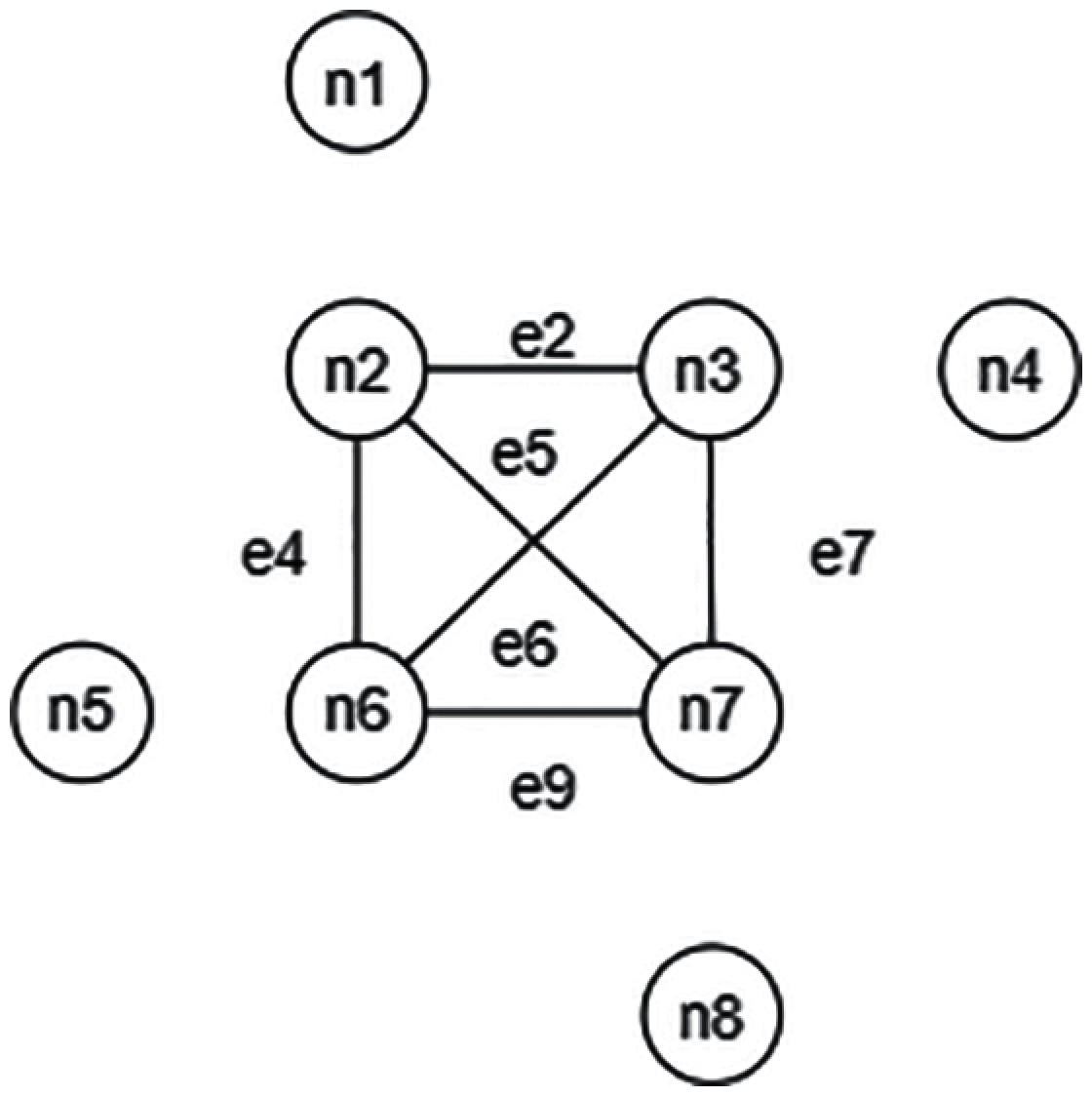
Figure 12: Reduced graph for function F(a, b, c, d)

In the second run, because the degree of majority nodes is 3 (0 is illegal for index i), the indices are changed to (3, 0). Those edges: e2, e4, e5, e6, e7, e9 would be found by symmetric function S3,0, the related minterms are: bd,a¯b¯c¯d,abc¯d¯,ab¯cd¯,a¯bcd¯. Next is to use supercube to check the inclusion of these two results, classical; computer can find the a¯b¯c¯d,abc¯d¯,ab¯cd¯,a¯bcd¯ are included in the first run results, for example the supercube result is abc¯, it means abc¯d¯ is included in abc¯. Another pair (bd, acd), its result is d, there is no inclusion between bd and acd. After removing the edges from the second search, there are no edges left, it means our searching process is finished. Ultimately, the hybrid algorithm finds either SOP:

F(a,b,c,d)=bd+a¯b¯c¯d+abc¯d¯+ab¯cd¯+a¯bcd¯ (6)

or DSOP:

F(a,b,c,d)=a¯c¯d+a¯bc+abc¯+acd. (7)

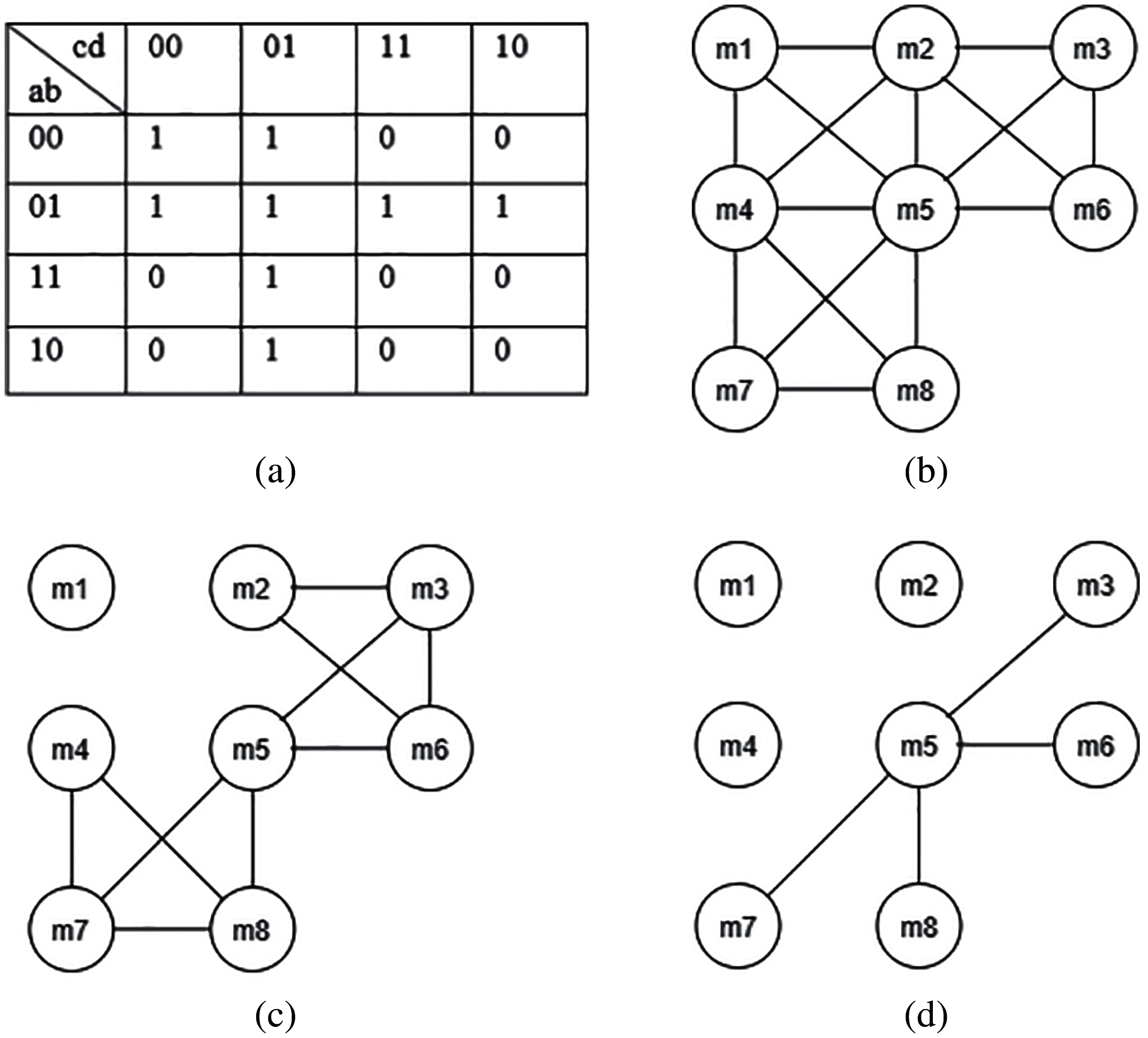
Figure 13: (a) Karnaugh map of Boolean function G(a, b, c, d). (b) Compatibility graph of G(a, b, c, d). (c) Reduced graph after the first search (d) Reduced graph after the second search

Example 2

This example, to minimize function G(a, b, c, d) from Fig. 13a illustrates other properties of our method. Because the degree of the majority nodes is 3, the hybrid algorithm starts with symmetric function S0,3. Under this constraint, there are multiple solutions that can be found, the edges between nodes m1, m2, m4, m5 are selected as a possible solution for illustration. The result of the first search is (a¯c¯,ab¯c¯d,abc¯d,a¯bcd¯,a¯bcd). Fig. 13c is the reduced graph after removing the results of the first run, the degree of the majority nodes is still 3. After applying the constraint with symmetric function S0,3, there is no result found. This is the case that index i needs to be changed to the degree of the second majority node, which is 2. With this modification, multiple results can be found, the same as in the first search. In the example, quantum computer finds the edges, then classical computer transfers edges to nodes (m2, m3, m6) and (m4, m7, m8) for instance, and the result is: (c¯d,a¯b,a¯b¯c¯d¯,a¯bc¯d). Fig. 13d is the reduced graph after removing the edges related to nodes (m2, m3, m6) and (m4, m7, m8). Applying our algorithm with Fig. 13d, the indices are (1, 0). The algorithm keeps the indices as (1, 0) until all product implicants are found. As the final result, the optimal SOP is found: G(a,b,c,d)=a¯c¯+c¯d+a¯b.

6  Conclusion

We developed a hybrid classical/quantum algorithm that uses the Grover’s algorithm in its quantum part. Various quantum oracles constructed here are all based on symmetric Boolean functions that can be efficiently realized in oracles. Our method is applied here to solve two types of hypercube graph partition problems and two types of Boolean function minimization problems. The SOP minimization problem finds multiple applications in classical logic synthesis and PLA (Programmable Logic Array), PAL (Programmable Array Logic), FPGA (Field-Program Gate Array) design. The second, the DSOP minimization problem, is used in classical design as the first step of SOP minimization. DSOP minimization is also used as the first step of ESOP minimization. ESOP minimization is applied in classical logic for synthesis of arithmetic and testing circuits. More importantly ESOP logic is the fundament of minimizing arbitrary quantum functions realized with Inverter, Feynman, and multi-qubit Toffoli gates. Grover’s algorithm gives quadratic speedup when compared to classical counterparts, thus giving promise to future minimization of large functions, also in Machine Learning.

The hybrid algorithm presented above illustrates how several abstract decision and optimization problems can be reduced to Graph Theory problems base on symmetric function. These problems include graph coloring, graph covering, maximum cliques, shortest path, longest path, Traveling Salesman, and domination. Similar methods can be applied to minimization of Exclusive Sum of Product (ESOP) and factorized ESOP expressions. In these problems the concept of compatibility of certain Boolean functions is fundamental and serves to define various partitioning problems to symmetric functions, such as those presented in Sections 1 to 5. Edges are created for pairs of compatible nodes. In addition please note that many interesting and practical problems can be also reduced to some of these Graph Theory problems. For instance, Sudoku Puzzle can be reduced to a graph coloring problem. We believe that there are other fascinating problems in Graph Theory and Topology that would get more efficient solutions with the power of quantum computing.

As far as we know there are no quantum algorithms yet for graph partitionings as defined here. There are also no classical algorithms for the problems formulated and solved in Section 3. There are no quantum algorithms that would solve classical DSOP and SOP minimization as presented in Section 5. These problems, like clique covering and similar, are all NP-hard [36]. The presented methods will become practical with the appearance of quantum computers that can handle more qubits. The usefulness of these algorithms for NISQ (Noisy Intermediate-Scale Quantum) era computing [37] should be also studied.

Funding Statement: The authors received no specific funding for this study.

Conflicts of Interest: The authors declare that they have no conflicts of interest to report regarding the present study.

References

 1.  L. K. Grover, “A fast quantum mechanical algorithm for database search,” in Proc. 28th Annual ACM Symp. on Theory of Computing, USA, pp. 212–219, 1996. [Google Scholar]

 2.  M. J. Ciesielski, S. Yang and M. A. Perkowski, “Multiple-valued boolean minimization based on graph coloring,” in Proc. 1989 IEEE Int. Conf. of Computer Design, USA, pp. 265, 1989. [Google Scholar]

 3.  F. Harary, Graph Theory. Boston, MA, USA: Addison-Wesley Publishing Company, 1969. [Google Scholar]

 4.  M. Schlosser, M. Sintek, S. Decker and W. Nejdl, “HyperCuP—hypercubes, ontologies, and efficient search on Peer-to-Peer networks,” Agents and Peer-to-Peer Computing, vol. 2530, pp. 112–124, 2003. [Google Scholar]

 5.  C. T. Chang, C. Y. Chang and J. P. Sheu, “BlueCube: Constructing a hypercube parallel computing and communication environment over bluetooth radio systems,” Journal of Parallel and Distributed Computing, vol. 66, no. 10, pp. 1243–1258, 2006. [Google Scholar]

 6.  K. O. Stanley, D. B. D’Ambrosio and J. Gauci, “A Hypercube-based encoding for evolving large-scale neural networks,” Artificial Life, vol. 15, no. 2, pp. 185–212, 2009. [Google Scholar]

 7.  E. Chow, H. Madan, J. Peterson, D. Grunwald and D. Reed, “Hyperswitch network for the hypercube computer,” in Proc. of 15th Int. Symp. on Computer Architecture, USA, pp. 90–99, 1988. [Google Scholar]

 8.  S. Bettayeb, “On k-ary hypercube,” Theoretical Computer Science, vol. 140, no. 2, pp. 333–339, 1995. [Google Scholar]

 9.  A. Marquand, “On logical diagrams for n terms,” Philosophical Magazine, vol. 5, no. 12, pp. 266–270, 1881. [Google Scholar]

10. A. Mishchenko and M. A. Perkowski, “Fast heuristic minimization of exclusive-sums-of-products,” in Proceedings of Reed-Muller’2001, Japan, pp. 213–215, 2001. [Google Scholar]

11. N. Song and M. A. Perkowski, “Minimization of exclusive-sum-of-products expressions for multiple-valued input, incompletely specified functions,” IEEE Transactions on CAD, vol. 15, no. 4, pp. 385–395, 1996. [Google Scholar]

12. G. Frank and C. Lane, “Graph isomorphism and adiabatic quantum computing,” Physical Review. A, Atomic, Molecular, and Optical Physics, 2014-02, vol. 89, pp. 22342, 2014. [Google Scholar]

13. A. Frank, A. Kunal, B. Ryan, M. John, Z. Chen et al., “Quantum supremacy using a programmable superconducting processor,” Nature, vol. 574, no. 7779, pp. 505–510, 2019. [Google Scholar]

14. R. J. Trudeau, Introduction to Graph Theory, 2nd ed., New York: Dover Publications, 1994. [Google Scholar]

15. N. Biggs, Algebraic Graph Theory. Cambridge: Cambridge Univ. Press, 1974. [Google Scholar]

16. P. Gao, X. Song, Y. Li and M. A. Perkowski, “Realization of quantum oracles using symmetries of Boolean functions,” Quantum Information & Computation, vol. 20, no. 5&6, pp. 418–448, 2020. [Google Scholar]

17. M. J. Ciesielski, S. Yang and M. A. Perkowski, “Multiple-valued Boolean minimization based on graph coloring,” in Proceedings IEEE Int. Conf. on Computer Design, USA, pp. 265, 1989. [Google Scholar]

18. M. A. Perkowski, “Constraints satisfaction, reversible logic, invertible logic and Grover quantum oracles for practical problems,” in Proc. Reversible Computing 2020, Norway, pp. 3–32, 2020. [Google Scholar]

19. Y. Li, E. Tsai, M. A. Perkowski and X. Song, “Grover-based Ashenhurst–Curtis decomposition using quantum language quipper,” Quantum Information & Computation, vol. 19, no. 1&2, pp. 35–66, 2018. [Google Scholar]

20. A. Gilyén, S. Arunachalam and N. Wiebe, “Optimizing quantum optimization algorithms via faster quantum gradient computation,” in Proc. 13th ACM-SIAM Symp. on Discrete Algorithms, CA, USA, pp. 1425–1444, 2002. [Google Scholar]

21. D. Maslov and G. W. Dueck, “Improved quantum cost for n-bit Toffoli Gates,” Electronic Letter, vol. 39, no. 25, pp. 1790, 2003. [Google Scholar]

22. M. A. Perkowski, M. Chrzanowska-Jeske and Y. Xu, “Lattice diagrams using Reed–Muller logic,” in Proc. of Reed-Muller’97, U.K., pp. 85–102, 1997. [Google Scholar]

23. M. Lukac, D. Shah, M. A. Perkowski and M. Kameyama, “Synthesis of quantum arrays from Kronecker functional lattice diagrams,” IEICE Transaction on Information and System, vol. E97, no. 9, pp. 2262–2269, 2014. [Google Scholar]

24. S. B. Akers, “A rectangular logic array,” IEEE Transactions on Computer, vol. C-21, no. 8, pp. 848–857, 1972. [Google Scholar]

25. T. Sasao and J. Butler, “A design method for look-up table type FPGA by pseudo-Kronecker expansion,” in Proc. on 24th Int. Symp. on Multiple-Valued Logic, Boston, USA, pp. 97–106, 1992. [Google Scholar]

26. R. Babbush, G. Craig, B. Dominic, W. Nathan, “Encoding electronic Spectra in quantum circuits with linear T complexity,” Physical Review, vol. 8, no. 4, pp. 041–015, 2018. [Google Scholar]

27. M. A. Perkowski, A. Mishchenko and M. Chrzanowska-Jeske, “Generalized inclusive forms—new canonical Reed–Muller forms including minimum ESOPs,” VLSI Design, vol. 1, pp. 13–21, 2002. [Google Scholar]

28. A. Paler, L. M. Sasu, A. Florea and R. Andonie, “Machine learning optimization of quantum circuit layouts,” arxiv 2007.14608v1 [quant-ph], 29 July 2020. [Google Scholar]

29. M. A. Perkowski, M. Lukac, D. Shah and M. Kameyama, “Synthesis of quantum circuits in linear nearest neighbor model using positive Davio lattices,” Facta Universitatis, Electronic Energetics, vol. 24, no. 1, pp. 73–89, 2011. [Google Scholar]

30. V. P. Suprun and D. A. Gorodecky, “Matrix method of polynomial expansion of symmetric Boolean functions,” Automatic Control and Computer Sciences, vol. 47, no. 1, pp. 1–6, 2013. [Google Scholar]

31. W. H. Mills, “Some complete cycles on the n-Cube,” in Proc. of American Mathematical Society, MA, USA, pp. 640–643, 1963. [Google Scholar]

32. J. Zhou, Z.-L. Wu, S.-C. Yang and K.-W. Yuan, “Symmetric property and reliability of balanced Hypercube,” IEEE Transactions on Computers, vol. 64, no. 3, pp. 876–881, 2015. [Google Scholar]

33. F. Harary, J. P. Hayes and H. J. Wu, “A survey of the theory of hypercube graphs,” Computers & Mathematics with Applications, vol. 15, no. 4, pp. 277–289, 1988. [Google Scholar]

34. D. Maslov and G. W. Dueck, “Improved quantum cost for n-bit Toffoli gates,” Electronic Letter, vol. 39, no. 25, pp. 1790, 2003. [Google Scholar]

35. G. Yang, X. Song, H. William and M. A. Perkowski, “Fast synthesis of exact minimal reversible circuits using group theory,” in Proc. of the 2005 Asia and South Pacific Design Automation Conf., China, pp. 1002–1005, 2005. [Google Scholar]

36. Ch. Umans, T. Villa and A. Sangiovanni-Vincentelli, “Complexity of two-level logic minimization,” IEEE Transactions on CAD, vol. 25, pp. 1230–1246, 2006. [Google Scholar]

37. J. Preskill, “Quantum computing in the NISQ era and beyond,” Quantum, vol. 2, pp. 79, 2018. [Google Scholar]

This work is licensed under a Creative Commons Attribution 4.0 International License, which permits unrestricted use, distribution, and reproduction in any medium, provided the original work is properly cited.