DOI:10.32604/cmc.2022.020044
| Computers, Materials & Continua DOI:10.32604/cmc.2022.020044 | |
| Article |
Machine Learning Approaches to Detect DoS and Their Effect on WSNs Lifetime
1College of Computing and Informatics, Saudi Electronic University, Riyadh, 11673, Saudi Arabia
2The School of Information Technology, Sebha University, Sebha, 71, Libya
*Corresponding Author: Rami Ahmad. Email: r_a_sh2001@yahoo.com
Received: 07 May 2021; Accepted: 08 July 2021
Abstract: Energy and security remain the main two challenges in Wireless Sensor Networks (WSNs). Therefore, protecting these WSN networks from Denial of Service (DoS) and Distributed DoS (DDoS) is one of the WSN networks security tasks. Traditional packet deep scan systems that rely on open field inspection in transport layer security packets and the open field encryption trend are making machine learning-based systems the only viable choice for these types of attacks. This paper contributes to the evaluation of the use machine learning algorithms in WSN nodes traffic and their effect on WSN network life time. We examined the performance metrics of different machine learning classification categories such as K-Nearest Neighbour (KNN), Logistic Regression (LR), Support Vector Machine (SVM), Gboost, Decision Tree (DT), Naïve Bayes, Long Short Term Memory (LSTM), and Multi-Layer Perceptron (MLP) on a WSN-dataset in different sizes. The test results proved that the statistical and logical classification categories performed the best on numeric statistical datasets, and the Gboost algorithm showed the best performance compared to different algorithms on average of all performance metrics. The performance metrics used in these validations were accuracy, F1-score, False Positive Ratio (FPR), False Negative Ratio (FNR), and the training execution time. Moreover, the test results showed the Gboost algorithm got 99.6%, 98.8%, 0.4% 0.13% in accuracy, F1-score, FPR, and FNR, respectively. At training execution time, it obtained 1.41 s for the average of all training time execution datasets. In addition, this paper demonstrated that for the numeric statistical data type, the best results are in the size of the dataset ranging from 3000 to 6000 records and the percentage between categories is not less than 50% for each category with the other categories. Furthermore, this paper investigated the effect of Gboost on the WSN lifetime, which resulted in a 32% reduction compared to other Gboost-free scenarios.
Keywords: WSN; intrusion detection; machine learning; DoS attack; WSN security; WSN lifetime
Wireless network technology is the main nucleus in the development of the Internet of Things (IoT). That is because wireless networks are the main key in the transfer of interactive data between devices and humans or devices-to-devices [1]. These devices are part of automation and control systems, embedded systems, Wireless Sensor Networks (WSN) and others that share their information in various environments without need of human intervention. Each application using these devices mostly consist of three layers, which comprise; the perception, the network and the application [2]. Application and network layers are mostly executed in high-power devices, while the perception layer is executed in low-power devices to keep them running for as long as possible, especially with the use of limited battery life systems.
The perception level consists of several WSN nodes that communicate with each other using various radio frequencies that are capable of performing different sensing, recording, calculating, and tracking activities [3]. These WSN nodes are considered as mini-computers that are characterized by low computing speed, restricted bandwidth, limited memory space, and limited battery life. In addition, 6LoWPAN and Zigbee are two protocols used extensively in WSN networks in between physical layer and Media Access Control (MAC) layers of IEEE 802.15.4 [4].
However, since the WSN nodes are designed to operate in various untrusted surroundings, which are not periodically monitored. This makes the WSN nodes vulnerable to various security attacks, especially if they are related to important and sensitive data [5]. Moreover, with regards to WSN nodes boundaries, i.e., CPU power and energy [6], it is sometimes difficult to provide a charger for them in these conditions. Therefore, the drawbacks of WSN nodes and their dependence on public wireless networks contribute to many problems in the WSN architecture. One of these issues applies to security, privacy, and availability in the perception layer. In the area of security, the main issue is protecting the data connection between WSN nodes against spoofing and eavesdropping by illegal WSN node modification alteration [7,8]. In WSN node availability, via sinkhole, wormhole, Sybil, hello flood, and Denial of Service (DoS) attacks, an attacker can disable it by interfering with data packet transmission [3]. DoS attacks can waste WSN nodes resources and lose their data packets within the networks. Therefore, in this paper, we will focus on slowing down Distributed (DDoS) and DoS in WSN networks within minimum power consumption and good accuracy in defining both attacks [9]. Moreover, DoS or DDoS attacks focus on depleting WSN node resources through allowing them to receive unnecessary or authorized packets for that WSN node. These events force WSN nodes to reject the network's services to the legitimate WSN nodes, and this type of attack can occur in any layer of WSN model system [10].
Due to the risk of this type of attack on WSN networks, intrusion detection technique is the best defense for DDoS attacks [11]. Intrusion detection is divided into signature-based and anomaly-based. In anomaly pattern, the technique needs to monitor network connectivity in a regular manner and compare the ongoing WSN networks activities with the current normal behaviour traffics [9,11]. Therefore, various techniques have been used to improve the performance of DoS detection in both active and passive methods. Supervised machine learning algorithms are one such technique used to predict and classify DDoS attacks. The Logistic Regression (LR), decision Tree (DT), artificial neural networks, Support Vector Machine (SVM), deep learning, and K-Nearest Neighbour (KNN) are common algorithms for this [12]. The authors in [1,2,13–17] used different techniques related to deep learning mechanism, and their results regarding to detection accuracy, mean squared error, and sensitivity showed good performance, but none of them discussed the effect of their proposal on WSN networks such as nodes power consumption and network lifetime. Moreover, other publications were using regular networks traffic datasets instead of WSN nodes datasets [18]. Other algorithms for detecting DDoS have been proposed in [19], the work used authentication policy to remove DoS attacks by splitting the WSN nodes into clusters and linking all cluster WSN nodes in a single authentication message. In addition, the work in [20,21] showed that machine learning techniques (LR, SVM, and DT) are suitable for real-world deployment rather than deep learning mechanism, because deep learning algorithms need massive training data in order to be able to give high-accuracy results in classification process. Therefore, the process of implementing these capabilities on training operations via the WSN network node is a waste of time and effort [14].
A different other technique related to the incorporation of WSN nodes clustering mechanism and machine learning in DDoS detection has been proposed in [22,23]. Furthermore, the authors in [24] used a SVM based on spatiotemporal and attribute correlations on data collected from WSN nodes. However, no publication has yet discussed the effect of the above algorithms on WSN networks using the same simulation and dataset. Furthermore, as the WSN nodes have limited power and CPU, anti-DDoS measures should be simple and fast. Therefore, the main contribution to this work is the use of new WSNs environments with performance analysis of the machine and deep learning algorithms of the WSN network dataset as well as their effect on WSN network lifetime. The major contributions of this work are summarized as follows:
(1) We proposed a new WSN network environment which combined WSN nodes clustering technology, authentication, key management [25] and WSN-Dataset [23] to help detect DoS attacks and study the effect of this detection on WSN node power consumption.
(2) Analyzing the effect of dataset size on performance of machine learning classification techniques. The original dataset was divided into different subsets, decreasing in size (number of records).
(3) Analyze the effect of DoS anomaly detection performance on WSN network lifetime.
The remainder of our paper is organized as follows. Section 2 provides an overview of related work in WSN networks, DoS attacks, and machine learning techniques. Section 3 explains methodology, environmental development, the cluster management, the machine learning test and the decision-making. Section 4 discusses data collection and organization. Section 5 discusses implementation and evaluation for complexity analysis in machine learning techniques and WSN networks lifetime. Finally, the conclusion and future work of the paper is given in Section 6.
2 Background and Related Works
In this section we will provide a literature review and technical background for the WSN networks and clustering efficiency in WSN networks, intrusion detection in WSN networks, and machine learning algorithms in intrusion detection.
WSN network is a radio access spectrum that uses 2.4 GHz which is designed to work in low power, low range, and low processor circumstances. The Internet Engineering Task Force (IETF) standardized it under the name of IEEE 802.15.4 [26]. Moreover, the Zigbee and 6LoWPAN are two protocols used to manage WSN networks and transfer data to Access Point (AP). Both protocols use the Media Access Network (MAC) and physical IEEE 802.15.4 (Perception) layers as illustrated in Fig. 1. Meanwhile, the difference between them is the 6LoWPAN introduces IPv6 and Low Power and Lossy Networks (RPL) protocol to capture WSN nodes and forward their data to edge AP [27].
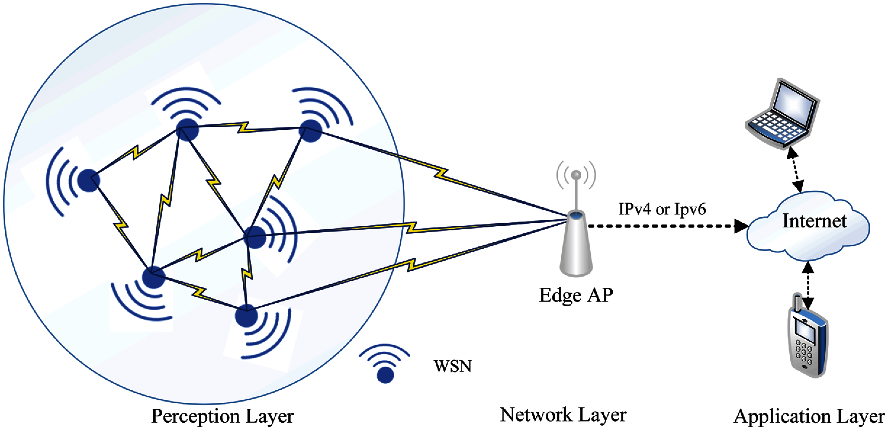
Figure 1: The architecture of WSN networks [26]
As shown in Fig. 1, the WSN networks are responsible for drawing the network topology and routing table in the perception layer using different protocols [26] as explained earlier. Each WSN node associates with the set of its neighbouring peers WSN nodes, then the WSN node starts collecting data from different locations and forwarding the data to the network layer (edge-AP). This process of routing is done either using RPL protocol in 6LoWPAN or Distance Vector (DV) protocol in Zigbee. For data transmission protocol, a User Datagram Protocol (UDP) is used to reduce the packet's complexity and reduce CPU overhead. Moreover, to secure data transmission over UDP, the Datagram Transport Layer Security (DTLS) protocol is used on top of UDP [28].
As mentioned previously, the main objective of the DDoS attack is to affect the network's availability by disrupting services and network performance. Therefore, the effect of this type of attack varies by each network layer stack [7]. Since wireless sensor networks have five network layers stack, each layer has a different type of attacks [11,29]. The attached Tab. 1 shows each layer and type of DoS it represents.

The Blackhole and Grayhole DDoS attacks affect the routing protocol in layer three by declaring the attacker node itself as the cluster head, and we will discuss the cluster head functionality in detail in the clustering management subsection. Whereas, the Flooding attack affects the WSN network availability by sending a large number of advertising messages to cluster heads. In a scheduling attack (e. Time-Division Multiple Access (TDMA)), the effect is related to physical and MAC layers’ activity by changing the broadcast channel schedule to unicast channel schedule. This change leads to packets collision and later data loss [23].
Numerous researchers try to reduce DDoS or DoS in WSN networks. In [19], the authors used the Message Authentication System (MAS) algorithm to localize and remove DoS. The proposal divides the WSN nodes into various clusters and each cluster head uses the MAS algorithm to distinguish between legitimate and phishing messages. In [30,31], the authors refined the k-means clustering scheme for detecting DDoS and misdirection attacks. In [32], the authors used user-behaviour learning analysis in a home WSN network to detect abnormal attacks. Furthermore, authors in [16] used Restricted Boltzmann Machine-based Clustered IDS (RBC-IDS), a deep learning-based methodology to track critical infrastructure using three hidden layers for potential intruders. Furthermore, authors in [33] used Genetic algorithm with Multi-Layer Perceptron (MLP) to enhance anomaly detection performance. Authors in [23] created a dataset for WSN networks and used an artificial neural network algorithm to detect and classify four types of DoS attacks. Moreover, in [34], the authors proposed an optimization algorithm called an adaptive-chicken swarm to cluster WSN nodes and then used a VSM classifier to detect DoS attacks in each cluster. However, this work will focus on analysing DoS attacks detection performance rather than anti-attacks measures.
2.3 Machine Learning in Intrusion Detection Approach
Machine learning is the mechanism that automatically enhances or learns from an analysis or experience and works without directly configuring it. Its divide between supervised and unsupervised learning. Supervised learning characterized into classification and regression.
Classification is categories into statistical learning (SVM and Bayesian), logic-based (DT), instance-based (KNN), and perceptron-based (Recurrent Neural Network (RNN), Long Short Term Memory (LSTM), Convolutional Neural Network (CNN), MLP, and artificial neural networks). In addition, the main responsibility of this type of learning technique is to create a model that describes the relationships and dependency ties between input features and expected objective outcomes [12]. Therefore, supervised learning can solve various problems of the WSN network, fault and anomaly detection being one of them. Tab. 2 depicts various categories of detection approaches and machine learning techniques that are used in detection attacks in WSN networks.

In a simple review of the functioning of supervised algorithms, which we will deal with in this study, the KNN works based on the manifold hypothesis. If the majority of the neighbors of the sample are from the same class, then the sample is likely to be from that class as well. As a result, the categorization outcome is limited to the top-k closest neighbors. The efficiency of KNN models is heavily influenced by the parameter k. The smaller k, the more complicated the model is, and the greater the chance of overfitting. The bigger k, on the other hand, the simpler the model and the lower the fitting ability [43]. Moreover, the Naïve Bayes works on the basis of probability distribution and the trait independence hypothesis. The probability distribution for distinct classes are calculated for each sample, then the maximum probability class is assigned to the sample [11,29]. The probability distribution is illustrated as Eq. (1).
where P is the probability of class Ckproducing the term xi..
Another classifier that will be considered in our work is the DT, which works on the basis of the chain of rules in the tree topology. The tree topology gives it the speed to exclude the redundant features and generate child nodes from the root node. However, some advanced algorithms, such as Random Forest and Gboost, consist of multiple decision trees [42]. In the linear model, the LR technique is considered a variant of it, and the probabilities of different classes are calculated using the parametric logistic distribution, which is shown in Eq. (2) [29]
where sample x is categorized in the extreme probability class.
Moreover, in our work we also used another type of traditional supervised algorithm named SVM. In SVMs, the goal is to locate a maximum-margin separating hyperplane in the n-dimensional feature vector. Since the separation hyperplane is controlled by a small number of service vectors, SVMs can produce satisfying results even with small-scale training data. SVMs, on the other hand, are susceptible to noise around the hyperplane [12].
In deep learning technology, the MLP uses the propagation learning in two phases: forward and back during the training phase. In the forward neural step, input data is given to each neuron of the hidden layer. The activation value of each hidden neuron and output node is calculated. An error is generated by the disparity between the output target and the specific target value. The error is propagated back from the output layer to the input layer in the back-propagation step, and weights between output neurons and hidden neurons are changed. Weights are updated using the gradient descent approach [44]. Moreover, another different type of deep learning that also uses backpropagation is LSTM. It is an automated development of a RNN through facilitating memory recall of previous data. Moreover, LSTM solved the vanishing gradient problem found in RNN. LSTM is well suited for classifying, processing and forecasting time series due to time delays of unknown duration [17].
However, in this paper we will analyze the WSN networks traffic based on aforementioned machine learning classifications to see how it performs in detecting DoS attacks on WSN networks.
3 Methodology and Environmental Development
The proposal environment consists of three processes. The first is to aggregate WSN nodes to multiple clusters and each cluster has Cluster Head (CH) in a mobile WSN nodes environment. In the following process, a Machine Learning Testing (MLT) approach is used to analyse traffic in each CH node to distinguish between normal and abnormal coming packets. In the last process, CH will make a decision based on the second process results. The overall architecture of our proposal is depicted in Fig. 2.
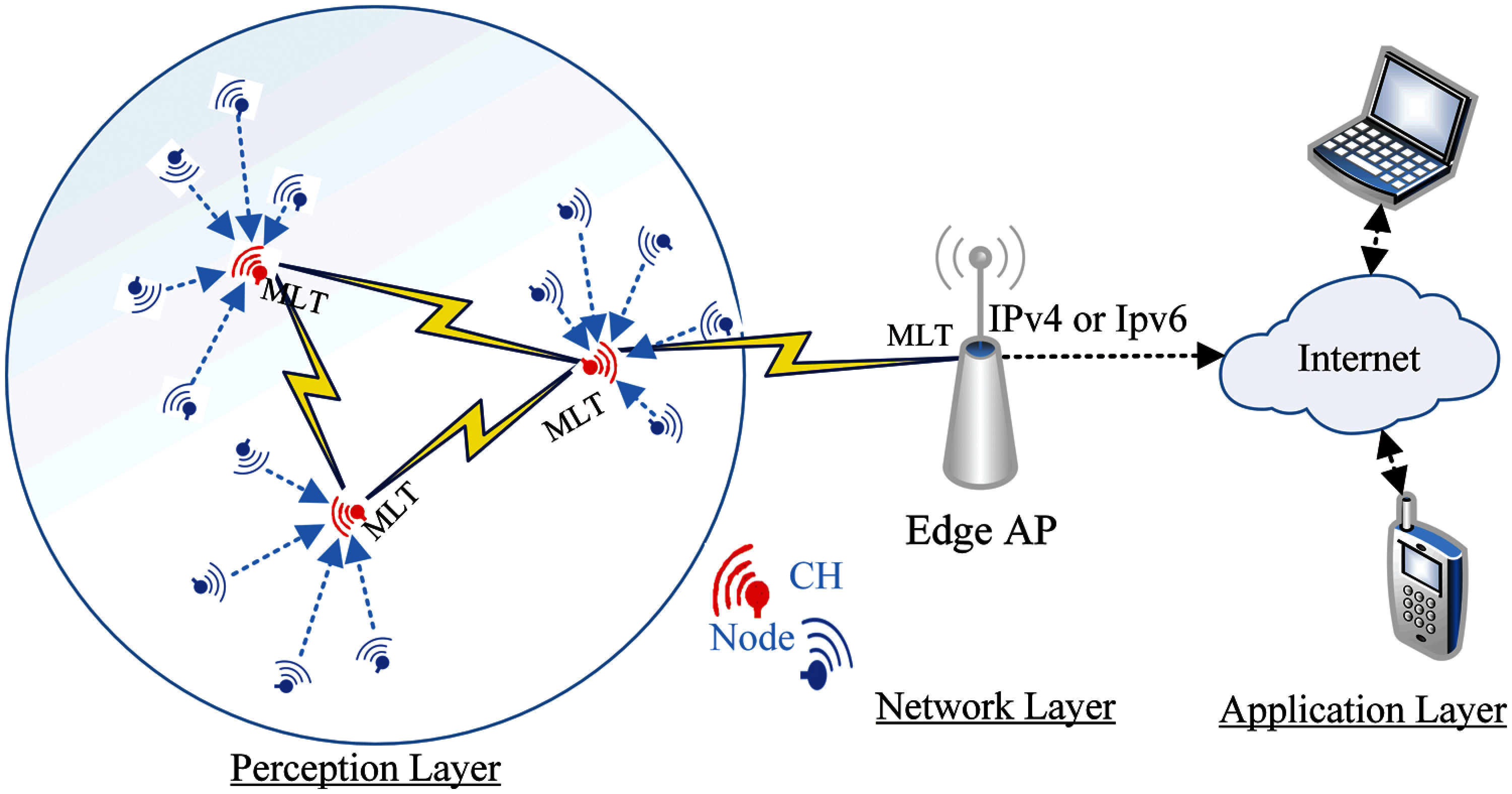
Figure 2: The proposed WSN networks environment
As depicted in Fig. 2, the WSN nodes (n1, n2,…, nN), where N is the number of WSN nodes within the Edge AP. The WSN nodes sense the environment and collect relevant data. Then the sensed data are sent to the Edge AR via the CH. The WSN nodes are assumed to be mobile and can move in different directions. At the beginning, the CH is chosen based on several criteria such as the WSN node energy, the distance between the nodes and the number of neighbouring nodes. Once the CH is chosen and the clusters are formed, data begins to be transmitted and the CH starts analysing it.
Cluster technology contributes to reducing the energy consumption of WSN nodes by choosing the appropriate neighbouring WSN node to transmit data through it to AP. Thus, the transmission and reception of data from the neighbouring nodes, which has weak signal strength to increase the power consumption in both WSN nodes (transmitter and receiver). Therefore, many studies have used different combinations of techniques in selecting CH such as [34,45,46,15–17], but most of them do not have an optimal solution. In this work we will use the clustering management that was proposed in [25]. Their proposal is based on the low complexity calculation and supports the WSN nodes mobility. However, we will alter their clustering algorithm to cover minimum and maximum of ordinary WSN node numbers in each cluster to avoid complexity analysis in each CH. The altered clustering algorithm is presented in Fig. 3.
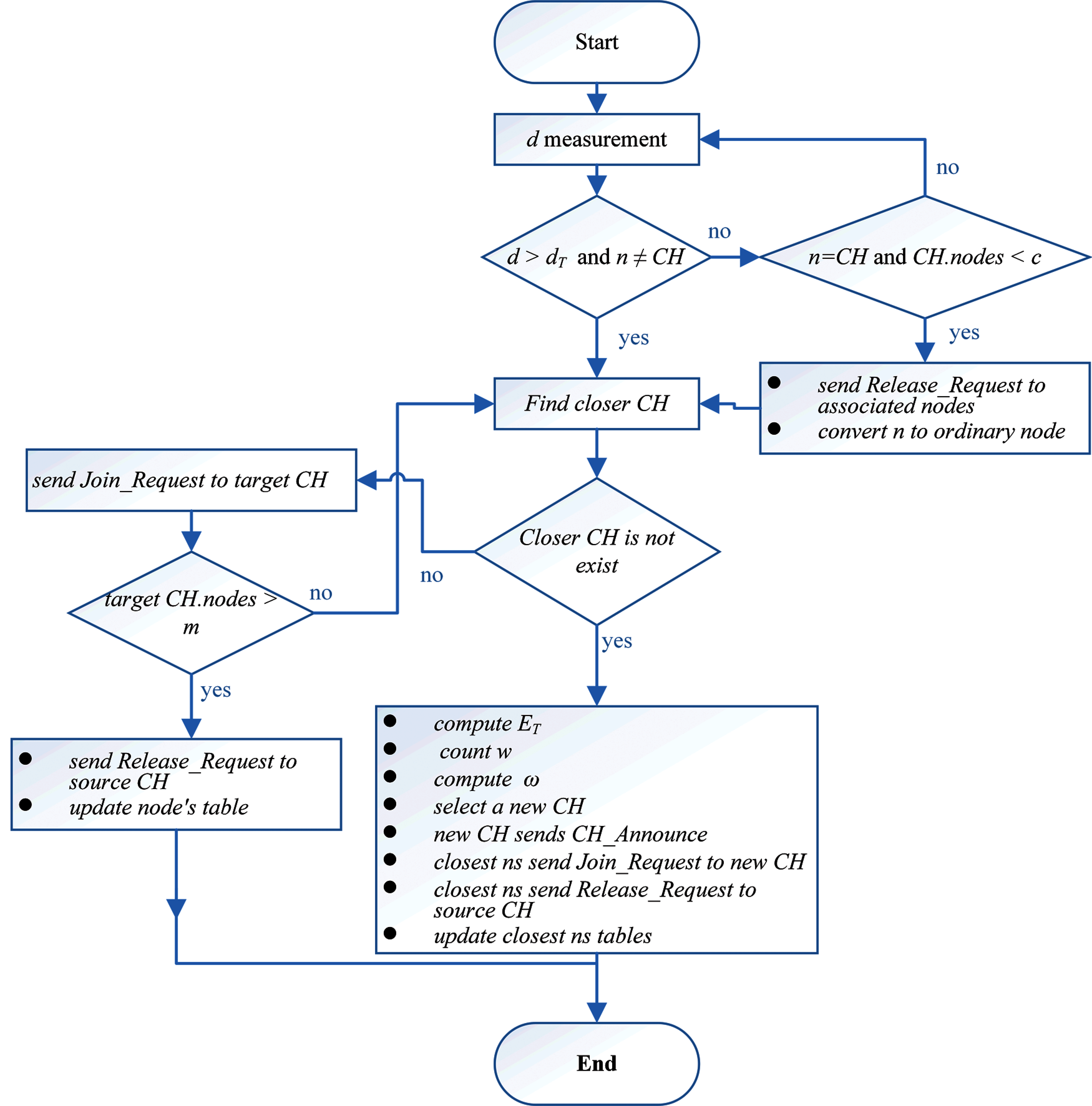
Figure 3: The clustering management algorithm [25]
The parameters d, dT, ET, w, and ω represent the distance between WSN nodes, the distance threshold, the WSN node energy threshold, the average distance between candidate CHs and adjacent nodes, and the weight of CHs selection, respectively by the flowchart. However, all these parameters were explained in detail in [25]. The algorithm starts by continuous verification (period of time) of the distance between each WSN node (n) and its CH. Since the WSN nodes are moving at a low speed of about 5 m/s, the distance will be checked once per second [47]. If the distance begins to approach the distance threshold value (dT), the WSN node begins to search for the closest CH to pair with it. A WSN node sends a Join_Request message to target the CH, then sends the Release_Request message to its source CH. This process uses WSN mobile nodes that lead to the reassembling and regrouping process. For instance, the n moves away from the linked CH and when the distance between them becomes less than dT, n starts looking for the nearest CH, if there is no close CH, n initiates the process of creating a new CH between the adjacent WSN nodes and then asks them to join. On other hand, if the CH moves away from its linked WSN nodes, it has a few of them (c), where c is the lower WSN nodes number that are linked with each CH. CH will release the linked WSN nodes and become a regular WSN node in order to join to the nearest CH. In addition, the released WSN nodes will also search or create new cluster groups. The last scenario is when the CH has a number (m) of linked ordinary WSN nodes, in which case the target CH will not accept the new connection and the WSN node starts to repeat the same scenario to find a closer CH or to create a new CH group.
3.2 Machine Learning Testing Approach
In this step of our proposal environment, we select various machine learning classification schemes such as KNN, LR, SVM, Gboost, DT, Naïve Bayes, LSTM, and MLP. Next, we train these algorithms through the WSN traffic dataset [23] that we chose and then test. The algorithm that has the best performance metrics will be determined to be a MLT approach (see Fig. 4) in each CH node.
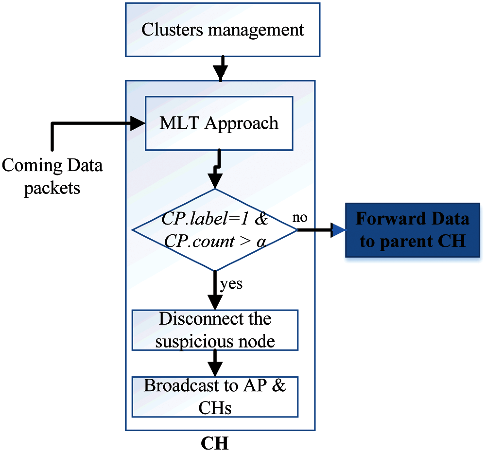
Figure 4: Make a decision in each CH
At this process of our proposal environment, the CH monitors the number of duplicate suspicious packets, if there is a confirmation of duplication, the CH node will cut off the connection with the suspicious WSN node, add WSN node information to its blacklist, and send a broadcast message to the all neighbour CHs and AP informing them about the suspicious WSN node information. This process is illustrated in Fig. 4.
Based on Fig. 4, each data Packet that Comes (CP) will be scanned, if it is labelled as 1, CH will count it as a suspicious packet and then count the number of times it repeats for a period of time. Next, if the CP.count exceeds α (threshold value), the CH will execute the broadcast command and disconnect the connection with that MAC node, where α is the maximum number of suspicious beam at time (t). This process gives an opportunity to reduce the false negative rate in our work by confirming the attack process.
In this work, we are testing it using the WSN network dataset. In network traffic datasets there are three types: the CICDDoS2019 [48], BoT-IoT [49], and WSN-DS [23]. However, the CICDDoS2019 and BoT-IoT were collected from different device types (servers, sensors, routers, and switches) while the WSN-SD was collected from the WSN network environment whose environment is close to ours. WSN-SDcontains four different classes based on the DoS attack types: Flooding, Blackhole, Grayhole, TDMA, and Normal. As with our goals to reduce node power consumption and move the defense decision to Edge AP, we are converting these four types of DoS attacks into one class that is labelled as “1” and the label “0” will be normal. In addition, the WSN-SD was collected through the LEACH routing protocol which is different from standard RPL, however this dataset still works with our modified clustering management algorithm. As the WSN-SD dataset contains 19 features, we have removed five of them (id, time, distance to CH, distance to base-station, and data sent to base-station) to be compatible with our environmental approach.
Moreover, we are spitted the WSN-DS dataset into six different subsets to see the effect of data size on the performance of machine learning algorithms. The first dataset contains all records of the original dataset. As illustrated from Tab. 3, the attacked data is less than normal data by 88.6%. Furthermore, this percentage of the attacking data is distributed as 33% Blackhole, 11% Flooding, 35% Grayhole, and 21% TDMA. Therefore, in the rest of datasets we will look at these ratios to keep the same context.
The second dataset is discounted 40% from the original WSN-DS dataset in each label category, as each category contains different data records. The third dataset is 40% discounted from the second dataset in each label category. The fourth and fifth datasets are divided between normal and attacked in a two-to-one ratio to allow analysis of the effect of the ratios of each category on the training process. In dataset number six, records are divided between the two in a one-to-one ratio due to the small number of records. The WSN-DS datasets description is illustrated in Tab. 3.

5 Implementation and Evaluation
In this section, we first discuss analyzing machine learning schemes in different WSN-DS datasets. The simulation environment and experimental performance are discussed in relation to machine learning algorithms, and then their results are analysed. In the second analysis, it will be applied based on the best machine learning test algorithm that came out from the first analysis to show its effect to the WSN network lifetime.
5.1 Complexity Analysis for Machine Learning Approaches
5.1.1 Experimental Environment
In this analysis, Python3.8 platform is used within Jupyter Notebook software [50] and they operate on a Dell machine with a 1.8 GHz Intel Core i5 processor, 6MB cache, and 8 GB RAM. Operating System is Ubuntu 19.4. The hyper parameters for these analyses are shown in Tab. 4.

5.1.2 Experimental and Performance Metrics
In this work, five performance metrics are utilized to analyse machine learning algorithms on WSN-SD Datasets in different classification categories. The aims are the highest number of True Positive (TP) and True Negative (TN) and low number of False Negative (FN) and False Positive (FP). The number of TN indicates that the normal flows are expected as valid traffic, while the TP is the likelihood of the irregular traffic being labelled as abnormal traffic. Furthermore, the FN illustrates the likelihood of attack flows that are known as normal flows, while the FP represents the likelihood of normal flows predicted as attack flows. The False Positive Rate (FPR) indicates the wrongly defined attack ratio and the inverse False Negative Rate (FNR) over the cumulative sum of the incorrect forecast. In addition, accuracy is the percentage of accurate model prediction for all types of predictions produced. Execution time represents the time taken in the training process, measured in seconds. Moreover, F1-score is used to comprehensively measure the accuracy of the model. The following Equations represent all of the performance metrics used in this analysis:
The Percentage Value (PV) will measure accuracy and F1-Score against the optimal value which is (1), and it will measure FPR and FNR against the optimal value which is (0).
In subsequent analyses, we will review the results of the performance metrics of the machine learning algorithms that we selected on the split WSN-DS datasets in Section 4, namely D1 to D6. Figs. 5–12 show the effect of dataset size on machine learning algorithms. However, SVM algorithms did not respond to the large datasets such as D1 and D2, and thus, no performance metrics were found regarding these two dataset groups. Moreover, in Naïve Bayes technique, there are three types of algorithms (Bernoulli, Multinomial, and Gaussian), we chose a Multinomial algorithm because it provided the best results for performance metrics on the same WSN-DS dataset.
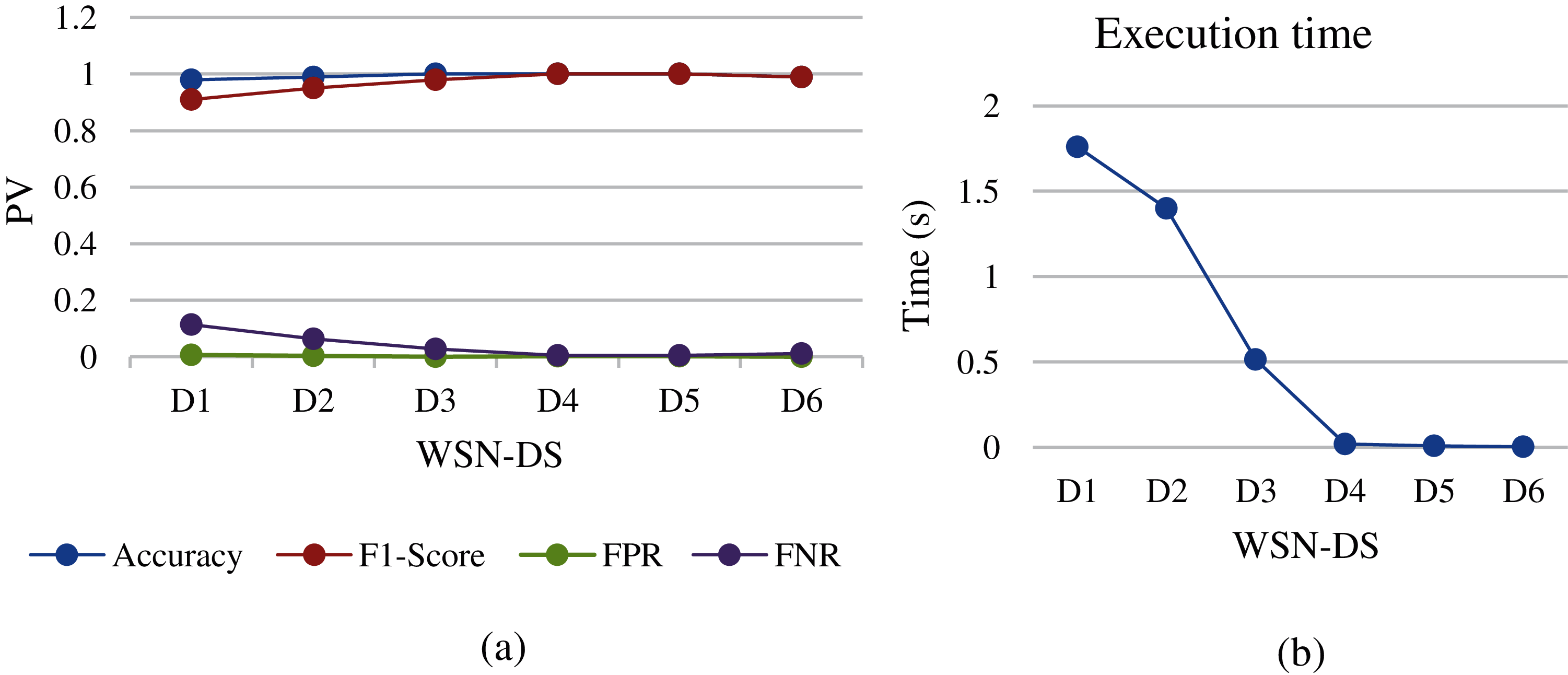
Figure 5: KNN analysis of different WSN-DS dataset sizes: (a) performance metrics, (b) execution time

Figure 6: LR analysis of different WSN-DS dataset sizes: (a) performance metrics, (b) execution time
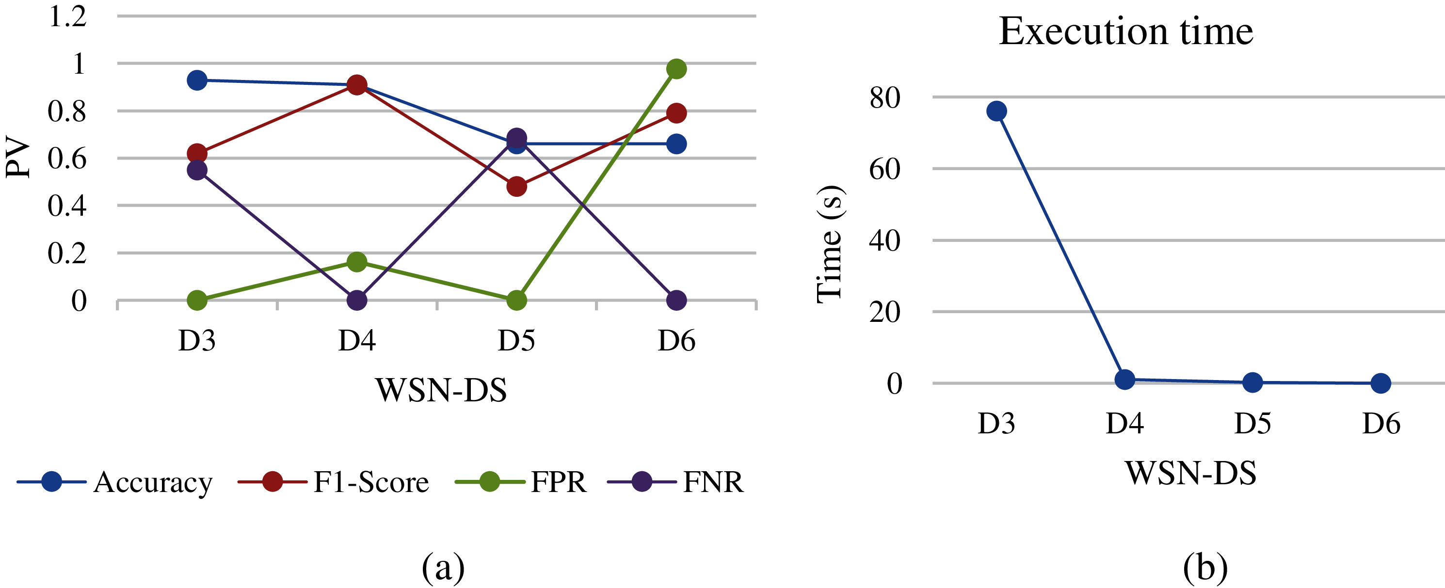
Figure 7: SVM analysis of different WSN-DS dataset sizes: (a) performance metrics, (b) execution time

Figure 8: DT analysis of different WSN-DS dataset sizes: (a) performance metrics, (b) execution time
In KNN, the instance category will be expected based on some instance metrics. The distance measure used in nearest neighbor methods for numerical features can be a simple Euclidean distance. Since WSN-DS is close to this type of feature, the KNN showed good results in accuracy and FPR in all different WSN-DS groups. The highest accuracy was at D3, D4, and D5 which satisfied 100%, and the lowest FPR at all groups was close to 0 as shown in Fig. 5a. However, the FNR showed a gradual decrease through decreasing the data size from D1 to D6. Moreover, F1-Score also showed improvement when the data size decreased from D1 to D6. The execution time also showed that the maximum training time for D1 is 1.8 s and gradually decreased to 0.025 s for D4, which is considered a good result for online use of DoS detection in WSN nodes.
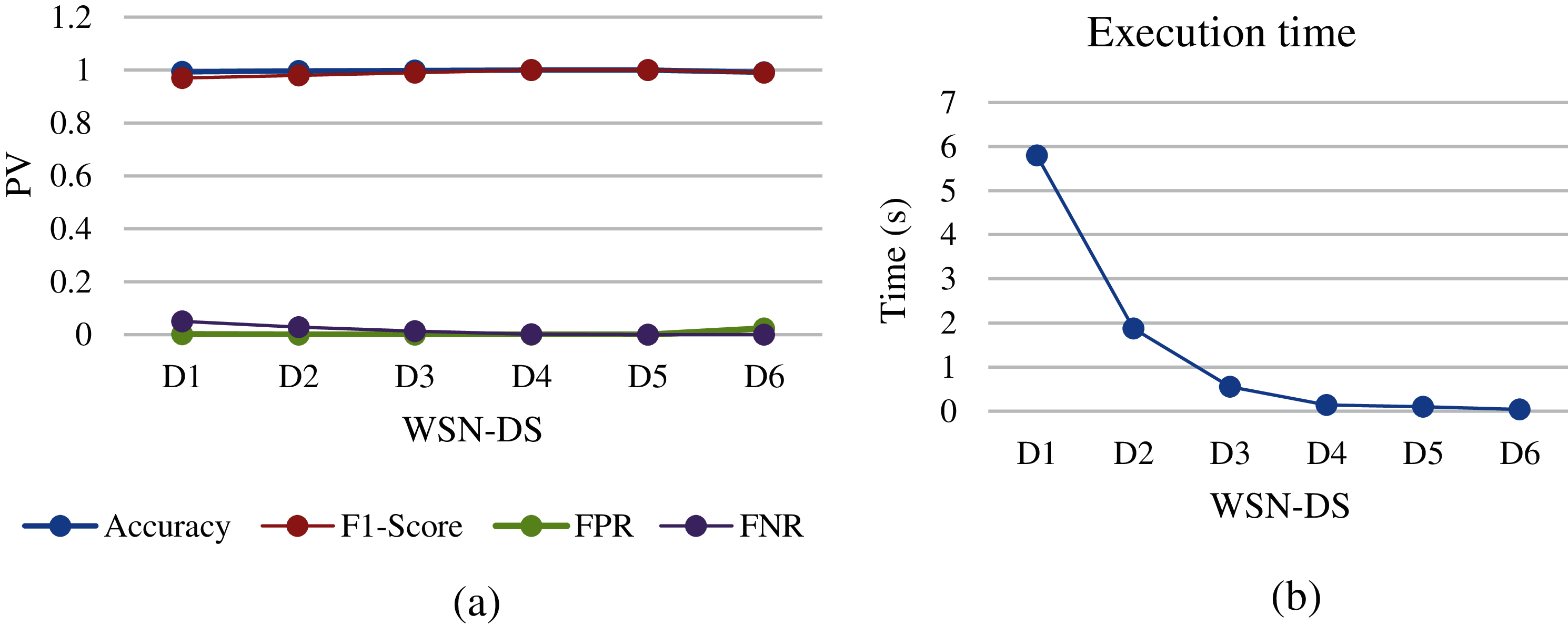
Figure 9: Gboost analysis of different WSN-DS dataset sizes: (a) performance metrics, (b) execution time
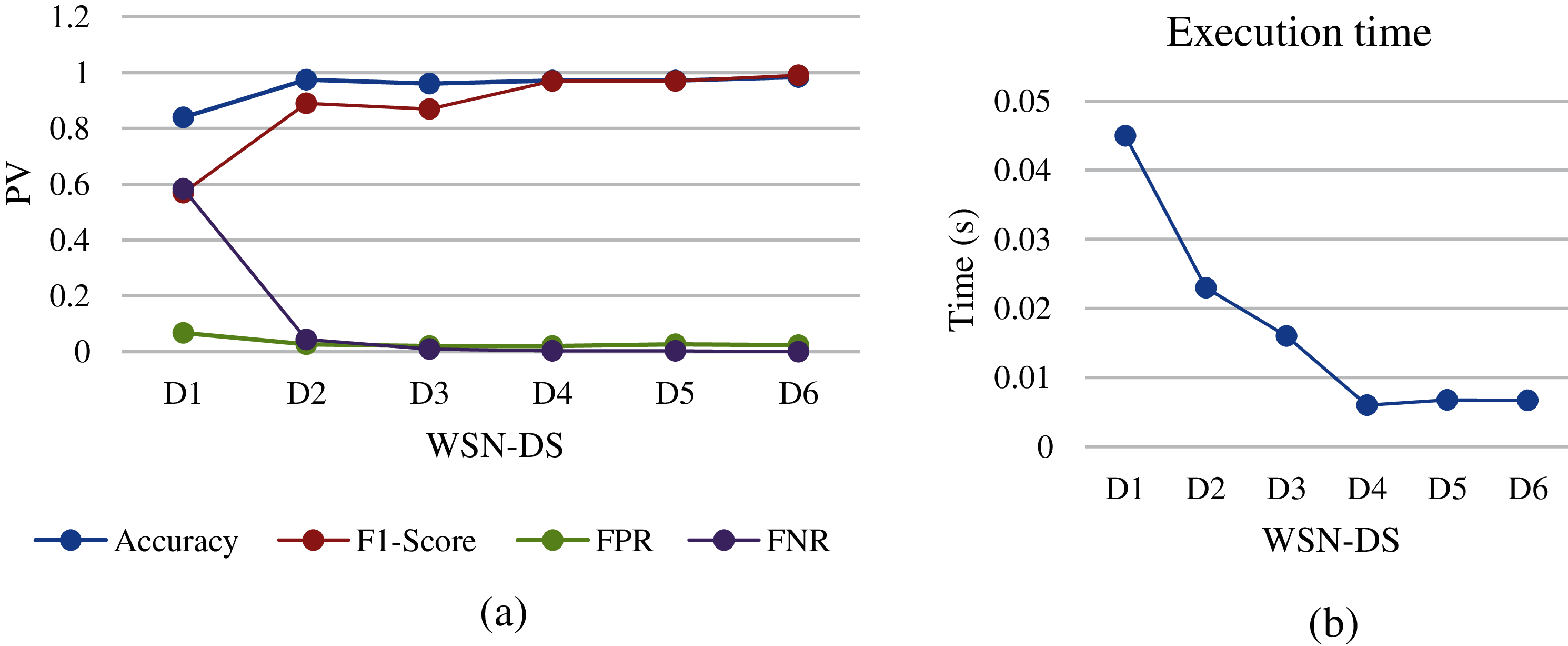
Figure 10: Naïve bayes analysis of different WSN-DS dataset sizes: (a) performance metrics, (b) execution time
LR is widely used in statistical models in many disciplines. It has been used frequently due to its ease of use and accuracy. Since the WSN-DS data relationship is close to linear and there is no missing data between its records, LR showed good results with respect to accuracy, F1-Score, FRP, and FNR as shown in Fig. 6a. Furthermore, the accuracy showed almost no significant changes in the sizing of the WSN-DS groups. This means that LR can be a good choice for inspecting network traffic packets and obtaining high accuracy if the dataset size is small with a linear relationship between them. Furthermore, processing a small amount of dataset reduces the CPU and power consumption of embedded devices. FPR and FNR showed good results in the WSN-DS groups, both of which were close to 0 in the D4 dataset. In addition, the execution time also showed that the maximum training time for D1 is 2.5 s and gradually decreased to 0.25 s for D4, which is consider a good result for online use of DoS detection in WSN nodes.
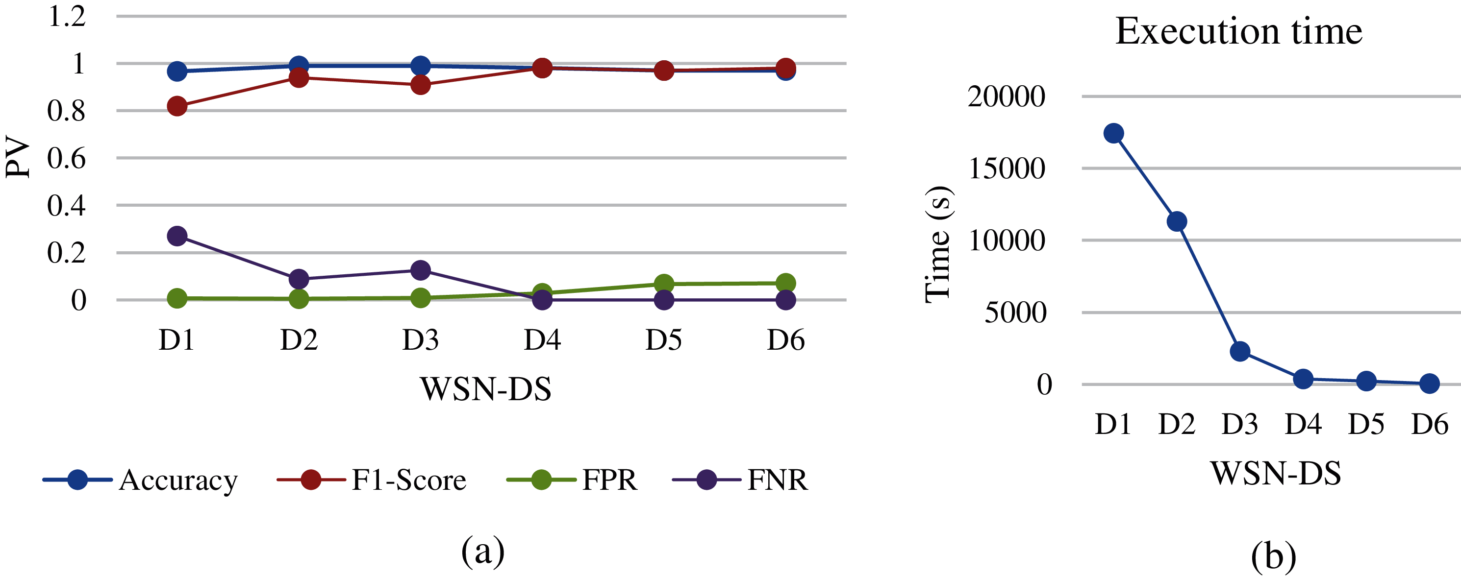
Figure 11: LSTM analysis of different WSN-DS dataset sizes: (a) performance metrics, (b) execution time
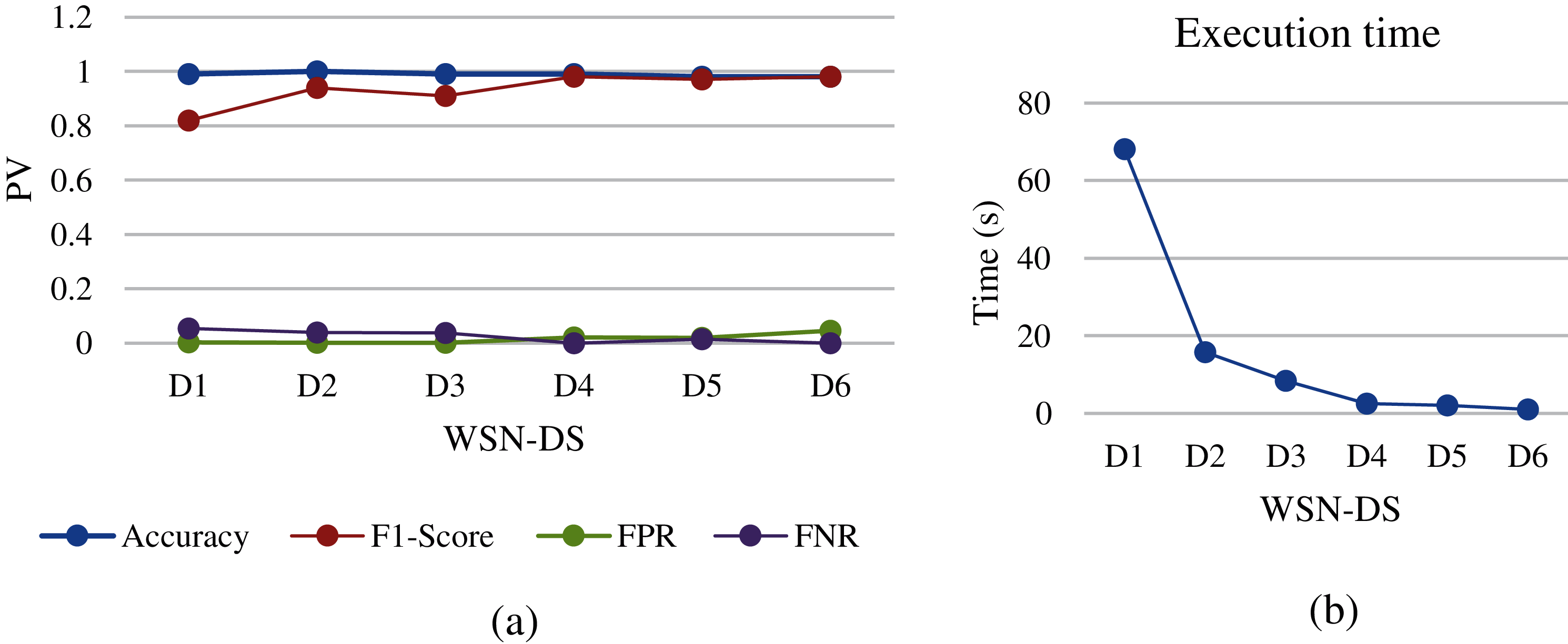
Figure 12: MLP analysis of different WSN-DS dataset sizes: (a) performance metrics, (b) execution time
The idea of SVM is to find the optimal level of separation between two categories by maximizing the margin between the closest points to the categories. However, the SVM has many drawbacks such as high computations for train data, sensitive to noisy data, and unbalanced data sets [18]. Therefore, due to the size of D1 and D2, the SVM was not working and we did not get any results. Moreover, regarding converting all types of attack logs to 0 value, the output will be a binary (0 or 1) and SVM gives better results in a different number of outputs. In addition, the nature of WSN-DS is imbalanced between normal and attack categories. Since the normal range covers more than 89% from all the data, and SVM gives better results when there is a diversity of samples for each category. As results, the SVM came out with poor performance metrics. Accuracy and F-Score showed unstable scores as the WSN-DS was moved from D3 to D6 as shown in Fig. 7a. The highest accuracy achieved at D3 and then started gradually decreases. FPR and FNR also showed random results among the WSN-SD sets and were of high value. In execution time, the algorithm consumed around 80 s to train D3 and then scaled back to close to 0 on the rest of the datasets.
In DT, the attributes of the WSD-DS are determined by the internal nodes, and the branches are the result of each test against each node. Thus, DT structure is simple and fast. In WSN-DS, the DT came out with a good result in accuracy, F1-Score, FPR, and FNR in all datasets as shown in Fig. 8a. The highest accuracy and F1-Score were at D5, and the lowest FNR and FPR were at D5 as well. This means that DT can be a good choice for inspecting network traffic packets and obtaining high accuracy if the dataset size is small with or without a linear relation between them. Therefore, it is considered better than LR for checking network packets. The execution time also showed that the maximum training time for D1 is 9 s and gradually decreases to 0.20 s for D5, which is a good result of using DoS detection online as well.
The Gboost algorithm is an improvement of DT through discovering the unknown relationship between continuous output and dimensional input. The WSN-DS sets showed good results for all performance metrics such as DT. The highest accuracy and F1-Score were at D4 and D5, and the lowest FNR and FPR were at D4 and D5 as shown in Fig. 9a. Moreover, it showed lower execution time compared to DT and this makes it a better choice.
In Naïve Bayes, the fundamental assumption and point in making the prediction is the independence between the attributes of the data set. It is easy to set up and especially useful for large data sets. However, the Naïve Bayes showed good results when the size of WSN-DS decreased from D1 to D6, and the highest accuracy score was at D2 while the F1-Score was not the highest in that group as illustrated in Fig. 10a. Even more surprising is the execution time that algorithm consumes, which is very little compared to similar algorithms. Therefore, it is very good for packets that need direct monitoring with the possibility of obtaining good detection, without paying attention to the volume of data to be analyzed.
Since LSTM is a type of deep learning technique, the process of training and testing will be different from other machine learning algorithms called “shallow”. This type depends on the perceptron layers and weights in order to discover the relationship between interrelated traits. But the most disadvantage of these techniques is the time and power that goes into figuring out these relationships. In general, in terms of inspecting WSN node packets, the time spent on this algorithm was quite large as shown in Fig. 11b. In addition, Fig. 11a showed a slight degradation of accuracy when datasets changed from D1 to D6. Therefore, this algorithm proves that it needs a huge dataset to introduce good performance results. Moreover, The F1-score also shows better results on D4 and D5 compared to other datasets. This is due to the percentage between records labelled by Normal (0) and records labelled by attack (1) in each dataset. The ratio of attack records in datasets D4 and D5 was one-to-two compared to the D1 and D2 as it was 89% (Normal) to 11% (Attack). In addition, the Figure showed the best value for FPR when the dataset is D1 and D2, and its value starts to deteriorate when the dataset changes to D3 and continue, while the FNR starts to improve when the size of dataset becomes smaller, the FNR value has moved from 0.25 in D1 to be 0 in D4. However, the LSTM shows good FNR values compared to other algorithms. Finally, in terms of training execution time, LSTM takes a huge time in the training process, and compared to optimization results, the cost is high for numerical datasets compared to other machine learning algorithms.
Moreover, MLP shown in Fig. 12 results are similar to those of LSTM, with difference in the execution time, which is much less. As for changing datasets, MLP also needs huge data in order to give results with higher accuracy. The F1-score starts to improve while resizing the dataset from D1 to D4, due to the increased percentage of records that are classified as attacked compared to normal records. FPR also showed good performance results while resizing the dataset size from D1 to D3 and starting to increase as the dataset gets smaller and smaller. FNR also showed acceptable performance results. However, the training time for MLP is very low compared to LSTM but compared to other machine learning it is a huge execution time.
In relation to this type of data collected from network traffic, most of its features are numeric statistical values [49]. Therefore, the statistical and logical machine learning techniques will introduce good results in less training time. Therefore, Figs. 5, 8 and 9 show similar chart curve results in all three Figures for most performance metrics (i.e., accuracy, F1-score, FPR and FNR). In addition, the size of a WSN-DS dataset systematically influences the values of these three algorithms’ performance metrics. The accuracy and F1-score start to increase when the dataset changes from D1 to D4, then is nearly constant in size dataset between D4 and D5. After that, the accuracy and F1-score start to decrease after D5 size. Furthermore, the FNR begins decreasing from 0.12 at dataset D1 to 0.001 at D4 and then begins to increase after D5 size. Besides, FPR also shows good results that are close to 0 and being 0 at D4 and D5. However, the Gboost and DT algorithms show the best performance in the results of FNR compared to other machine learning algorithms. Moreover, the same Figs in (5b, 8b, and 9b) show the degradation in training time of machine learning algorithms while reducing the size of the datasets. However, the differences in training times between these three algorithms are a bit close. The KNN shows the lowest training time among them, followed by Gboost and finally DT.
In Figs. 6 and 10, the results of the performance metrics show the improvement when the datasets are D4 and D5 as well. The accuracy and F1-Score show good results at different datasets, but the FRP shows an unstable chart curve with respect to datasets sizes, and it is also higher than Gboost, DT and KNN. Regarding training time, the Naïve bayes in Fig. 10b shows the lowest execution time compared to other machine learning algorithms, while LR in Fig. 6b shows lower execution time compared to DT and Gboost algorithms. In the SVM algorithm, the performance metrics results show unstable accuracy, F1-score, FPR and FNR across all sizes of datasets that were accepted for implementation. The training time for D3 was high compared to other statistical algorithms, it was around 80 s.
Regarding the comparison of machine learning algorithms with each other in different performance metrics models, Figs. 13–17 show these results in each dataset.
Based on Fig. 13, most machine learning algorithms show good performance results in accuracy on different datasets sizes, but the Gboost, DT and KNN are best for numerical network traffic data. The accuracy in the KNN achieved the full score (1) in three datasets, D3, D4, and D5, while the accuracy in both DT and Gboost achieved full score only once in the D5 dataset. Moreover, the same Figure shows a slight similarity in accuracy scores between the MLP and LSTM algorithms related to the sizes of datasets, and also the Fig. 13 shows that the accuracy in MLP has the highest score (1) in the D2 dataset and better than LSTM algorithm. In addition, with respect to the F1-score metric as shown in Fig. 14, Gboost, DT and KNN also introduced the best results in different datasets sizes. The F1-score in the KNN, Gboost, and DT achieved the full score (1) in two datasets, D4, and D5. As previously discussed, the D4 and D5 datasets display the highest F1-score results across all datasets sizes due to the proportions distribution among dependent variable categories.
Moreover, the same Fig. 14 also shows slight similarity in F1-score results between MLP and LSTM algorithms related to sizes of datasets, and also between DT and Gboost, as well as KNN and LR.
Fig. 15 shows the comparison between machine learning algorithms related to FPR, and also the Gboost, KNN, and DT introduced the lowest FPR results. The MLP offered a better FPR compared to LSTM and LR. In FNR as illustrated in Fig. 16, Naïve Bayes introduced the lowest performance results, then the DT and Gboost. However, the SVM offered the worst performance values. Also, the MLP shows good results in FNR compared to LSTM, KNN, and LR.
Finally, in Fig. 17 divide the training execution time into two parts to allow its results to be displayed across all machine learning algorithms. Since the LSTM consumed 17428.7 s compared to Naïve Bayes consumed less than 0.05 s in the D1 dataset. The execution training time consumed in D3 was 2278.67, 76.15, 8.419, 0.818, 0.556, 0.53, 0.515, and 0.016 s in LSTM, SVM, MLP, LR, DT, Gboost, KNN and Naïve Bayes, respectively.

Figure 13: Accuracy comparison between different datasets sizes and machine learning algorithms

Figure 14: F1-Score comparison between different datasets sizes and machine learning algorithms

Figure 15: FPR comparison between different datasets sizes and machine learning algorithms
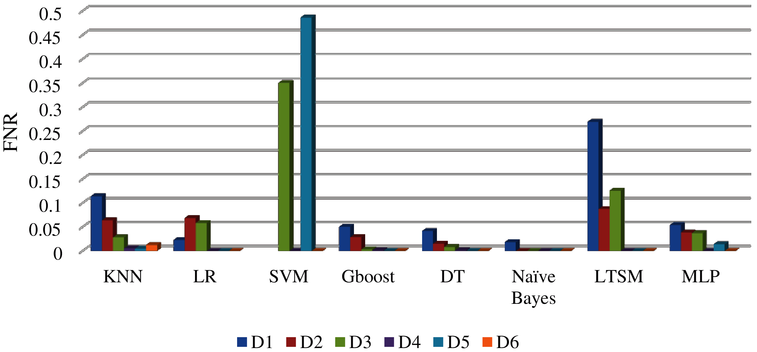
Figure 16: FNR comparison between different datasets sizes and machine learning algorithms

Figure 17: Comparison of training execution time between sizes of different datasets with (a) machine learning algorithms, (b) deep learning algorithms
However, based on this analysis in different machine learning algorithms using different WSN datasets, we conclude that the numerical analysis of DoS in wireless sensor networks traffic does not require complex deep learning algorithms to detect the attack packets. Moreover, a dataset containing between 3000 to 6000 records is sufficient to carry out the training process and obtain a high-performance prediction, if the percentage of data between the labelled categories is sufficient to differentiate these categories. In D4 and D5, the percentage between two labels (dependent variable) are two-to-one, while in D1 it was from 88% to 11% (normal to attack).
In the next section, we will choose the Gboost algorithm to implement in WSN network simulation. We select it based on the highest performance in accuracy, F1-score, FPR, and FNR in all datasets and specially on D4 and D5. Moreover, it has an acceptable training execution time in D4 and D5 which ranges from 0.14 s in D4 to 0.094 s in D5.
To implement this algorithm in WSN networks simulation, we need to find out the Gboost output model from the training process. Therefore, as the dependent variable of the WSN-DS dataset has two values (0 “Normal” or 1 “Attack”), the probability (P) represents the relationship between the independent variables and dependent variables. Eq. (5) represents this probability [42]:
where n is the number of WSN-DS dataset features, x is the WSN-DS feature, β0 is an intercept, and β1, β2, βnare the regression coefficients for WSN-DS features. In addition, from the training process of Gboost algorithm the regression coefficient values come out and the Gboost prediction is ready for testing. The regression coefficient values for the Gboost are illustrated in Tab. 5. Moreover, the Is_CH, Join_Req Received, Send_code, ADV_R, and ADV_S messages are among the most important features related to the Gboost-DoS detection process.

The probability of y from xn is calculated in Eq. (6).
where y is a dependent variable (Label).
5.2 Complexity Analysis for the WSN Networks Lifetime on Gboost Approach
In this section, we will analyse the impact of DoS detection by using the Gboost algorithm on WSN network lifetime. The lifetime of the network is calculated when the power of some WSN nodes reaches 0.
In the simulation environment, Contiki operating systems with Cooja simulator are used to simulate WSN network architecture [51]. The modified 6LoWPAN protocol will be used as discussed in [25] to manage and control the WSN node's hardware and software. The simulation is running on the same machine that was discussed in 5.1.1. The default parameters used in the wireless networks architecture are plotted in Tab. 6, and some parameters values in the table are taken from the values in [25].

For the DoS detection evaluation using the ‘Gboost scheme’, we will simulate the first scenario regarding reference parameters, encryption, and authentication processes, and then extract the network lifetime. In the second scenario, we will add a Gboost-DoS detection mechanism to the first scenario and run it to see the effect of monitoring and packet inspection in each CH to the network lifetime. The Gboost-DoS output model is distributed to all WSN nodes and each WSN node becomes a CH, it will start monitoring ordinary WSN node activities associated with it in second and third WSN node layers, then find data features and calculate y for each node. For each positive y, the CH will create a counter table for the WSN node that received suspicious packets, and calculate from one to α, if counter reaches this value in period of time (t), the CH will block this node and send broadcast message to other CHs and AP for this case. Moreover, these counter tables are forwarded between CH nodes so that all of them are aware of these numbers, since the work environment is mobile and the WSN nodes can navigate and share another CH. However, the idea of a counter table is important and is to reduce the FNR in WSN networks.
In the simulation, the WSN nodes are initially spread with dimensions of 500 × 500 terrain associated with nine CHs at the initial values as seen in Fig. 18. Next, the WSN nodes continue to travel in a random direction at a rate of 5 meters per second. The initial energy of the WSN node to 1.5 Joule and the simulation time set to 500 s to allow some of the WSN node's energy in the first scenario to reach 0.
Moreover, each ordinary node sends 64 packets per second to its CH node and each packet size is 1000 bits. If the node is CH, the received packets will be forwarded to the neighbour CH. Moreover, the monitoring of nodes packets activity occur in constant time interval, and the statistical calculation for each DoS attack during these time intervals (t) will be the same data features calculation of [23]. regarding to Gboost DoS detection model, we suppose that the energy consumption per each packet inspection will be 0.001 J, and depends on this energy consumption value the analysis effect of the Gboost DoS detection on the WSN network lifetime is illustrated on Fig. 19.

Figure 18: Simulation WSN nodes
As illustrated from Fig. 19, the increment of initial power in WSN nodes increases the lifetime of WSN networks in both scenarios. This resemblance is due to the positive relationship between WSN node initial power and the duration time. Moreover, from the same Fig. 19, we observe that the variation of the network lifetime between two scenarios increases with the increases in the initial power of the WSN nodes. This variation increases from 35% to 59% when the WSN node initial power increases from 0.75 to 1.5 J. The reason for the increase in this variance is due to the increase in the rate of packets received by the CH nodes, which in turn will lead to an increase in the rate of the inspection and verification messages. This in turn also leads to an increase in the rate of power consumption within the CH nodes, and thus the result is a decrease in the lifetime of networks. The results show the Gboost-detection algorithm decreases the network lifetime by 35%, 40%, 43%, and 59% compared to the Gboost-free scenario, respectively.

Figure 19: Analysis the effect of Gboost algorithm on WSN network lifetime
In this paper, we have analysed the performance of various machine learning algorithms belonging to different classification categories (Statistical-based, Logic-based, Instance-Based, and Deep Learning-based) on WSN-DS datasets to help detect DoS attacks. These machine learning algorithms were KNN, LR, SVM, DT, Naïve Bayes, LSTM, and MLP. Moreover, the WSN-SD was divided into different datasets to analyse the performance of these algorithms on each dataset size. Furthermore, one of these algorithms was selected to analyse its functions on the lifetime of the WSN network. Python 3.8 within Jumyter Network software has been used to obtain the accuracy, F1-score, FPR, FNR, and training execution time for each algorithm. Cooja simulator have also been used to obtain the WSN network lifetime and the simulation environment was managed by the clustering management algorithm which was supposed in modern references.
The performance analysis results of the machine learning algorithms in WSN-SD show that the dataset that collected from WSN network traffic are numeric statistical values. Therefore, the statistical and logical classification algorithms have the best performance metrics, and Gboost was the best based on the overall average of performance metrics in different WSN-DS datasets. Moreover, a dataset containing between 3000 to 6000 records is sufficient to carry out the training process and obtain a high-performance prediction, if the percentage of data between the labelled categories is sufficient to differentiate these categories.
The Gboost improved the average of accuracy across all WSN datasets by 0.29%, 2%, 26%, 5%, 2%, and 0.8% compared to KNN, LR, SVM, Naïve Bayes, LSTM, and MLP, respectively. In DT accuracy, it was very close to Gboost. In an average of F1-score, Gboost improved it by 2%, 5%, 41%, 12%, 58%, and 58% compared to KNN, LR, SVM, Naïve Bayes, LSTM, and MLP, respectively. Also DT in F1-score showed the similar result to Gboost. Furthermore, the Gboost reduced the average FPR in all WSD-DS datasets by 87%, 97%, 27%, 89%, 86%, and 72% compared to LR, SVM, DT, Naïve Bayes, LSTM, and MLP. The KNN showed a 36% better reduction compared to Gboost. In average FNR, the Gboost reduced it by 63%, 43%, 93%, 82%, and 41% compared to KNN, LR, SVM, LSTM, and MLP, respectively. FNR in DT and Naïve Bayes was 26% and 350% lower than Gboost. Finally, on average training execution time, Gboost used less time compared to DT, SVD, LSTM, MLP at 32%, 927%, 9997%, and 913% respectively. Moreover, the KNN, LR, Naïve Bayes used less average training execution time by 128%, 74%, and 808% compared to Gboost, respectively. In network lifetime, the Gboost reduced it by 32% compared to standard scenario.
In the future research, we intend to collect new WSN network dataset from 6LoWPAN protocol and add new features related to packet drop per flow, packet size per flow, flow change ratio, and packet change ratio. Moreover, we can use the cumulative difference of correctly classified states computed by the custom sniffer to generate a more solid conclusion regarding the node state. Furthermore, to employ or suppose a lightweight mechanism determines the most important features of datasets. The best features are selected before the training stage to improve the performance machine learning algorithms output. Additionally, we need to examine the effect of percentage size of each class in dependent variables on the performance of machine learning algorithms.
Funding Statement: The authors received no specific funding for this study.
Conflicts of Interest: The authors declare that they have no conflicts of interest to report regarding the present study.
1. M. Al-Emran, S. I. Malik and M. N. Al-Kabi, “A Survey of internet of things (IoT) in education: Opportunities and challenges,” in Studies in Computational Intelligence, vol. 846, Springer International Publishing, pp. 197–209, 2020. [Google Scholar]
2. G. Zhang, L. Kou, L. Zhang, C. Liu, Q. Da et al., “A new digital watermarking method for data integrity protection in the perception layer of IoT,” Security and Communication Networks, vol. 2017, pp. 1–12, 2017. [Google Scholar]
3. L. Yi, X. Tong, Z. Wang, M. Zhang, H. Zhu et al., “A novel block encryption algorithm based on chaotic s-box for wireless sensor network,” IEEE Access, vol. 7, pp. 53079–53090, 2019. [Google Scholar]
4. H. Al-Kashoash, H. Kharrufa, Y. Al-Nidawi and A. H. Kemp, “Congestion control in wireless sensor and 6LoWPAN networks: Toward the internet of things,” Wireless Networks, vol. 25, no. 8, pp. 4493–4522, 2019. [Google Scholar]
5. X. Zhang, H. M. Heys and C. Li, “Energy efficiency of encryption schemes applied to wireless sensor networks,” Security and Communication Networks, vol. 5, no. 7, pp. 789–808, 2012. [Google Scholar]
6. Y. Yang, L. Wu, G. Yin, L. Li and H. Zhao, “A survey on security and privacy issues in internet-of-things,” IEEE Internet of Things Journal, vol. 4, no. 5, pp. 1250–1258, 2017. [Google Scholar]
7. G. Glissa and A. Meddeb, “6LoWPAN Multi-layered security protocol based on IEEE 802.15.4 security features,” in 2017 13th Int. Wireless Communications and Mobile Computing Conf., Valencia, Spain, pp. 264–269, 2017. [Google Scholar]
8. C.-C. Lee, “Security and privacy in wireless sensor networks: Advances and challenges,” Sensors, vol. 20, no. 3, pp. 744, 2020. [Google Scholar]
9. T. Kaur, K. K. Saluja and A. K. Sharma, “DDOS attack in WSN: A survey,” in 2016 Int. Conf. on Recent Advances and Innovations in Engineering, Jaipur, Rajasthan, India, pp. 23–27, 2016. [Google Scholar]
10. M. N. U. Islam, A. Fahmin, M. S. Hossain and M. Atiquzzaman, “Denial-of-service attacks on wireless sensor network and defense techniques,” Wireless Personal Communications, vol. 116, pp. 1993–2021, 2020. [Google Scholar]
11. K. Khan, A. Mehmood, S. Khan, M. A. Khan, Z. Iqbal et al., “A survey on intrusion detection and prevention in wireless ad-hoc networks,” Journal of Systems Architecture, vol. 105, no. September 2019, pp. 101701, 2020. [Google Scholar]
12. D. Praveen Kumar, T. Amgoth and C. S. R. Annavarapu, “Machine learning algorithms for wireless sensor networks: A survey,” Information Fusion, vol. 49, pp. 1–25, 2019. [Google Scholar]
13. F. Cauteruccio, L. Cinelli, E. Corradini, G. Terracina, D. Ursino et al., “A framework for anomaly detection and classification in multiple IoT scenarios,” Future Generation Computer Systems, vol. 114, pp. 322–335, 2021. [Google Scholar]
14. J. Cheng, J. Zhou, Q. Liu, X. Tang and Y. Guo, “A DDoS detection method for socially aware networking based on forecasting fusion feature sequence,” Computer Journal, vol. 61, no. 7, pp. 959–970, 2018. [Google Scholar]
15. R. Vishwakarma and A. K. Jain, “A survey of DDoS attacking techniques and defence mechanisms in the IoT network,” Telecommunication Systems, vol. 73, no. 1, pp. 3–25, 2020. [Google Scholar]
16. S. Otoum, B. Kantarci and H. T. Mouftah, “On the feasibility of deep learning in sensor network intrusion detection,” IEEE Networking Letters, vol. 1, no. 2, pp. 68–71, 2019. [Google Scholar]
17. D. Wu, Z. Jiang, X. Xie, X. Wei, W. Yu et al., “LSTM learning with Bayesian and Gaussian processing for anomaly detection in industrial IoT,” IEEE Transactions on Industrial Informatics, vol. 16, no. 8, pp. 5244–5253, 2020. [Google Scholar]
18. W. Zhang, D. Han, K. C. Li and F. I. Massetto, “Wireless sensor network intrusion detection system based on MK-eLM,” Soft Computing, vol. 24, no. 16, pp. 12361–12374, 2020. [Google Scholar]
19. A. P. Abidoye and I. C. Obagbuwa, “DDos attacks in WSNs: Detection and countermeasures,” IET Wireless Sensor Systems, vol. 8, no. 2, pp. 52–59, 2018. [Google Scholar]
20. R. F. Bikmukhamedov and A. F. Nadeev, “Lightweight machine learning classifiers of IoT traffic flows,” 2019 Systems of Signal Synchronization, Generating and Processing in Telecommunications, Yaroslavl, Russia, 2019. [Google Scholar]
21. A. Depari, P. Ferrari, A. Flammini, S. Rinaldi and E. Sisinni, “Lightweight machine learning-based approach for supervision of fitness workout,” SAS 2019-2019 IEEE Sensors Applications Symp., Conf. Proceedings, Sophia Antipolis, France, 2019. [Google Scholar]
22. M. Premkumar and T. V. P. Sundararajan, “DLDM: Deep learning-based defense mechanism for denial of service attacks in wireless sensor networks,” Microprocessors and Microsystems, vol. 79, pp. 103278, 2020. [Google Scholar]
23. I. Almomani, B. Al-Kasasbeh and M. Al-Akhras, “WSN-Ds: A dataset for intrusion detection systems in wireless sensor networks,” Journal of Sensors, vol. 2016, pp. 41525–41550, 2016. [Google Scholar]
24. Y. Chen and S. Li, “A lightweight anomaly detection method based on svdd for wireless sensor networks,” Wireless Personal Communications, vol. 105, no. 4, pp. 1235–1256, 2019. [Google Scholar]
25. O. A. Khashan, R. Ahmad and N. M. Khafajah, “An automated lightweight encryption scheme for secure and energy-efficient communication in wireless sensor networks,” Ad Hoc Networks, vol. 115, pp. 102448, 2021. [Google Scholar]
26. V. Kumar and S. Tiwari, “Routing in IPv6 over low-power wireless personal area networks (6LoWPANA survey,” Journal of Computer Networks and Communications, vol. 2012, pp. 316839, 2012. [Google Scholar]
27. M. Bouaziz and A. Rachedi, “A survey on mobility management protocols in wireless sensor networks based on 6LoWPAN technology,” Computer Communications, vol. 74, pp. 3–15, 2016. [Google Scholar]
28. P. M. Kumar and U. D. Gandhi, “Enhanced DTLS with CoAP-based authentication scheme for the internet of things in healthcare application,” Journal of Supercomputing, vol. 76, no. 6, pp. 3963–3983, 2020. [Google Scholar]
29. O. Can and O. K. Sahingoz, “A survey of intrusion detection systems in wireless sensor networks,” in 2015 6th Int. Conf. on Modeling, Simulation, and Applied Optimization (ICMSAOIstanbul, Turkey, pp. 1–6, 2015. [Google Scholar]
30. R. Vangipuram, R. K. Gunupudi, V. K. Puligadda and J. Vinjamuri, “A machine learning approach for imputation and anomaly detection in IoT environment,” Expert Systems, vol. 37, no. 5, pp. 1–16, 2020. [Google Scholar]
31. B. Ahmad, W. Jian, Z. A. Ali, S. Tanvir and M. S. A. Khan, “Hybrid anomaly detection by using clustering for wireless sensor network,” Wireless Personal Communications, vol. 106, no. 4, pp. 1841–1853, 2019. [Google Scholar]
32. M. Yamauchi, Y. Ohsita, M. Murata, K. Ueda and Y. Kato, “Anomaly detection in smart home operation from user behaviors and home conditions,” IEEE Transactions on Consumer Electronics, vol. 66, no. 2, pp. 183–192, 2020. [Google Scholar]
33. K. J. Singh and T. De, “MLP-Ga based algorithm to detect application layer DDoS attack,” Journal of Information Security and Applications, vol. 36, pp. 145–153, 2017. [Google Scholar]
34. G. M. Borkar, L. H. Patil, D. Dalgade and A. Hutke, “A novel clustering approach and adaptive SVM classifier for intrusion detection in WSN: A data mining concept,” Sustainable Computing: Informatics and Systems, vol. 23, pp. 120–135, 2019. [Google Scholar]
35. J.-W. Ho, M. Wright and S. K. Das, “Distributed detection of mobile malicious node attacks in wireless sensor networks,” Ad Hoc Networks, vol. 10, no. 3, pp. 512–523, 2012. [Google Scholar]
36. P. Ballarini, L. Mokdad and Q. Monnet, “Modeling tools for detecting DoS attacks in WSNs,” Security and Communication Networks, vol. 6, no. 4, pp. 420–436, 2013. [Google Scholar]
37. C. Ioannou and V. Vassiliou, “An intrusion detection system for constrained wsn and iot nodes based on binary logistic regression,” in Proc. of the 21st ACM Int. Conf. on Modeling, Analysis and Simulation of Wireless and Mobile Systems, New York, NY, USA, pp. 259–263, 2018. [Google Scholar]
38. O. Osanaiye, A. S. Alfa and G. P. Hancke, “A statistical approach to detect jamming attacks in wireless sensor networks,” Sensors, vol. 18, no. 6, pp. 1691, 2018. [Google Scholar]
39. H. Qu, L. Lei, X. Tang and P. Wang, “A lightweight intrusion detection method based on fuzzy clustering algorithm for wireless sensor networks,” Advances in Fuzzy Systems, vol. 2018, pp. 4071851, 2018. [Google Scholar]
40. L. Coppolino, S. DAntonio, A. Garofalo and L. Romano, “Applying data mining techniques to intrusion detection in wireless sensor networks,” in 2013 Eighth Int. Conf. on P2P, Parallel, Grid, Cloud and Internet Computing, Compiegne, France, pp. 247–254, 2013. [Google Scholar]
41. A. Garofalo, C. Di Sarno and V. Formicola, “Enhancing intrusion detection in wireless sensor networks through decision trees,” In: Vieira, M., Cunha, J. C. (Eds.Dependable Computing, Berlin, Heidelberg: Springer Berlin Heidelberg, pp. 1–15, 2013. [Google Scholar]
42. A. Hameed and A. Leivadeas, “Iot traffic multi-classification using network and statistical features in a smart environment,” in 2020 IEEE 25th Int. Workshop on Computer Aided Modeling and Design of Communication Links and Networks (CAMAD), vol. 2020, pp. 1–7, 2020. [Google Scholar]
43. W. Li, P. Yi, Y. Wu, L. Pan and J. Li, “A new intrusion detection system based on knn classification algorithm in wireless sensor network,” Journal of Electrical and Computer Engineering, vol. 2014, pp. 1–8, 2014. [Google Scholar]
44. X. Lu, D. Han, L. Duan and Q. Tian, “Intrusion detection of wireless sensor networks based on IPSO algorithm and BP neural network,” International Journal of Computational Science and Engineering, vol. 22, no. 2–3, pp. 221–232, 2020. [Google Scholar]
45. S. Sujanthi and S. Nithya Kalyani, “SecDL: QoS-aware secure deep learning approach for dynamic cluster-based routing in WSN assisted IoT,” Wireless Personal Communications, vol. 114, no. 3, pp. 2135–2169, 2020. [Google Scholar]
46. K. A. Darabkh, M. Z. El-Yabroudi and A. H. El-Mousa, “BPA-Crp: A balanced power-aware clustering and routing protocol for wireless sensor networks,” Ad Hoc Networks, vol. 82, pp. 155–171, 2019. [Google Scholar]
47. R. Ahmad, M. Ismail, E. A. Sundararajan, N. E. Othman and A. M. Zain, “Performance of movement direction distance-based vertical handover algorithm under various femtocell distributions in HetNet,” in 2017 IEEE 13th Malaysia Int. Conf. on Communications, MICC 2017, vol. 2017-November, no. Micc, Jahor, Malaysia, pp. 253–258, 2018. [Google Scholar]
48. I. Sharafaldin, A. H. Lashkari, S. Hakak and A. A. Ghorbani, “Developing realistic distributed denial of service (DDoS) attack dataset and taxonomy,” in 2019 Int. Carnahan Conf. on Security Technology, vol. 2019-Octob, no. Cic, pp. 1–8, 2019. [Google Scholar]
49. N. Koroniotis, N. Moustafa, E. Sitnikova and B. Turnbull, “Towards the development of realistic botnet dataset in the internet of things for network forensic analytics: Bot-IoT dataset,” arXiv.org, vol. 100, pp. 779–796, 2018. [Google Scholar]
50. Jupyter. [Online]. Available: https://jupyter.org/ (accessed on May 26, 2021). [Google Scholar]
51. Y. Bin Zikria, M. K. Afzal, F. Ishmanov, S. W. Kim and H. Yu, “A survey on routing protocols supported by the contiki internet of things operating system,” Future Generation Computer Systems, vol. 82, pp. 200–219, 2018. [Google Scholar]
 | This work is licensed under a Creative Commons Attribution 4.0 International License, which permits unrestricted use, distribution, and reproduction in any medium, provided the original work is properly cited. |