Computers, Materials & Continua DOI:10.32604/cmc.2022.019630
Article

Predicting Resource Availability in Local Mobile Crowd Computing Using Convolutional GRU

Pijush Kanti Dutta Pramanik1, Nilanjan Sinhababu2, Anand Nayyar3,4,*, Mehedi Masud5 and Prasenjit Choudhury1

1Department of Computer Science & Engineering, National Institute of Technology, Durgapur, India
2Reliability Engineering Centre, Indian Institute of Technology Kharagpur, India
3Graduate School, Duy Tan University, Da Nang, 550000, Vietnam
4Faculty of Information Technology, Duy Tan University, Da Nang, 550000, Vietnam
5Department of Computer Science, College of Computers and Information Technology, Taif University, Taif, 21944, Saudi Arabia
*Corresponding Author: Anand Nayyar. Email: anandnayyar@duytan.edu.vn
Received: 19 April 2021; Accepted: 20 May 2021

Abstract: In mobile crowd computing (MCC), people’s smart mobile devices (SMDs) are utilized as computing resources. Considering the ever-growing computing capabilities of today’s SMDs, a collection of them can offer significantly high-performance computing services. In a local MCC, the SMDs are typically connected to a local Wi-Fi network. Organizations and institutions can leverage the SMDs available within the campus to form local MCCs to cater to their computing needs without any financial and operational burden. Though it offers an economical and sustainable computing solution, users’ mobility poses a serious issue in the QoS of MCC. To address this, before submitting a job to an SMD, we suggest estimating that particular SMD’s availability in the network until the job is finished. For this, we propose a convolutional GRU-based prediction model to assess how long an SMD is likely to be available in the network from any given point of time. For experimental purposes, we collected real users’ mobility data (in-time and out-time) with respect to a Wi-Fi access point. To build the prediction model, we presented a novel feature extraction method to be applied to the time-series data. The experimental results prove that the proposed convolutional GRU model outperforms the conventional GRU model.

Keywords: Resource selection; resource availability; mobile grid; mobile cloud; ad-hoc cloud; crowd computing; deep learning; GRU; CNN; RNN

1  Introduction

The continuous growth of IT (information technology) infrastructure has led to severe environmental concerns [1]. Utilizing existing computing devices to their fullest is a sustainable option. In this regard, mobile crowd computing (MCC) has been considered a suitable economical solution for sustainable computing [2]. In MCC, the public’s (crowd’s) mobile devices are exploited as computing resources. Today’s smart mobile devices (SMDs) (smartphones and tablets) are loaded with impressive hardware along with good battery life and flexible charging options; as a result, MCC has become a potential solution for affordable and flexible HPC [3,4]. In this computing paradigm, the computing tasks are sent by a coordinator to the connected and pre-agreed SMDs. The tasks are executed on the SMDs opportunistically, and the results are sent back to the coordinator.

Since in MCC, the computing resources (contributing SMDs) are mobile, there is no guarantee of their availability in a local MCC, where the devices are connected to a local network (typically Wi-Fi access point) for contributing their resources to an organizational crowd computing application. This uncertainty affects the QoS (quality of service) of MCC significantly because if an SMD leaves the network before completing the assigned job, it has to be reassigned to another SMD, which introduces a significant delay or, in the worst case, would result in job loss [5].

To address this issue, we suggest, before a job is submitted to an SMD, it is to be estimated if that particular SMD would be available for the duration required to complete the job. If the SMD’s availability duration is greater than the job execution time, only then the job would be scheduled to that particular SMD. In a local MCC model, generally, most SMDs connect to an access point one or more times a day and stay for a certain duration in every session. Therefore, it is possible to find a pattern of their incoming and outgoing timings and, correspondingly, their availability in the network. Based on this information, the chances of each SMD being available up to a specific duration from any given point of time can be predicted. Using this knowledge before scheduling a job to an SMD will allow avoiding unnecessary job loss or job handovers.

General machine learning based prediction models cannot provide satisfactory prediction accuracy in cases where the data context changes frequently. The user mobility data change with respect to the users’ behavior in a long duration. This change needs to be captured by the prediction models to provide expected prediction results. To capture this long-term user mobility behavior, we are required to use deep learning based model like RNN (recurrent neural networks), which is capable of retaining long-term contextual information due to the presence of specialized memory.

For predicting SMDs’ availability, we adopted a GRU (gated recurring units) based model. GRU, a gating mechanism from the RNN family, was introduced by Cho et al. [6] in 2014 and has been popularly used in sequence modeling and time-series predictions. The reason behind preferring GRU over LSTM (long-short term memory), another approach popularly used for time-series analysis and predictions, is that GRUs are more straightforward and easier to modify. Also, since GRU uses fewer training parameters, it needs much less memory, the GRU-based models are faster to train and execute than LSTM models [7]. GRUs are generally preferred when we require a decent degree of accuracy but do not have sufficient computing resources to train data samples with longer sequences.

However, using only the prediction model without proper feature extraction does not guarantee achieving the expected prediction accuracy. The feature extraction helps in improving the model performance by capturing the most relevant features from the data. The known feature extraction methods generally can extract the required features for a particular task. But this is not applicable in every case because usually, we do not have prior knowledge of the most dominating features. Therefore, we needed to frame a dynamic feature extraction methodology for solving the proposed resource availability prediction problem. For this, we used convolutional feature extraction followed by the GRU prediction model.

The followings are the significant contributions of this paper:

•   Based on the historical in-time and out-time of SMDs with respect to a Wi-Fi access point, a prediction model is presented to predict each SMD’s availability at any given point of time.

•   A novel convolutional feature extraction and GRU-based prediction method, named CGRU (convolutional GRU), are presented.

•   The performance of the proposed CGRU is compared with the traditional GRU-based prediction, showing the superiority of CGRU in predicting time-series data.

The rest of the paper is organized as follows. Section 2 discusses the related work. Section 3 discusses the SMD availability prediction method’s details, including data collection and preparation, feature optimization, and prediction modeling. The test results are analyzed in Section 4. The paper is concluded in Section 5.

2  Related Work

Sipos et al. [8] proposed a method to estimate mobile devices’ availability where these devices were used to form a distributed storage system in a P2P (peer-to-peer) fashion. The node mobility scenario was simulated, and three classifiers (logistic regression, naive Bayes, and alternating decision tree) were used to check the accuracy of the prediction model. The prediction is based on the declaration by the nodes for their availability or unavailability for the next considered time period.

To have a better QoS of a P2P mobile cloud, Pramanik et al. [9] proposed a mobility prediction method to find the probability that a group of SMD users would be in a close vicinity over a period of time. They estimated the relative stability of the SMD users based on their short-term (two hours) as well as long-term (78 days) mobility patterns.

Vaithiya et al. [10] attempted to predict mobile resources’ availability for task scheduling algorithms in a mobile grid. To address the node mobility issue in an ad-hoc mobile grid, Selvi et al. [11] profiled the mobile users’ regular movements over time. But both of these works did not consider the historical characteristics of mobile devices.

Farooq et al. [12] proposed a mobility model where the previous records of the contact duration of two devices were used to predict the duration a resource-providing node may remain in the vicinity of the resource requesting node in a mobile grid. Based on the predicted time, the task assignment decision is taken. Here the contact is calculated based on their GPS locations.

Habak et al. [13] introduced mobile devices’ presence time prediction in their proposed mobile device cloud control system. Here, each mobile node is supposed to inform about its probable departure time for each session to the controller node in prior. However, it may not always hold true because the nodes may leave the network before the declared departure time, intentionally or unintentionally.

Zhou et al. [14] proposed a stability-aware mobile device selection method in a mobile cloud environment. They designed a model to store the movement history of each mobile device.

RNNs are popularly being used in predicting time-series data. In time-series data, the previous information or state of the data is necessary for prediction, which can be done using RNN. Regular RNNs suffer from the exploding and vanishing gradient problems, which are not present in GRU. It encouraged researchers to use GRU in time-series analysis and prediction problems on various application areas [15,16,17,18].

However, we could not find any research work that uses deep-learning based model to predict resource availability by analyzing user mobility patterns in a crowd computing system. In our recent work [19], to address the same problem, we used the ConvLSTM module that is readily available in Keras1 Python API. The model achieved an average accuracy of 78.43%. Since we did not have much flexibility in manipulating the model, we were limited in improving the model performance. This led us to work on this proposed paper, where we had much flexibility in feature optimization and model tuning.

3  SMD Availability Prediction

In this section, we present the necessary tasks carried out for framing and implementing the prediction model for SMD availability.

3.1 System Assumptions

In our local MCC, we assume that the SMDs get connected to a WLAN through a Wi-Fi access point. The owners of the SMDs may come within the range of the network and get connected more than once a day. Most of the time, they follow a repetitive pattern. A local central coordinator of the MCC system has knowledge of the hardware and software specifications of the connected SMDs. Before assigning the crowd computing tasks to the SMDs, the coordinator maintains a ranked list of the SMDs. The ranking is done based on the computing resources of the SMDs. The SMDs are selected for task allocation from the top of the ranked list. However, before dispatching the task to an SMD, an added checking is done. It is checked if the to-be-assigned SMD will be available in the network till the job is completed. Based on the past mobility history, if it is predicted that the considered SMD will probably be available until the task completion, then only the task will be dispatched to that particular SMD. Otherwise, the next SMD in the list will be considered, and again the availability of this SMD will be checked. This will continue until the suitable SMD of which the availability period is greater than the task execution time is found. A general flow diagram for our SMD selection approach is shown in Fig. 1.

Figure 1: A general flow diagram for SMD selection

3.2 Data Collection

We collected user data traces from the Wi-Fi access point deployed at the Data Engineering Lab of the Department of Computer Science & Engineering at National Institute of Technology, Durgapur. The lab is generally accessed by the institute’s research scholars, the project students, faculty members, and the technical staff. For every entry of an SMD to the network, the in-time and out-time are noted. The schema of the log database (MySQL) is shown in Fig. 2.

Figure 2: The database schema for SMD availability logging

We developed a logger program using Python 3.6 for gathering the data. The Python script constantly monitors the wireless network interfaces. MAC addresses were used to identify the devices (UID) connected to the access point. Since we wanted to consider only SMDs, we avoided logging for other connected devices than SMDs (e.g., PCs and laptops).

We ran the data logging program for eight months and collected the user data during this period. We chose the data of those 150 days (Td) when there was the maximum concentration of the connected devices from the collected data. From this 150-day data, we further created a sub dataset containing user data of 120 days. We tested the model on two different volumes of datasets to understand the model’s effectiveness with different types of crowd computing applications.

3.3 Data Preparation

Before feeding the time-series data into the GRU model, we needed to prepare the data that would be suitable for applying convolutional filters for feature extraction. The user mobility data are time-series data that contain multiple transactions for in-time and out-time for each user. One transaction represents a pair of in-time and out-time data. These data in the raw form usually have very fewer attributes that can be used in a prediction model. For example, by considering only the duration attribute as a difference of in-time and out-time, the prediction performance may not be sufficient; hence, some form of feature extraction methodology needs to be introduced, as presented in [19]. Using these initial features and a static feature extraction technique may not give the best results. To improve the results, we needed to use a dynamic feature extraction technique that requires the data to be in an image form. The tasks carried on to transform the raw user mobility time-series data into frame-by-frame image data are discussed in the following subsections.

3.3.1 Creating Data Frame

To represent the user’s mobility, we created data frames as follows:

•   The data frames with two channels each were created. The in-time and out-time records of the users is represented by channel 1 and channel 2, respectively. Each frame represents one week’s data, as shown in Fig. 3.

•   The data frames have U × D dimensions, where U (number of users) = 50 and D (number of days) = 7.

•   The total number of frames for each channel was calculated by Td/D.

Figure 3: A sample frame for in- and out-time

3.3.2 Normalizing Data

To convert the in-time and out-time frames from temporal data to image intensity data, we needed to normalize the frames. Each cell in a channel represents the time values. Typically, the channel intensity values of an image range between 0–255. Hence, we normalized the time values for all the channels between 0 and 255, as shown in Fig. 4.

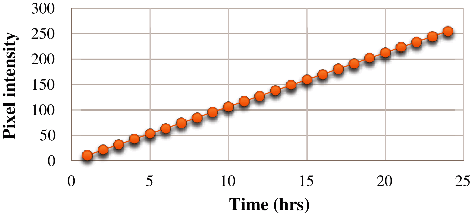
Figure 4: Mutual linear normalization of time and pixel intensity

3.4 Feature Optimization

The process of feature optimization is done by two stages—feature extraction and feature selection, as discussed in the following.

3.4.1 Extracting Features

Feature extraction is the process of getting useful features from existing data. New features are generated by combining and transforming the existing features in the dataset. The raw time-series dataset often is not suitable for direct analysis and comparison. The feature extraction transforms these data into features suitable for modeling. In this work, we used a CNN-based feature extraction scheme.

CNN is comprised of two major portions, a feature extractor and a classification portion. However, we were specifically interested in the feature extractor portion of the CNN model. When using traditional CNN, we do not need to extract and select features; rather, it is done automatically during the training. The features extracted convolutionally are dynamic and are of better quality compared to a model with constant features. Further, this technique can be a good option when we do not have any prior knowledge of the features. This, in turn, can sometimes extract new features that may prove to be beneficial to the model. Since our model only focuses on the feature extraction portion, unlike a traditional CNN model, we needed to introduce a special feature selection model to eliminate the undesirable features that may hinder the model performance.

The input to the considered CNN model is shown in Fig. 5. We considered the stride or the window size as 1, i.e., the data frame window slides for each day, as shown in Fig. 6. Frames represent the number of values considered in a single instance of the model. The architecture for convolutional feature extraction is shown in Fig. 7.

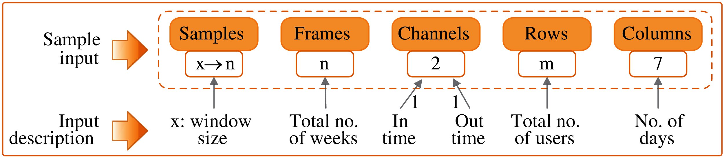
Figure 5: Input parameters for the considered CNN model

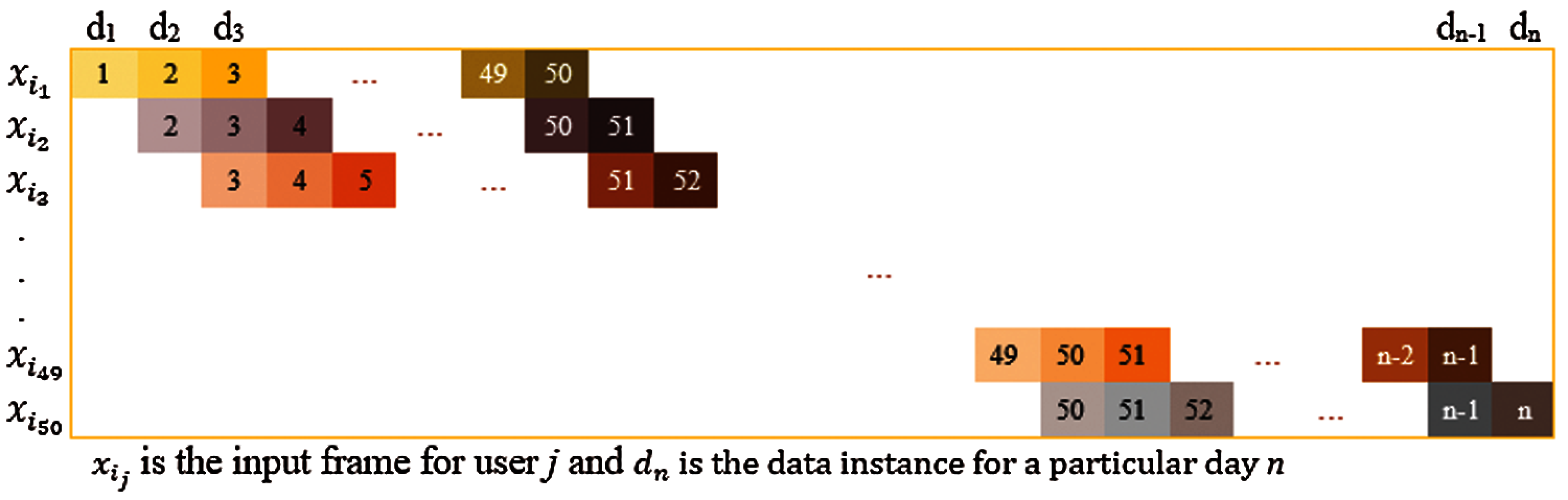
Figure 6: Distribution of the frames for training the feature extractor model

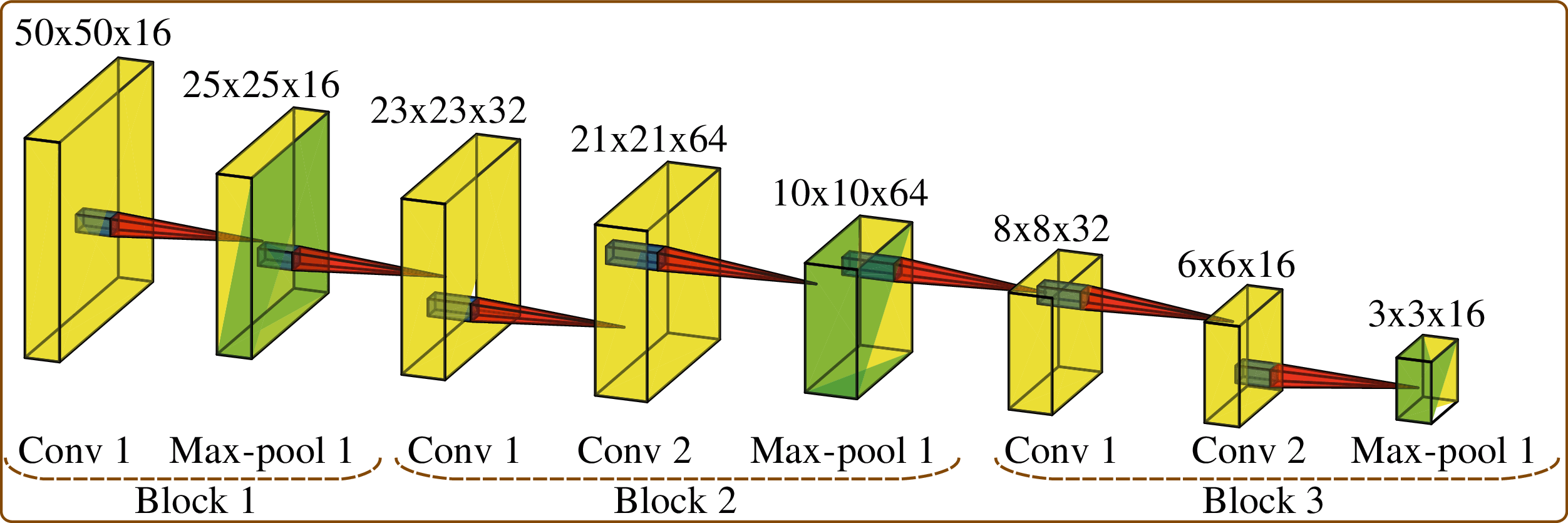
Figure 7: Convolutional feature extraction architecture

For the training, we needed some way to feed the data into the model. Since the total quantity of our input data was restricted to a few months, our training data was serially fed to the model, adding one day at the end and removing one day from the front in each iteration. Considering the input day as dn and the input frame as xim, where i is the number of users, n is the day count, and m is the index of input iteration, the distribution of the frames for training the feature extractor model is represented in Fig. 5.

After the input frames are ready, we moved on to the feature extraction phase. A new technique for the feature extraction model is developed specifically for this work, as represented in Fig. 8. This model contains five main segments, as discussed below:

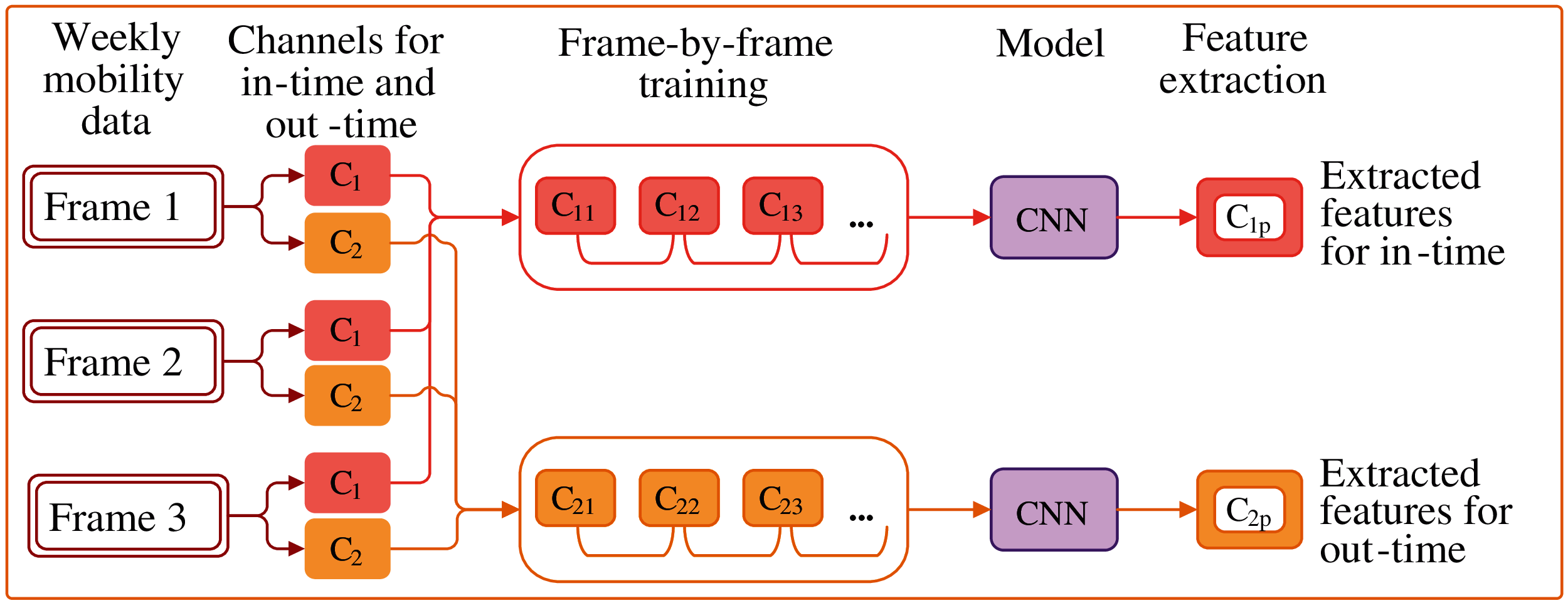
Figure 8: Feature extraction for in- and out-time using CNN

Weekly mobility data: This is the input data frame containing two channels of information, one for in-time and the other for out-time, for all the users in the considered duration.

Channels for in-time and out-time: In this phase, we split the frame into two channels for further extraction. The subsequent functions were repeated for each channel separately.

Frame-by-frame training: To train the model, we distributed the frames to improve the model performance, as shown in Fig. 6.

Model: This is the CNN model for convolutional feature extractor without the classifier, as shown in Fig. 5. The model architecture consists of three blocks of several convolutional and a max-pooling layer, as shown in Fig. 7.

Feature extraction: Each frame component was fed into the model, and the features were extracted. The extracted features were stored in a vector form, which was fed into the GRU prediction model.

3.4.2 Selecting Features

During convolutional feature extraction, the model may contain some features that are either not useful to the prediction model or may cause performance degradation due to multi-collinearity. Feature selection is the process of selecting the most suitable features and removing the unnecessary or redundant features from the feature set. The presence of redundant or irrelevant features decreases the model’s accuracy. Performing feature selection reduces training time, better interpretation of the model, improved generalization, and reduced overfitting.

Though the Ridge and LASSO (least absolute shrinkage and selection operator) regressions are the two natural choices for feature selection, in this paper, we opted for LASSO regression because, in Ridge, the coefficients do not shrink exactly to zero. In comparison, LASSO selects only one among the highly correlated features and shrinks the others exactly to zero. The leftover non-zero values are selected to be used as features in the model. LASSO reduces the variance without increasing the bias much.

The objective function of LASSO is defined by Eq. (1). Here, λ is the tuning parameter that controls the shrinkage. The larger the value of λ, the more the number of features is reduced. After applying the convolutional feature extraction, there was a total of 46,384 features in our considered time-series dataset. Using LASSO, the total number of features was reduced to 4,976.

βLASSO=∑i=1N(yi−∑j=0mxijβj)2+λ∑j=0m|βj| (1)

where, βj={g(β−j)+λ2,if g(β−j)<−λ20,if −λ2≤g(β−j)≤−λ2g(β−j)−λ2,if g(β−j)>λ2

3.5 Prediction Model

3.5.1 CGRU Modelling

CGRU is a formulated time-series data prediction model that uses the convolutional feature extractor of a typical CNN to generate dynamic features. Afterward, these features undergo a special feature selection phase, and finally, the features are fed to the GRU for prediction. This section of the paper describes the GRU prediction model.

Basic GRU Architecture

A GRU unit has two gates—(a) update gate and (b) forget gate. These two gates are trained to retain information from the past without losing it through time and eradicate the irrelevant information that are not needed for prediction. Fig. 9 shows a typical GRU architecture, while its components are briefed below.

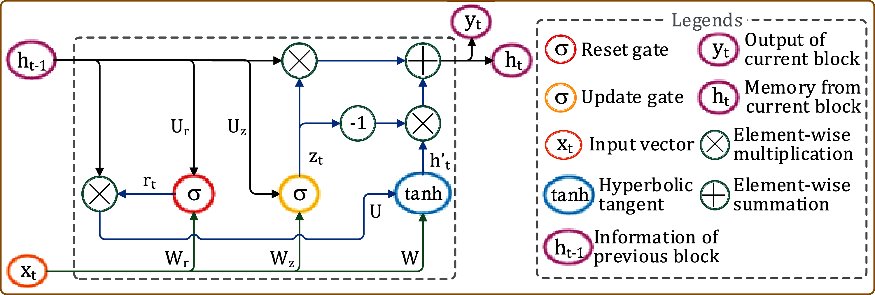
Figure 9: A typical GRU block

•   Update gate: The update gate helps a GRU model determine how much of the past information from the previous blocks need to be forwarded to the next block. This allows the model to decide to copy all the past information and eliminate the vanishing gradient problem. The update gate zt for timestep t is calculated using Eq. (2). Here, xt is the input at step t, and ht−1 is the hidden state that holds the information for the previous t − 1 units. Wz and Uz are the respective weights of xt and ht−1. The sigmoid activation function (σ) helps to keep the value of zt between 0 and 1.

zt=σ(Wzxt+Uzht−1) (2)

•   Reset gate: The reset gate rt is used to decide how much of the past information to forget. rt is calculated using Eq. (3).

rt=σ(Wrxt+Urht−1) (3)

•   Current memory content: The current memory content h′t uses the reset gate to store the relevant information from the past and is calculated using Eq. (4), where ⨀ denotes Hadamard (elementwise) product.

ht′=tanh⁡(Wxt+rt⨀Uht−1) (4)

•   Final memory: The final memory ht at current timestep t is a vector that holds information for the current block and is passed to the next. ht is calculated using Eq. (5). The update gate determines how much information to be retained from current (h't) and previous (ht−1) memory contents.

ht=zt⨀ht−1+(1−zt)⨀ht′ (5)

Proposed CGRU Model

To model the CGRU, we used two layers of the GRU network. Using the CGRU modeling, we aimed to maximize the conditional probability (p(C∣N)) of the convolutional features at the current timestep (C) over the input (N) at the next timestep, as shown in Eq. (6). Here, based on N, the model optimizes the current prediction. To check for improvements, the timestep and the frames of input are modified during the training phase. But for this experiment, the number of input vectors is less; hence, we forwarded with a single stride over the input vectors for each timestep.

p(C∣N)=∏j=1m=p(x(i+j)j,N) (6)

The input to the initial GRU cell is the convolutional feature vector of the input data at timestep t. The input to the next GRU cell is the output of the initial GRU cell, which then passes into a SoftMax layer for classification, as shown in Eq. (7).

p(qt∣(qt+1))=softmax(Wfht) (7)

where, Wf is a learnable parameter, qt is the current GRU cell output at timestep t, ht is the hidden states, and qt and qt+1 are two adjacent input vectors to the model.

The output hidden state at the current timestep is generated using Eq. (8).

ht=CGRU(qt−1,ht−1) (8)

3.5.2 Training

Training a model is to make the model learn the trainable parameters and tuning the hyperparameters. The training phase decreases the error in the training dataset d of size m. The training objective function Tt is represented by Eq. (9).

Tt=∑i=1m−log⁡p(pi∣ai) (9)

where, pi is the predicted output and ai is the actual output.

4  Test Result and Analysis

As discussed in Section 3.1, we used two datasets for understanding the model performance for a lower volume of data. This is important in this problem due to its implementational and usage nature. To measure the model performance, we used accuracy and perplexity as measurement metrics. Accuracy reflects the total number of correct predictions made. Perplexity is used to compare the outputs of the probabilistic prediction models. Here, we used perplexity to represent the prediction loss for an input sample in the current timestep. To improve a prediction model performance, it is desirable to have higher accuracy and lower perplexity.

To evaluate our proposed model’s performance, we considered using these metrics over 20 epochs as the training model perplexity and accuracy did not improve after that. We used training and testing statistics for evaluation, which shows the perplexity vs. accuracy graph for each of the datasets. For comparison, we considered using GRU with 12 epochs without convolutional features and measured its efficacy over CGRU. The training and testing accuracy and perplexity for the GRU and CGRU models are presented in Figs. 10 and 11, respectively. For traditional GRU, the model training accuracy and the testing accuracy are 39.9% and 38.1%, respectively, for 150 days and 33.4%, and 28.9% for 120 days. On the other hand, for CGRU, the model training accuracy and the testing accuracy are 79.7% and 76.8%, respectively, for 150 days and 69.8% and 66% for 120 days.

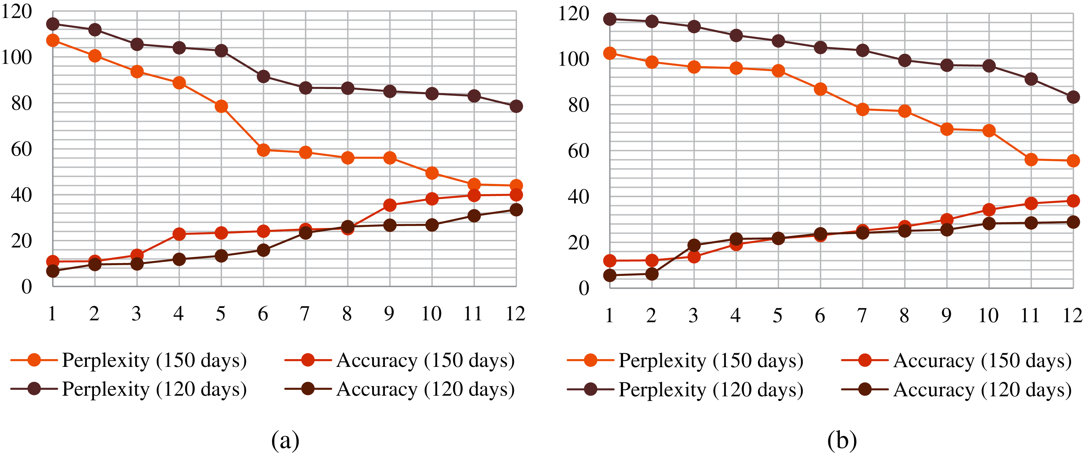
Figure 10: Statistics of GRU for two datasets of (a) Training and (b) Testing

Fig. 12 shows the improvement of the testing accuracy with respect to (a) the number of days of data used and (b) the prediction model used. With an increment of 30 days of data, the GRU model shows a significant improvement of 15.47% over CGRU. This is because the performance of GRU with less amount of test data is very bad. A slight increase in the data volume makes the performance significantly better. Whereas, since the performance of CGRU is already far better than GRU, the increase in data amount does not make much difference in the performance of the CGRU model. For the same reason, when comparing the GRU and CGRU models for 120 and 150 days of data, GRU lacks significantly.

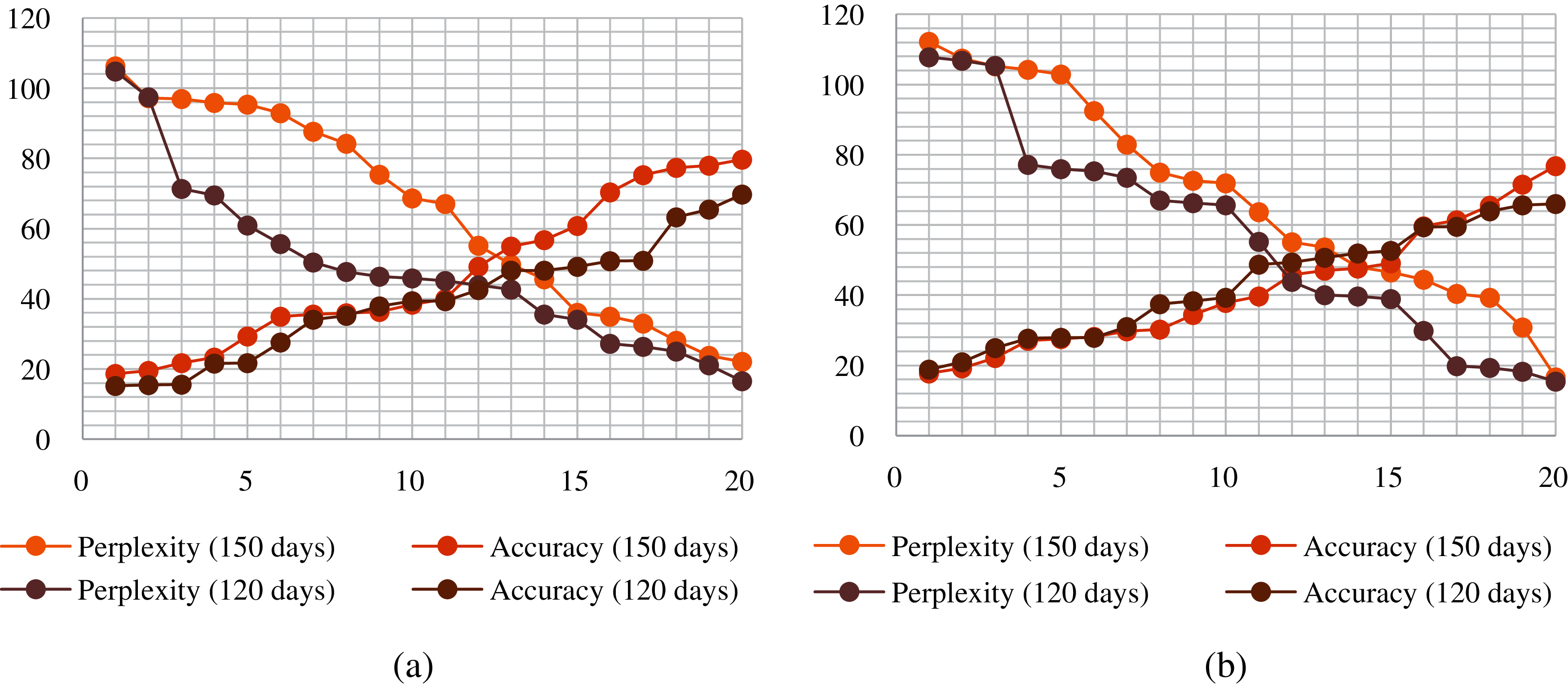
Figure 11: Statistics of CGRU for two datasets of (a) Training and (b) Testing

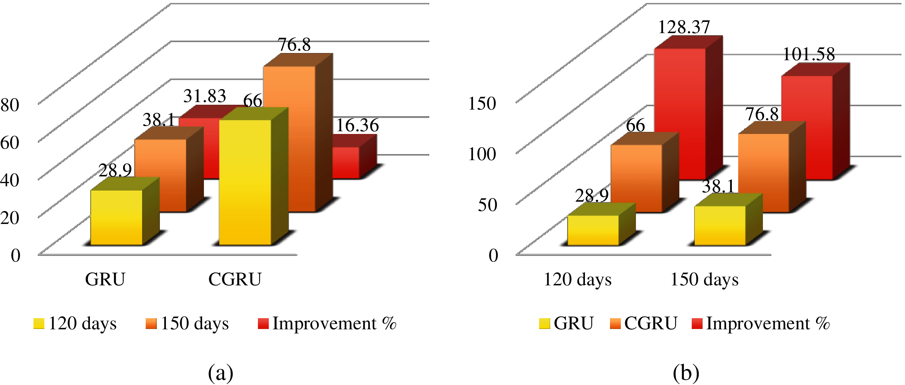
Figure 12: Improvement percentage of testing accuracy with respect to (a) number of days of data used and (b) prediction model used

These statistics prove that CGRU outperforms GRU in both cases when the volume of data is low and high. So, the CGRU-based prediction model is suitable for crowd computing applications where sufficient crowd data is not available.

5  Conclusions

In this paper, we designed a model for predicting mobile devices’ availability in a local mobile crowd computing environment, where the users generally join the network regularly. We presented a novel dynamic feature extraction method where the features are unknown. Based on the extracted and selected features, we considered a convolutional GRU as the prediction model. Our experiment showed that introducing the proposed convolutional feature extractor to the GRU prediction model exhibits significant improvement in the prediction accuracy. For our considered application, the traditional GRU-based prediction model exhibits substantially lower performance accuracy. In comparison, the proposed CGRU model gives satisfactory performance accuracy not only when the dataset is large enough but also for the small-sized dataset. Thus, we can conclude that the proposed CGRU model can be a feasible resource availability prediction model in mobile crowd computing both with small- and large-scale user mobility data.

Funding Statement: This research was supported by Taif University Researchers Supporting Project Number (TURSP-2020/10), Taif University, Taif, Saudi Arabia.

Conflicts of Interest: The authors declare that they have no conflicts of interest to report regarding the present study.

1https://blog.keras.io/index.html

This work is licensed under a Creative Commons Attribution 4.0 International License, which permits unrestricted use, distribution, and reproduction in any medium, provided the original work is properly cited.