Computers, Materials & Continua DOI:10.32604/cmc.2022.019407
Article

Simulation of Non-Isothermal Turbulent Flows Through Circular Rings of Steel

Abid. A. Memon1, M. Asif Memon1, Kaleemullah Bhatti1, Kamsing Nonlaopon2,* and Ilyas Khan3

1Department of Mathematics and Social Sciences, Sukkur IBA University, Sukkur, 65200, Sindh, Pakistan
2Department of Mathematics, Faculty of Science, Khon Kaen University, Khon Kaen, 40002, Thailand
3Department of Mathematics, College of Science Al-Zulfi, Majmaah University, Al-Majmaah, 11952, Saudi Arabia
*Corresponding Author: Kamsing Nonlaopon. Email: nkamsi@kku.ac.th
Received: 12 April 2021; Accepted: 15 June 2021

Abstract: This article is intended to examine the fluid flow patterns and heat transfer in a rectangular channel embedded with three semi-circular cylinders comprised of steel at the boundaries. Such an organization is used to generate the heat exchangers with tube and shell because of the production of more turbulence due to zigzag path which is in favor of rapid heat transformation. Because of little maintenance, the heat exchanger of such type is extensively used. Here, we generate simulation of flow and heat transfer using non-isothermal flow interface in the Comsol multiphysics 5.4 which executes the Reynolds averaged Navier stokes equation (RANS) model of the turbulent flow together with heat equation. Simulation is tested with Prandtl number (Pr = 0.7) with inlet velocity magnitude in the range from 1 to 2 m/sec which generates the Reynolds number in the range of 2.2 × 105 to 4.4 × 105 with turbulence kinetic energy and the dissipation rate in ranges (3.75 × 10−3 to 1.5 × 10−2) and (3.73 × 10−3−3 × 10−2) respectively. Two correlations available in the literature are used in order to check validity. The results are displayed through streamlines, surface plots, contour plots, isothermal lines, and graphs. It is concluded that by retaining such an arrangement a quick distribution of the temperature over the domain can be seen and also the velocity magnitude is increasing from 333.15% to a maximum of 514%. The temperature at the middle shows the consistency in value but declines immediately at the end. This process becomes faster with the decrease in inlet velocity magnitude.

Keywords: Incompressible turbulent flow; heat transfer; non-isothermal; finite element method; energy equation

1  Introduction

The implication of the circular rings or cylinders in the channel of any shape to execute the efficient heat exchanger is extensively used in the field of engineering, science and industry where the improvement of the heat transfer or heat energy is important or beneficial [1–3]. Due to cooling or heating purpose, rectangular heat exchangers have significant roles in the field of spacecraft, power generating industries, refrigeration and cryogenic procedures, food supplier industries, and petroleum industries. To magnify the heat transfer in the rectangular heat exchanger fitted with the circular tubes several fluid dynamics factors are utilized for example pressure drop, flow speed of the particles, different shapes of the geometry, obstacles of regular boundaries and curved shape, different types of flow (laminar or turbulent), different materials of fluid, etc. It is also reasonable to say that convective process, which depends on the heat transfer coefficient possesses, has a direct relationship with the fluid velocity [4–7]. In the cases when flow is examined through turbulence, velocity of the fluid remains increased due to the addition of kinetic energy of the fluid with dissipation rates [8–10]. Due to the turbulence the amount of airflow as well as the blare of the flow are enhanced which stimulates the heat conduction and thermal collaboration. This indicates to control the heat transfer to make the efficient rectangular heat exchanger, the turbulence modeling in the channel plays a vital role [11–13]. Along with the turbulence modeling the making of the heat exchanger with the air as testing fluid with addition of the non-isothermal flow properties carries a lot of importance in numerous applications like making coolant apartments, maintaining the residential heat up, producing ventilated air conditioning rooms, solar collectors, production of the turbine blades running through gaseous, etc. [14–16]. Because of having variety of applications in civil, electrical, and mechanical engineering, different scientists and researchers have put their energy to study (numerically and experimentally) the heat transfer enhancement of the physical problems.

The turbulent flow simulation along with the heat transfer over the circular cylinder was studied by [17] with the large eddy simulation using immersed boundary procedure. To get the experimental data for the turbulence near the cylinder, particle image velocimetry and hot-wire anemometer was used. A large data for the turbulent flow was gathered near the premises of the cylinder. Another experimental study [18] was performed using the laminar region for the heat transfer enhancement of circular cylinder. They intended to find a certain reference temperature that yields the kinematic viscosity that can be used to predict the forces due to convection through the bluff objects. Leading the previous experimental study [19] used the numerical as well as experimental approach by using the different input temperatures with different Reynolds numbers. The study suggested the equation that shows the relationship between the temperature coefficient on the surface of the cylinder and input temperature. On observing the phenomena of vortices [20] due to the alteration of the momentum equations as well as the heat transfer, hot anemometry was used to measure the heat fluxes in the recirculating region and average momentum. With the amplification of the same study [21] observed in detail the alteration of the velocity correlations, Prandtl number for the turbulent and fluctuation of the temperature in the region. It was also added that, due to the momentum created in the region, transport of the heat was greatly affected. From the ancient, many experiments and numerical approaches [22–26] were applied to insert the circular tubes as the tabulator creator or vortex generator to enhance the heat transfer in the rectangular channel in such a way a valuable heat exchanger can be made. Also, much literature [27–29] can be found that developed the correlations among the fluid dynamics parameter and the non-dimensional parameter which might help design the heat exchanger of any shape. Many of the researchers who had focused on the shape of the heat exchanger for example [30–32] have suggested that increasing the heat transfer in the tube dimpled channel proved to be the most beneficial in terms of transferring the heat than the plain tubes. From many of the articles [33–35], it was also discussed that to fit elliptical shells in the tube made the heat exchanger more efficient about 20% than fitting the circular shells in the tube! The heat exchanger is widely used to make diesel engines in mechanical engineering because of its heat energy transformation efficiency. Engineers are laboring hard to make efficient heat exchangers that resist a lot the emissions and raise the fuel capacity of the engines. There are several articles found [36–40] that use the turbulent models with different materials to work out on the heat controlling in heat exchangers.

2  Methodology

2.1 Implementing Physics in the Model Construction for the Channel

The simulation has been expanded to explore the rectangular heat exchanger enclosed by the three circular cylinders of steels for temperature configuration and analysis of fluid flow over these cylinders. The inner radius of all cylinders and thickness is 0.25 [m] and 0.05 [m] respectively. The cylinder at the lower boundary is at the middle of the channel whereas the other two cylinders are placed at 25% and 75% of the total length of the channel at the upper boundary. Air as experimenting fluid is practiced and Flow is considered to be non-isothermal flow where the thermal properties are essentially time and temperature-dependent. For this goal, a rectangular tube is conjectured to have a length of 4 [m] and a height of 1 [m] see Fig. 1. A trial inlet velocity with magnitude in the range from 1 to 2 m/sec with the interval of 0.1 is conceded to enter with the initial temperature Tin = 232 [K] whereas the three solid circular cylinders are initially kept at constant temperature of Tp = 278 [K]. The simulation for such type of fluid flow is based on the questioning to check just for the pattern of velocity field and the temperature distribution on the circular tubes and other variables of interest. The channel is open on the right whereas the pressure is kept zero with stifling the backflow condition. This implies that the fluid and heat can enter and leave from the exit of the channel. Moreover, the symmetrical walls are well insulated.

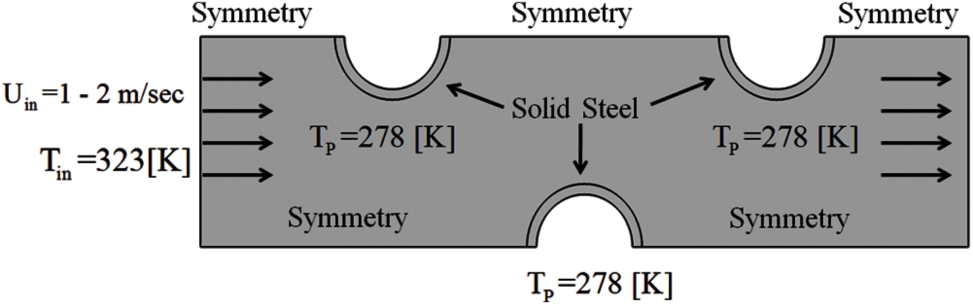
Figure 1: Schematic diagram of the channel with boundary conditions of the turbulent flow and heat transfer

2.2 The Meshing Process and Convergence Analysis

The selected rectangular channel has been meshed with irregular, triangular and the quad meshes. In Fig. 2a the coarse mesh is viewed which is composed of 3126 elements with edge elements of 288. To get the better convergence Fig. 2b, fine mesh is used which is consisting of 12429 elements that are connected through 641 edges and 22 vertex elements. Here, the geometry is composed of 11433 triangles and 996 quads. Here 6950 mesh vertices are used with minimum element quality of 0.1479 and average element quality of 0.8938. Near the circular cylinders we have used more fine mesh in order to have higher accuracy. For simulation using Comsol Multiphysics 5.4, 41913 degrees of freedom are solved with the internal degrees of freedom 841. Tab. 1 represents the convergence plot for the last iteration for some parameter Uin. We achieved excellent results when compared with the available literature.

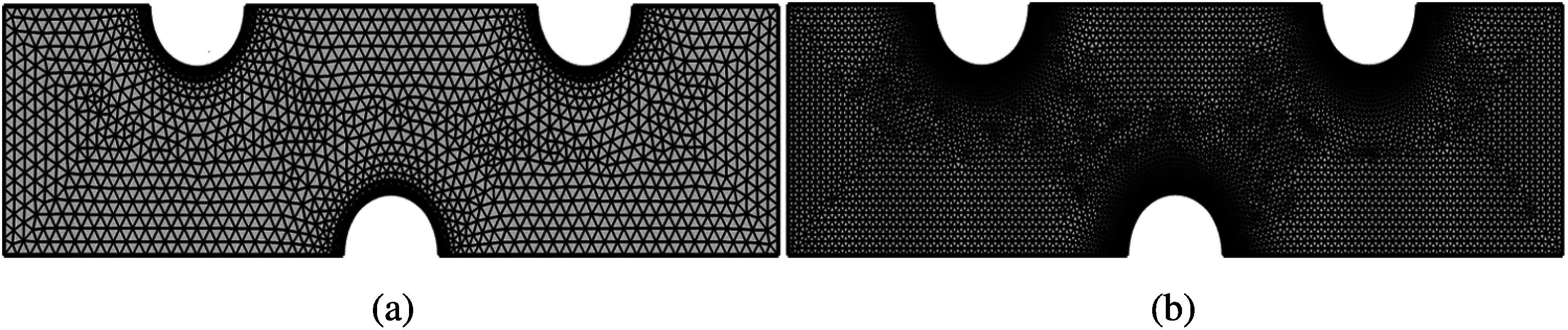
Figure 2: Meshing with irregular triangular as well as quad elements (a) A coarse mesh (b) fine mesh

2.3 Reynolds Navier Stokes Equation and the Standard κ−ε Model of Turbulence Along with Heat Equation in Scalar Form

Turbulent flows are difficult to analyze due to addition of energy terms along with Navier Stokes equations. We might state that the turbulence is another form of energy. Due to the basis of complexity and addition of the energies in the fluid, the simulation through the Navier Stokes equation is controlled by time average quantities. The Reynolds averaged Navier Stokes equation is essential to predict the fluid flow for the turbulence, the idea was given by Osborne Reynolds. The equations are based on the experience for the turbulence flow which divines the approximate solution of the Navier Stokes equation. The equations are acquired with the use of the basic Navier Stokes equations when to write in the Einstein notation in the scalar form:

Continuity equation:∂ui∂xi=0,(1)

Momentum equation:∂ui∂t+uj∂ui∂xj=−1ρ∂p∂xj+∂∂xj(μρ∂ui∂xj).(2)

The derivation of the RANS model is accompanied by the Reynolds decomposition. According to his idea, each variable used to predict the flow can be disintegrated into time-averaged component q−s and fluctuating terms q′. The further hypothesis will be made that the average of the fluctuating terms will be zero i.e., q′−=0. Let all useful quantities in the equations are described into time-averaged and fluctuating terms as:

Reynolds decomposition:ui(xk,t)=Ui(xk)+u′(xx,t),(3)

Ui(xk)=limT→∞⁡1T∫0Tu(xk,t)dt.(4)

Now substituting (3) into (1) and (2) and averaging the quantities we get the following reduced equations.

Continuity equation:∂Ui∂xj=0,(5)

RANS Model:∂Ui∂t+Uj∂Ui∂xj=−1ρ∂P∂xj+∂∂xj(μρ∂Ui∂xj)+∂∂xj(−ui′uj′_______).(6)

Due to the assumption, the fluctuating terms in the RANS model would be omitted. The term in Rij=−ui′uj′_____ Eq. (6) is known as the Reynolds stress, widely used and known as the game-changer of the turbulent flows. To perceive the precise results for the turbulence model, Reynolds stress terms are exercised as the closure of expression (6). With the implementation of the Boussinesq approximation, the Reynolds stress will be associated with gradients of the base velocity of the flow. Let μt be the eddy viscosity then Reynolds stress components can be written as:

Rij=−ui′uj′_____=μtρ(∂Ui∂xj+∂Uj∂xi).(7)

Using (7) in (6) and manipulating the terms we get:

∂Ui∂t+Uj∂Ui∂xj=−1ρ∂P∂xj+∂∂xj(μ+μtρ∂Ui∂xj)(8)

where μt=ρCμκ2ε is eddy viscosiy term. The addition of the eddy viscosity μt will maintain the results in the terms of more precision due to the observation of the turbulence flow. Furthermore, computing the eddy viscosity is relaxed with the numerical as well as an experimental strategy. For the particular problem of the turbulence flow, the standard κ−ε model is practiced. To predict the patterns of interested variables the κ−ε model of the turbulence flow is extensively used because of the more accurate when comparing the practical results and it is very economical due to less computation of the time. Here we present the standard κ−ε model by the Eqs. (9) and (10).

κ-model:∂κ∂t+Uj∂κ∂xj=2μtρ(∂Ui∂xj+∂Uj∂xi)2−ε∂∂xj[1ρ(μ+μtσκ)∂κ∂xj],(9)

ε-model:∂ε∂t+Uj∂ε∂xj=εk[C1ε2μtρ(∂Ui∂xj+∂Uj∂xi)2−C2ε]−∂∂xj[1ρ(μ+μtσε)∂ε∂xj].(10)

In these Eq. (5) variables are chosen to be free or to optimize the results to give better accuracy. For a particular problem we pick them as:

Finally, due to the steady-state computation for the fluid flow and the heat transfer, the time derivative for all the independent quantities would be taken as zero. i.e.,

∂Ui∂t=∂κ∂t=∂ε∂t=0.(11)

To examine the heat transfer problem, the governing steady-state heat equation is accompanied by the κ−ε model and RANS model. We present the heat equation with implication of the Fourier law on it. Let θ denote temperature distribution over the domain with help of velocity field u then heat equation to predict the transfer of the heat in the domain can be written as:

Vector form:ρCpu.∇T+∇.(−k∇T)=0,(12)

Scalar form for isotropic problems:ρCpui∂T∂xi+−k∂T∂xi=0.(13)

Here, k is the thermal conductivity.

Parameter Computation Formula

The heat transfer coefficient will be computed by the following correlation (a famous Dittus-Boelter equation) for the turbulent flows:

hdk=0.023(jdμ)0.8Pr0.4.(14)

where,

d = Hydraulic Diameter of the channel

k = Thermal conductivity

j = Mass flux of the flow per unit area

The local Nusselt numbers and the local Reynolds numbers will be computed by the formula:

Nux=hxk.(15)

Rex=ρuinxμ(16)

3  Validation of the Existing Work with Correlations

To approve the numerical results obtained with the least Square scheme of the finite element method, the two correlations Bejan et al. [41] and Lienhard [42] are used to associate with the present results. According to the provided literature, the local Nusselt number is related to local Reynolds number and with non-dimensional Prandtl number. For the current simulation of the rectangular heat exchanger fitted with three cylinders, the outcomes are estimated and compared with the correlations given by Figs. 3a and 3b at the downstream of the cylinder connected at the lower boundary. The association has been confirmed for the inlet velocities of 1, 1.5 and 2 m/sec see Figs. 3a–3c. It can be inferred that the results gained are in better accuracy with experimental results or with the correlations. It has been asserted that using the Least Square technique of Galerkin's strategy consumes less time for the computation and gives more reliable results. We assume that by practicing FEM via COMSOL Multiphysics 5.4 the results are reliable to some length. On behalf of the comparison with the correlations, we are going to provide some more relationships for the fluid dynamics parameters and the parameters of the thermodynamics.

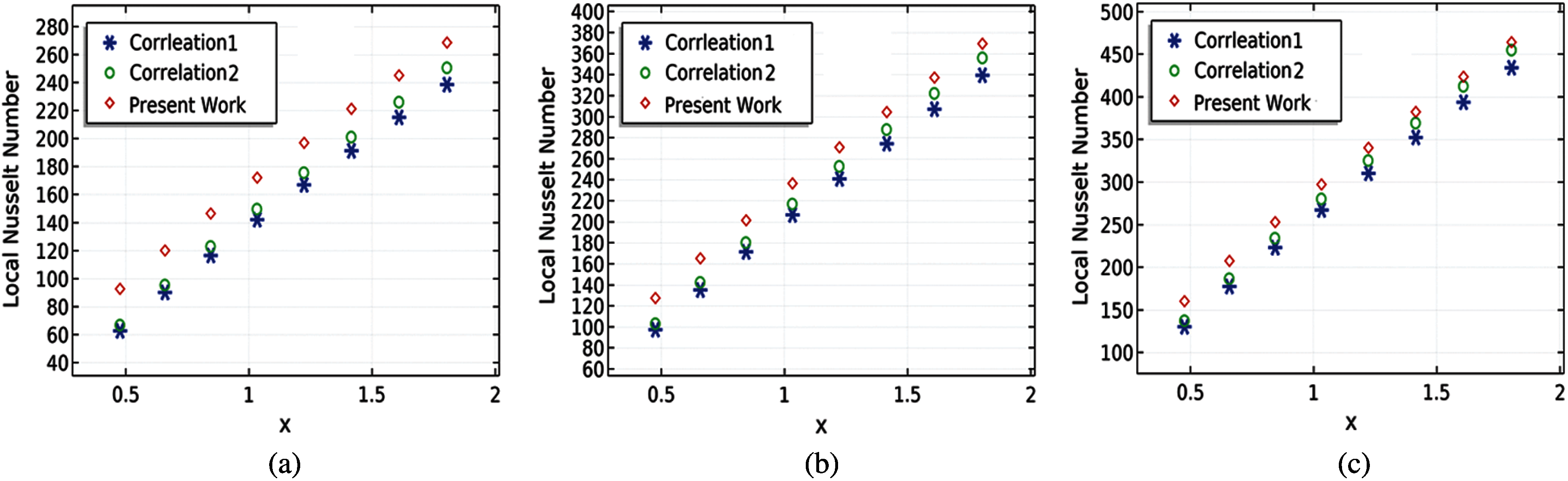
Figure 3: Verification with the experimental correlation with the present work of the Nusselt number (a) uin = 1 m/sec (b) uin = 1.5 m/sec and (c) uin = 2 m/sec

4  Results and Discussion

The current fluid flow problem along with heat distribution is checked by using the turbulent κ−ε model of Reynolds averaged Navier Stokes equations in combination with heat equation for the rectangular domain outfitted with the three semi-circular cylinders comprised of steel at the boundaries of the channel. Two cylinders are attached on the upper boundary centered at 25% and 75% of the lengths while the third cylinder is fitted with lower boundary at the middle of the channel. The inlet velocity magnitude of the channel is assumed in the range from 1–2 m/sec with intervals of 0.1. Consequently, for the current problem, we have formed 11 different simulations for the test. The advantage of such an inlet velocity will produce the Reynolds number from 2.2 × 105 to 4.4 × 105 with the turbulent kinetic energy from 3.75 × 10−3 to 1.5 × 10−2, dissipation rate from 3.73 × 10−3 to 3 × 10−2 and with the fixed Prandtl number Pr = 0.7. The air as the effective fluid is inquired with the inlet temperature of 323 [K] and steel cylinders are assumed at temperature of 278 [K]. The fine mesh is practiced to get a better convergence. The model equations of RANS and two-dimensional energy equations are discretized with the finite element scheme. The whole simulation is stocked on Comsol Multiphysics 5.4. The results are confirmed with the two experimental correlations linking local Nusselt number, local Reynolds number, and Prandtl number. The results are delivered with the help of surface plots and streamlines with arrow plots. The motion of the fluid will be described at the middle of the channel for components of velocity field, pressure and the heat distribution. Variation of the temperature on the circle attached at 75% of the length on upper boundary is expressed against the flow rate of the particles, pressure, local Nusselt number and local Reynolds number.

4.1 Streamlines Surface Plots of the Velocity Field, Contours of Pressure and Isothermal Lines of Temperature

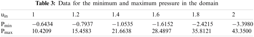
The velocity field streamlines with the arrow and surface plots are exhibited in Figs. 4a–4d. For each input velocity in the domain, the velocity at the outlet is improved by a maximum value of 333.5% see Fig. 4d. The rate of flow is enhanced and move in the recurrent direction of flow. Such an adjustment of the flow will be convenient where the heat energy at the outlet is maximized. The circular cylinders generate restraint in the way of flow and create the hydraulic jumps. Hydraulic jumps after one and another period generate more kinetic energy in the flow. Thus, a dynamic growth in the velocity of the flow in terms of percentage obtained of 333.5% when to elaborate on the basis of inlet velocity. It is the part of the turbulent flows that they are often depending on the velocity given at the inlet of the channel. It is manifest in Fig. 4a. with the given velocity of the 1 m/sec, the velocity at the outlet is extended by 4.26 m/sec. In Fig. 4b. with the given inlet velocity of 1.4 m/sec, the velocity at exit is increasing to 6.14 m/sec. That is the gain of about 514% of the inlet velocity. The minimum and the maximum values in the domain is given by the Tab. 2.

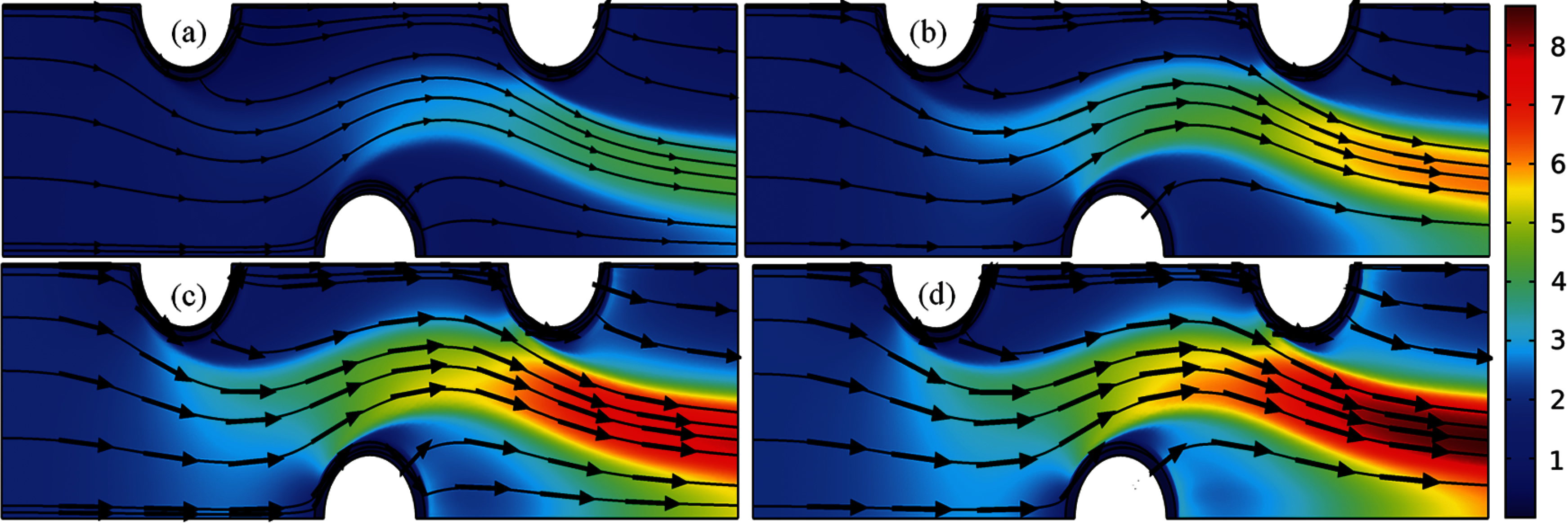
Figure 4: Streamline presentation of the velocity field with the surface plots (a) uin = 1 m/sec (b) 1.4 m/sec (c) 1.8 m/sec and (d) 2 m/sec

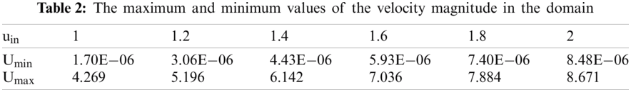
In Figs. 5a–5d the contour plots for the pressure distribution over the domain is presented for the particular velocities at the inlet of 1 m/sec, 1.4 m/sec, 1.8 m/sec and 2 m/sec. For each input velocity in the simulation the flow starts with maximum magnitude in the domain. As the fluid moves to the exit of the channel the pressure is declining down up to a negative pressure. Production of the negative pressure will support the controlling of the fluid inside the pipe. The negative pressure is mostly producing at the end of the channel on the upper corner beside the cylinder. The rapid variation of the pressure can be seen on the space bounded by the three circles due to the rapid increase of the flow rate around the corners of cylinders. Tab. 3 presents the numerical computed results for the minimum and maximum pressure on the whole domain. It is clear that with the increase in inlet velocity the minimum pressure around the domain is decreased whereas the maximum pressure is increased with the increase in inlet velocity magnitude. The portion where the minimum pressure exits may located at the end of the corners of the channel whereas the maximum pressure can be located portion near the inlet of the channel before the first circular cylinder.

Figure 5: Contour plots for the pressure distribution over the rectangular heat exchanger at (a) uin = 1 m/sec (b) 1.4 m/sec (c) 1.8 m/sec and (d) 2 m/sec

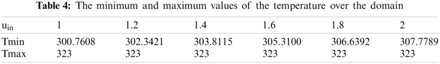
The isothermal contours are exhibited in Figs. 6a–6d for some selected inlet velocities. They are determining that the distribution of the temperature is not uniform across all the domains. But with the rise in inlet velocity, the extent of the temperature intensity is increasing over the domain. Originally, the cylinders are kept at the temperature of 278 [k] whereas the air infiltrates the region bearing the temperature of 323 [k]. As soon as the fluid is passed to enter the region the distribution of heat flows quickly over the domain. The method of distribution becomes quick with increasing the velocity magnitude at the exit of the channel. The minimum and maximum temperatures at the domain of the channel are given in Tab. 4. With the rise of the input velocity, the minimum temperature is growing but there will be no impact on the maximum temperature. The minimum temperature can be perceived at the region surrounded by the circle or at the region after the circle attached at the end see Figs. 6a–6d.

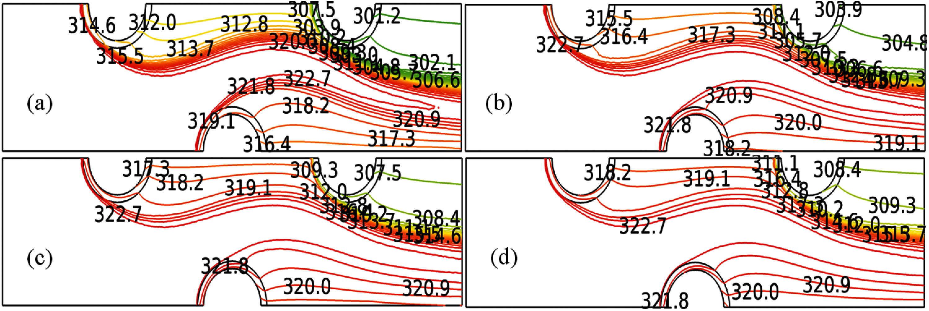
Figure 6: Isothermal presentation for the temperature distribution over the domain at (a) uin = 1 m/sec (b) 1.4 m/sec (c) 1.8 m/sec and (d) 2 m/sec

4.2 Variation of the Temperutre on the Surface of the Cylinder

In the portion we are working to explain the changing of temperature over the surface circular cylinder attached at 75% of the length of the channel against the velocity magnitude, pressure, local Nusselt number and the Reynolds number see Figs. 7a–7d. The temperature of the surface is increasing with the increase in the flow rate of the fluid. The speed of the flow at the center of the cylinder attained maximum and then the temperature declined slowly with the reduction of velocity field magnitude see Fig. 7a. With the increase of pressure on the surface of the circular cylinder, the temperature confers a positive response. With the increase of inlet velocities, the connection between the temperature and pressure bestows more stability and response in the terms of enrichment. The pressure on the surface of the circular cylinder diversifies in a wide range when the velocity magnitude at the inlet is a little boosted.

The convective process is lagging over the surface of the cylinder for each inlet velocity. See Fig. 7c which concludes that the temperature over the cylinder is declining with the increase in local Nusselt number. With enhancing the velocity magnitude at the inlet, the local Nusselt number shows the direct correlation with the temperature. For the current problem of fluid flow and heat transfer, the local Nusselt number varies from 50 to 400 when the inlet velocities are varying in range from 1 to 2. The local Reynolds number behaves the same as the local Nusselt number at the surface of the cylinder. The influence on the temperature of the local Reynolds is identical and with the raising the range of Reynolds number the temperature on the surface decays in the same way as the local Nusselt number does see Figs. 7c and 7d. With the increase in the velocity at the opening of the channel, the range in the local Reynolds is increased with the new derivation of the initial temperature on the surface of the cylinder. It is also apparent that due to the declination of local Reynolds numbers the temperature at the appropriate inlet velocity also operates down with the common pattern for all Reynolds numbers.

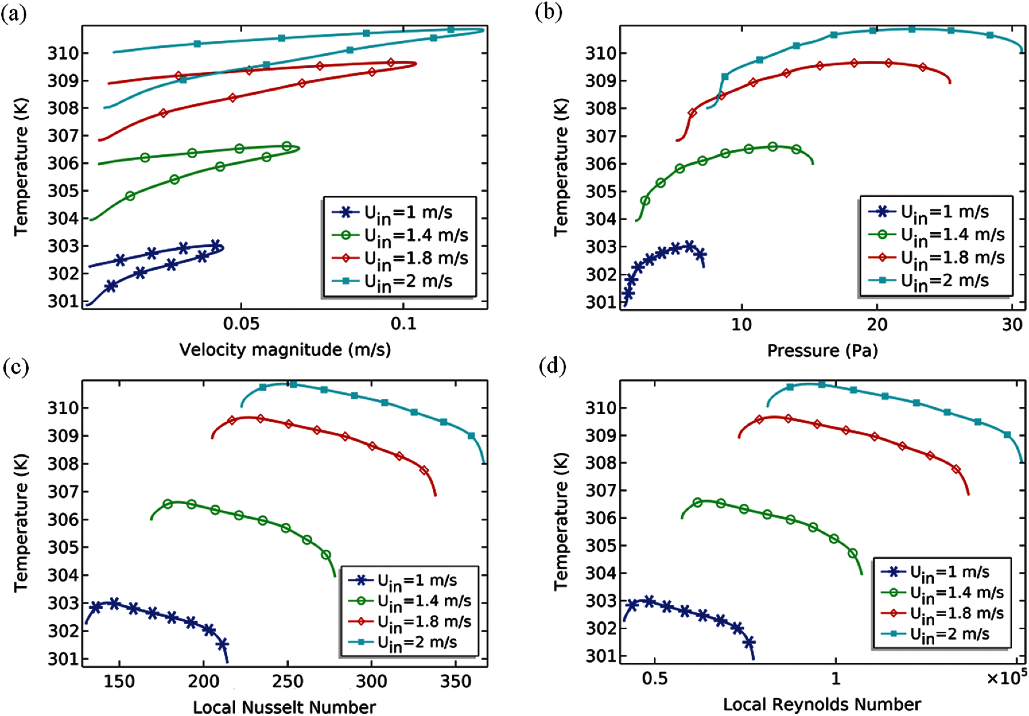
Figure 7: Variation of the temperature on the surface of the circular steel at the selected uin against (a) velocity magnitude (b) pressure (c) Local Nusselt number (d) Local Reynolds number

4.3 Pattern of the Flow in the Middle Horizontal Line of the Channel

It is to assert that while the fluid is departing the region the whole model of the flow can be analyzed in the best fashion in the middle of the channel. Because the motion of the fluid is adjusted in that circumstantial direction. In the part we are going to perceive the pattern of flow for u and v components of velocity pressure and the temperature at the middle of the channel in terms of presented input velocities see Figs. 8a–8d. It is shown in Fig. 8a when the air is deducted to flow the u-component of the velocity is equal to inlet velocity because of the horizontal orientation of the channel. For a particular inlet velocity Uin = 1–2 m/sec, the u-component of velocity is raised while passing the narrow paths enclosed by the three cylinders. It endeavors some optimum values and then declines.

It is also noticeable that the greater the velocity greater the achievement of optimum values of the flow rate over the domain. While inspecting the velocity in y-direction it starts from zero for all given inlet velocities. The y-component of velocity moves in oscillating paths and attempts some minimum values before arriving at the exit of the channel. From Figs. 8a–8b it is inferred that the fluid is mostly stretched towards horizontal paths due to the contraction of the circles. It is apparent from Fig. 8c, the greater input velocity will start the flow with greater pressure but the pressure wanes to zero at the end of the channel. Also, the rate of drop of the pressure is directly proportional to the velocity magnitude at the inlet of the channel. It can be recommended that to start a flow with maximum acceleration a pressure of very less value must be forced at the end of the channel. The temperature distribution acts at the middle with the constant temperature of 323 [k] unless the fluid particles passed by the region molded by the three circles see Fig. 8d. The rapid declination of the temperature can be observed near the exit of the channel refer Fig. 8d. Fig. 8d is also intimating that the less the inlet velocity greater the rapid declination in the temperature down the exit of the channel.

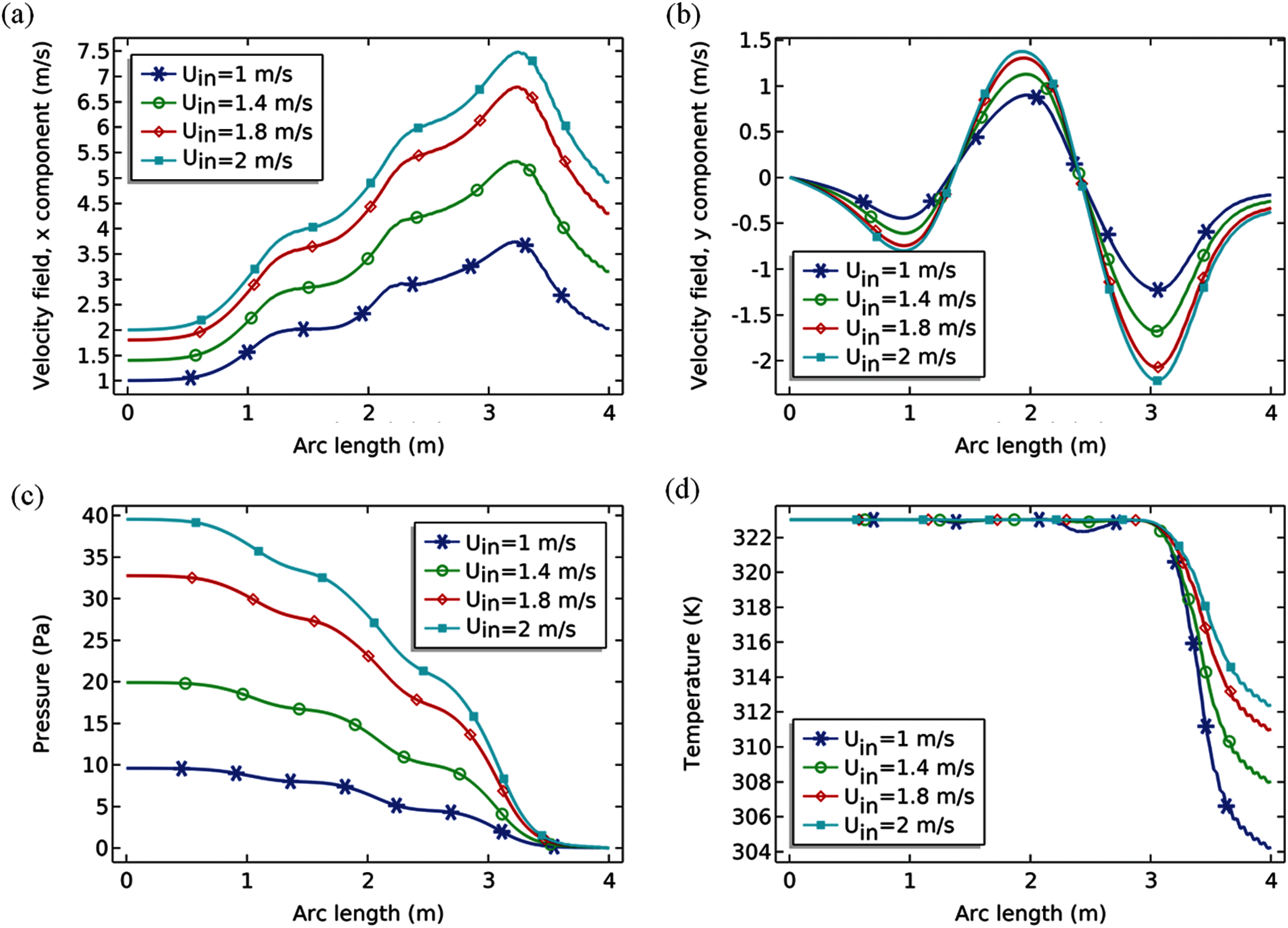
Figure 8: Pattern of the flow at the position y = 0.5 [m] against the selected uin for (a) x-component of velocity (b) y-component of velocity (c) pressure and (d) Temperature

5  Conclusion

The heat flow with the help of air flow was discussed with the use of non-isothermal interface in the finite-element based software Comsol Multiphysics 5.4 which implements the Reynolds averaged Navier Stokes model for the κ−ε turbulence model along with heat equation. A rectangular channel fitted with three circular metallic cylinders, one at the lower boundary at the middle of the channel and two are attached at 25% and 75% of the total length of channel at upper boundary. Such an arrangement can be made to construct the feasible rectangular heat exchangers for cooling and heating purposes. The air as the testing fluid was induced with the inlet velocities in the range from 1–2 m/sec which yields the high range of the Reynolds number from 2.2 × 105 to 4.4 × 105 with the kinetic energy for turbulence in the range from 3.75 × 10−3 to 1.5 × 10−2 and with dissipation rate in the range 3.73 × 10−3 to 3 × 10−2. The cylinders are initially set at the constant temperature 278 [k] and the air is allowed to enter with temperature 323 [K]. The two correlations for the local Nusselt number were compared with the present work and concluded that our numerical results with the good convergence are in good agreement with the experimental results about 20% of the error. The results are presented for streamlines with surface plots of the velocity field, contours for pressure and isothermal lines for temperature distribution over the surface. The course of the temperature was also expressed in terms of velocity magnitude, pressure local Nusselt number and Reynolds number at the upper boundary of the last circle for inlet velocities. At the middle of the channel the velocity components, pressure and temperature were expressed against the length of the channel. We write the following findings from the simulation.

(1)   The discussion of the streamlines pattern and the surface plots indicated that the velocity magnitude is increasing in the range of 333.5% to 514% and due to such arrangement of the cylinders creates the more hydraulic jumps to accelerate the fluid motion. The Rapid variation in the pressure can be seen in the region which is surrounded by the cylinder. For the current problem of the turbulent flow quick distribution of the temperature was seen in the domain.

(2)   When to express the distribution of the temperature over the circular cylinder against velocity it is found that temperature is maximum at the middle of the cylinder. With the increase in the pressure the temperature of the cylinder is increasing for each input velocity. The range of the pressure is also increasing with the increase in input velocity field. Temperature on the surface of the circular cylinder declines due to increase in local Nusselt number as well as the Reynolds number for each input velocity. But for each input velocity the range for local Reynolds number as well as the local Nusselt number is increased.

(3)   Since the channel is horizontal therefore the x-component of the velocity plays a major role in developing the flow at the start of the channel in the middle line and increase in magnitude during the whole flow. Whereas the y-component of the velocity is starting from zero position and remain fluctuate in the domain. The pressure at the middle line is increasing with inlet velocity magnitude and will be zero at the exit of the channel. The temperature in the middle line remains at the same value given at the inlet and declines quickly before reaching at the domain.

Acknowledgement: Authors are very much thankful to Sukkur IBA University, Sukkur, Pakistan for providing conducive environment for research.

Funding Statement: The authors received no specific funding for this study.

Conflicts of Interest: The authors declare that they have no conflicts of interest to report regarding the present study.

This work is licensed under a Creative Commons Attribution 4.0 International License, which permits unrestricted use, distribution, and reproduction in any medium, provided the original work is properly cited.