DOI:10.32604/cmc.2022.020782
| Computers, Materials & Continua DOI:10.32604/cmc.2022.020782 | |
| Article |
Price Prediction of Seasonal Items Using Machine Learning and Statistical Methods
Faculty of Computers and Informatics, Zagazig University, Zagazig, Egypt
*Corresponding Author: Ahmad Salah. Email: ahmad@zu.edu.eg
Received: 07 June 2021; Accepted: 08 July 2021
Abstract: Price prediction of goods is a vital point of research due to how common e-commerce platforms are. There are several efforts conducted to forecast the price of items using classic machine learning algorithms and statistical models. These models can predict prices of various financial instruments, e.g., gold, oil, cryptocurrencies, stocks, and second-hand items. Despite these efforts, the literature has no model for predicting the prices of seasonal goods (e.g., Christmas gifts). In this context, we framed the task of seasonal goods price prediction as a regression problem. First, we utilized a real online trailer dataset of Christmas gifts and then we proposed several machine learning-based models and one statistical-based model to predict the prices of these seasonal products. Second, we utilized a real-life dataset of Christmas gifts for the prediction task. Then, we proposed support vector regressor (SVR), linear regression, random forest, and ridge models as machine learning models for price prediction. Next, we proposed an autoregressive-integrated-moving-average (ARIMA) model for the same purpose as a statistical-based model. Finally, we evaluated the performance of the proposed models; the comparison shows that the best performing model was the random forest model, followed by the ARIMA model.
Keywords: ARIMA; machine learning; price prediction; random forest; ridge; support vector regressor
Today, making a decision about buying or selling any assets or gifts is a very difficult process. A lot of factors and complexities can influence your decision, such as the best time for buying or selling the products, goods, or seasonal gifts. In the financial market, the shareholders need to know when to sell, and the customers need to get the products at good prices. Thus, the price prediction issue has arisen. Price forecasts for trading stocks and commodities were primarily based on intuition. As trading grew, individuals tried to find methods and tools which could accurately forecast the rates, increasing their gains and reducing their risk. Many methods such as fundamental analysis, technical analysis, information mining, statistical approaches, and machine learning techniques are used for price predication. The most hopeful results of forecast systems might be a shift in people’s state of minds [1].
As discussed above, several methods can be used to resolve the price forecast issues, but we will focus on only two: statistical models and machine learning models. There are plenty of machine leaning models for evaluating and forecasting costs. Machine learning models can gain from historic correlation and patterns in the data to make data-driven forecasts or choices [2].
Regression analysis is widely used for forecasting and prediction, where its use has a high degree of overlap with machine learning. Regression analysis is likewise used to find the function that maps the independent variables to the predicted (i.e., dependent) variable, and to find out the forms of these relationships/functions. In limited circumstances, it can be used to identify causal functions/relationships between the independent and dependent variables. In many of applications, particularly with little results or concerns of causality based upon observational data, regression techniques can provide deceptive outcomes. Regression designs for forecast are often helpful even when the assumptions are reasonably breached, although they might not be carried out optimally [3].
Many researchers have explored the problem of price prediction issues with the aid of various machine learning approaches. For example, in [4], the authors forecast the carbon price utilizing the LSTM model on a real dataset of China. In [5], the authors used three machine learning methods: Artificial Neural Network (ANN), SVR, and random forest on cars and truck rate predictions. In [6], many machine learning methods were utilized to forecast the rate of air travel. (e.g., Multilayer Perceptron (MLP), Extreme Learning Device (ELM), random forest, bagging regression trees, and direct regression).
Statistical methods for price prediction problems in [7] were predicting next-day electricity prices based on the ARIMA methodology. In [8], the authors proposed using the ARIMA model and the SVMs model in forecasting stock prices. Several research works utilized the ARIMA model for the task of price prediction.
In the literature, many studies have focused on the subject of price prediction for a variety of financial instruments (e.g., stocks and gold), using a variety of forecasting techniques. Examples include price forecasting for coal, electricity, natural gas, houses, cars, prediction of Bitcoin prices, and second-hand ecommerce price projection.
Despite these efforts, there is no existing research providing a model for predicting the prices of seasonal goods, to our best knowledge. Thus, there is a vital need for models that can predict the prices of seasonal goods and the ability to compare the performance of the machine learning model against the statistical models. These proposed models can help the seller evaluate the proper seasonal goods pricing, which attracts clients and increases profits based on historical data. Historical data of seasonal goods pricing can guide the seller to select the most suitable prices.
In this vein, we framed the task of predicting the price of seasonal goods as a regression task. We proposed a system for predicting the prices of the seasonal items using both machine learning methods and statistical methods. The proposed system utilized a real-life dataset of Christmas gifts. In addition, the proposed work utilized a set of machine learning models and the ARIMA statistical model price. The proposed models are thoroughly evaluated on different evaluation metrics. The main contributions of this paper can be summarized as follows:
1. To the best of the authors’ knowledge, we proposed the first price prediction models of seasonal goods.
2. We provided a comparison between the machine learning-based model and the statistical-based model to learn which model type resolves the problem better.
3. The proposed models are evaluated on several performance evaluation metrics.
The rest of the paper is organized as follows. Section 2 presents a brief theoretical background, explaining the methods and algorithms used. Section 3 describes the related work of price prediction. We exposed the proposed work in Section 4. Section 5 shows and discusses the results. Finally, Section 6 concludes the contributions of this study.
This section provides an overview of the regression methods utilized in this article. The background discusses the theory behind the following algorithms: Linear regression, ridge regression, support vector regression (SVR), random forest regression (RF), and ARIMA algorithms.
The fundamental premise of this regression method is to forecast an interesting time-series
In Fig. 1, the coefficients
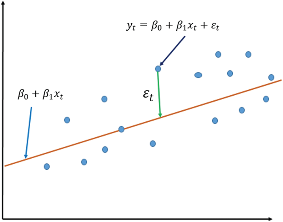
Figure 1: Linear regression model
The observations in Fig. 1 do not form a straight line but are strewn around it. Consider that the observation
The Ridge regression method is a widely used algorithm for resolving the linear regression model’s multicollinearity issue [10]. Hoerl et al. [11] introduced the ridge regression model at the beginning. Essentially, ridge regression is a straightforward amendment of the basic least squares regression algorithm, where the linear model’s parameters are:
Being approximated by the solution of the classic linear least squares equation [12]:
where
The ridge regression model works by framing the following equation an optimization problem, and the target is to minimize the objective function below:
With regard to
K is positive constant. The solution to Eq. (5) yields the estimate for the ridge, which is defined as:
where
where
The regression is a widespread categorization of machine learning models, where the main difference between the regression task and other tasks is that the regression output is continuous. On the other hand, the output of the classification task is discrete, from a finite set. Generally speaking, an ongoing multivariate function is estimated using a regression model. Vector machine support solves difficulties of binary classification by presenting them as issues of convex optimization. The optimization challenge involves determining the largest margin between the hyperplane and properly categorizing as many workouts as possible. SVMs with support vectors represent this ideal hyperplane. SVM generalization to SVR is achieved with the introduction of an e-insensitive area, dubbed the e-tube, as shown in Fig. 2. This tube reformulates the issue of optimization to identify the tube best adapted to the continuous function while balancing the complexity of a model with an error in prediction [14].
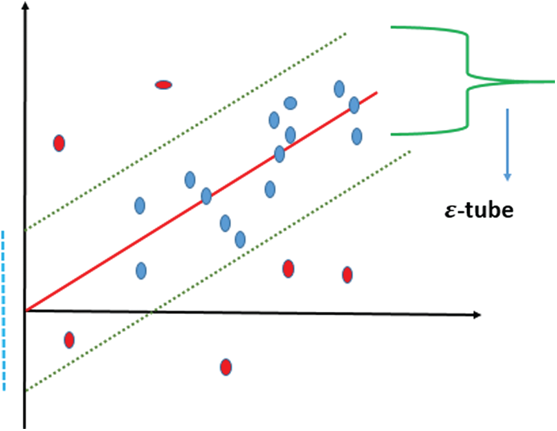
Figure 2: The SVR model
SVR uses an e-insensitive reduction function to address regression problems. This functionality makes it possible for an endurance degree to make mistakes not more than
When employing the ɛ-insensitive loss function, the objective is to design a function that fits the present training data with a deviation smaller than or equal to ɛ, while remaining as flat as feasible. This implies that one desires a small weight vector w. One technique to accomplish this is to minimize the vector’s quadratic norm w. Due to the possibility that this task is infeasible, slack variables
where
The dual variables are denoted by
The random forest (RF) regression method is a kind of ensemble learning in which a large number of regression trees are combined. A regression tree is a collection of criteria or constraints that are grouped hierarchically and applied sequentially from the root to the leaf of the tree. The RF starts with a large number of bootstrap samples selected at random from the original training dataset. Each of the bootstrap samples is fitted using a regression tree. For each node in the tree, a tiny subset of the entire set of input variables is randomly picked for binary partitioning [16].
For forecasting, the ARIMA approach makes use of prior values in the Series. George Box and Gwilym Jenkins devised it, and it is a commonly used forecasting model [17,18]. The ARIMA model is composed of two components: auto-regressive AR terms and moving average MA terms.
Using the lag operator denoted L; Autoregressive AR terms are lagged values of the dependent variable and refer to it as the lag order p, which is the number of time delays. The following formula may be used to express a non-seasonal
Moving Average MA terms are lagged forecast errors in forecasts between actual past values and their predicted values, and they are referred to as the order of moving typical q. A non-seasonal MA(q) can be created as follows:
where
where q, d, and p are positive numbers greater than or equal to zero that denote the order of the model’s autoregressive, integrated, and moving average components. The number d specifies the degree of differentiation [19]. The different series represents the change in the original series’ successive observations. If the initial data are not stationary, we may use first order difference or second order difference processes, and so on. When d equals 0, the model becomes an ARMA (p, q) model. The ARIMA model is an extension of the ARMA model that incorporates non-stationary data [20].
Auto-Correlation Functions (ACFs) and Partial Auto-Correlation Functions (PACFs) are typically utilized to identify the dependence of a time series variable on its history. The fixed time series’ autoregressive and moving average terms are identified by observing the patterns in the graphs of ACFs and PACFs. Autocorrelation is the connection between time series and the lag of the very same time-series, while partial autocorrelations are the correlation coefficients between the standard time series and the lag of the exact same time series, but without the effect of the members in between. The ACF, which is a bar chart of time series of coefficients of connection of time-series and lags of itself, and the PACF, which is a plot of partial coefficients of correlation of time-series and lags of itself, can be used to identify the variety of AR and MA terms [19].
In this section, we discuss the related work of price prediction using machine learning and deep learning method. First, we expose several works utilizing the classic machine learning methods such as SVR, ANN, and decision trees. Second, we discuss the methods utilizing the deep learning techniques for predicting product prices.
Regression analysis is commonly utilized for predictive and forecasting purposes. Regression analysis may be implemented in many different ways. When applied to smaller effects or observational data, regression techniques may produce deceptive results, especially in multiple applications. There is no universally agreed upon real form of the data-generating process, and assumptions may be tested if sufficient data are supplied. Even when the assumptions of a model are only somewhat violated, the regression models may still be beneficial in pricing prediction. Because incorrect conclusions are possible, use caution when using these models. For instance, in some circumstances, correlation might be of use even though it is not directly related to correlation. Regression analysis techniques will provide better results if you have random or semi-random data producing random or semi-random data.
The authors of [21] aimed to develop effective models for predicting housing prices. The facts found in this report provide interesting insight into the Melbourne property market. Appropriate models of regression are used to identify those that are effective. The data set consisted of stepwise linear regression, stepwise polynomial regression, stepwise regression tree, and SVR, which were given a selection of attributes from the dataset. Reduction strategies were utilized to improve interpretability and increase prediction model performance. Boosting and stepwise were also utilized. Once the dataset is cleaned, it is split into two sets: the training set and the test set. Cross-validation was employed for both data reduction and model development, as well as for validating model predictions. Regression tree and neural network were comparatively quicker when compared to SVM. Stepwise, SVM took longer to train than PCA and SVM.
In [22], the authors used a Naive Bayes classifier for sentiment scores, followed by a neural network application of that classifier to both the sentiment scores and historical stock market information. Additionally, the authors focused on the use of the Hive ecosystem for cleaning data. This neural network was being built on top of this pre-processing environment. Using sentiment analysis and historical data, prices were projected. Studies have shown that, under optimal conditions, the model achieves an accuracy level over 90%. It has also been observed that, if the model is trained using the current data, it may provide a robust basis. While sentiment analysis using neural networks is utilized to create a statistical connection with a stock’s historical numerical data records and other elements that affect stock prices, they are also put to use in constructing the aforementioned relationship.
Data-driven methods for predicting natural gas prices were described in [23]. ANN, SVM, gradient boosting machines, and Gaussian process regression were all used in their machine learning efforts. The model was trained using cross-validation. Four forecasting performance metrics are used in prediction methodologies: R-squared, mean squared error, root mean squared error, and mean absolute error. SVM and ANN anticipate the outcome better than GBM and GPR, which are tied for the poorest performance. With regards to ANN, it is well known that it has an innate aptitude for self-study, self-adaptation, and self-aggregation.
A 24-year time-series dataset was used to build the decision tree (DT) model to anticipate crude oil prices in [24]. Economic variables, such as oil prices, are believed to influence the output of the decision tree. Decision trees, random forest, and random tree, among others, were examined to find the most suitable DT algorithm. The accuracy of the DT’s was proven by these results, which showed that the DT’s could be deployed with a high degree of accuracy in the forecast of the West Texas intermediate price. Five classification decision trees were investigated: M5P, random forest, random tree, REP-Tree, and random tree. The random DT model produced the quickest calculation times.
In [25], the authors offered a review on well-known and useful regression approaches, such as polynomial, a radial basis function, sigmoid, and linear regressions that may be used to anticipate stock price movements. The technical analysis approach uses historic prices of stocks such as close and open prices, volume of trading, and adjusted close prices. The second class of analysis was quantitative, which is conducted on the basis of external aspects such as company profile, market situation, and political and financial elements. Machine learning methods in this area have actually shown to enhance performances by 60%–86%, as compared to past methods. To enhance the anticipated cost worth’s accuracy, brand-new variables were constructed by integrating existing variables. ANN is used to forecast the stock’s following day closing price, and RF is also utilized for contrast analysis. Comparative analysis utilizes the root mean square error, MAPE, and MBE values [26].
In [27], the authors utilized deep learning methods for prediction of second-hand items. Online shopping markets provide countless products for sale each day. It is essential for sellers to correctly approximate the price of second-hand goods. The authors proposed a model employing a deep neural network architecture that includes long short-term memory (LSTM) and convolutional neural network architecture. It exceeds all other models with a considerable efficiency gap. First, the authors framed the price prediction of pre-owned items by thinking about the features for a set of items. Then, they established a framework for anticipating the prices of items for a particular product category. They used a prediction model to forecast the quality of an item.
In [28], a hybrid approach based on machine learning and filtering methods was proposed to predict the stock exchange rate. Defensively, the method combined SVR and the Hodrick–Prescott filter. The design offered excellent precision of stock exchange price prediction with an extremely minimalist execution time. It significantly improves the accuracy of anticipating stock market rates. It was based on machine learning and filtering techniques utilizing a novel hybrid method. The proposed design is an efficient predictive perspective solution for stock market rates.
In [29], the SVR was used to forecast stock rates for big and small capitalizations. Computationally intensive methods, using past rates, have actually been established to assist in strongly preferable management of market threat for investors and speculators. This study used SVR and determined its efficiency on numerous Brazilian, American, and Chinese stocks with different qualities. The predictive variables were determined utilizing TA indications on possession costs. The results reveal the magnitude of the mean squared errors for the three well-known kernels in the literature, utilizing specific model training strategies.
The research study’s independent variable was the closing rate of Bitcoin in USD as figured out by the CoinDesk Bitcoin Price Index. Efficiency evaluations of designs were carried out in order to determine their effectiveness. Data referring to the blockchain, consisting of the mining difficulty and hash rate are provided. The aim of the research work was to define new performance measures that might be beneficial to traders. Deep learning models such as the RNN and LSTM are effective for Bitcoin prediction in USD. LSTM surpassed RNN, but not substantially. Information of this nature is currently being gathered from CoinDesk on a daily basis for future usage. The data are not offered in a useful or real-time setting for predicting the future. The performance benefits acquired from the parallelization of machine learning algorithms on a GPU appear with 70.7% performance improvement for training the LSTM. The real efficiency of the ARIMA-based model upon error was significantly worse than the NN-based models [30].
Stock exchange prediction is difficult due to its nonlinear, dynamic, and complex nature. A successful forecast has some intriguing benefits that generally affect the decision of a financial trader on the purchase or sale of an instrument. Four data mining strategies (i.e., artificial neural network, SVR, RF, and LSTM) were compared with the daily close price of iShares MSCI UK from January 2015 to June 2018. Researchers were advised to consider the role of others in future research studies and compare the results with the findings of this study [31].
The proposed system of seasonal price prediction is divided into five stages, namely, 1) data collection and preparation, 2) model designing, 3) training the models, 4) testing the models, and 5) deploying the models. Fig. 3 shows the framework of the proposed system.
In the first stage, we proposed identifying the data sources. Generating the dataset is a very import step in the proposed system. The quantity and quality of the collected data determines the efficiency of the output. The more data available, the more accurate the prediction will be. The prepared data are utilized in the training and test stages. Data was cleaned and converted from raw to a useable format. Dataset were split for training and tested in a random way.
In the second stage, several machine learning models and the ARIMA statistical models were designed and their hyperparameter were set. The aim of this step is to build the machine learning models to predict the goods’ prices. This stage starts with determination of
In the models training stage, the proposed models are trained on a portion of the datasets (i.e., 80%) so that the models can capture the various patterns, relationships, and important features.
During the models testing stage, after training the machine learning models on a portion of the dataset, the models are tested to evaluate their performance. In this stage, the models’ accuracy rate is validated by feeding them a test set (i.e., 20%); then, the loss functions are used to calculate the percentage of the accuracy related to the price prediction problem.
Finally, in the last stage, the trained and tested models are deployed for final utilization by the users. Now, the proposed models are ready to be moved to the production stage for real situations.
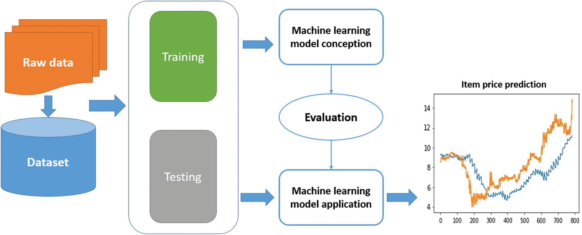
Figure 3: The proposed framework for gift prediction problem
One of the goals of online retailers is to increase the desirability and the value of the products they sell. Offering promotions and special offers is an effective method for driving ancillary traffic to the site. The collected data are real data from an online retailer1; this retailer has launched a special sale of gifts for the Christmas event. The following data described in Tab. 1 are used for building the proposed models. Then, the proposed models can help the online retailer set the prices for their new gifts. The dataset consists of two portions. The first portion includes 20,179 records as the training data, and the second portion includes 13,519 records as the test data.
In Tab. 1, there are 15 input features and one output (i.e., response) feature. The response feature is the gift price, which is given in decimal points. The input features are of varying importance. For instance, the feature gift_id represents a unique ID for each input row. Thus, this feature is dropped from the input feature space of the proposed model, as it is a useless feature.
In the proposed models, we made use of features number 2 to 4, as these three input features capture important information that can be utilized by the proposed model to predict the gift price accurately. For instance, feature number 2 (i.e., gift_type) categorizes the input data into different groups such as clothing and electronics. This feature helps the proposed model predict the gift price with a given price range, as each category of gifts has a different price range. The other two features, features number 3 and 4, define the industry and the category of the gift, which are important features to determine the price range as well.
Features number 5, 6, 13, and 14 are not utilized in the proposed models, as these features are date and time features. In regression problems, the model can handle only numerical data. In addition, considering these four features should change the problem from a regression problem to a time-series analysis problem, the latter is beyond the scope of the current work.
Six features (i.e., lsg_1 to lsg_6) are important features that are camouflaged for the sake of privacy protection of the online retailer providing the data. These features should be used because as described by the data owner, these six features are related to the gifts. Thus, we included these six features in the proposed models. Finally, feature number 15 (is_discounted) is the last input feature. This feature is a Boolean feature that indicates whether the gift price is discounted. To summarize, there are ten utilized input features, namely, gift_type, gift_category, gift_cluster, gift_cluster, and lsg_1 to lsg_6.
4.3 Evaluation Metrics of the Proposed System
One of the most active study areas in machine learning is loss functions. Loss functions are critical in the development of machine learning algorithms and their performance optimization [32]. This section will offer a brief overview of the most often used loss functions in price prediction task, including the Mean Square Error (MSE), the Root Mean Square Error (RMSE), the Mean Absolute Error (MAE), R-squared, and Mean Absolute Percentage Error (MAPE).
The Mean Squared Error (MSE) is a model assessment statistic that is often used in conjunction with regression models. The mean squared error of a model in relation to a test set is equal to the average of the squared prediction errors over all occurrences in the test set. The prediction error is defined as the difference between the actual and predicted values for a certain occurrence [33] as follows:
The Mean Absolute Error (MAE) is a metric for comparing the distinct values of two continuous variables. It is an average/mean of the absolute error that is computed using the saw me scale as the data source. It cannot be used to compare series with varying scales [34].
4.3.3 Root Mean Square Error (RMSE)
The Root Mean Square Error (RMSE) is computed by increasing the residuals by their square root. It represents the design’s outright fit to the information, suggesting how close the observed data points are to the design’s expected worth at the moment. The R-squared value is a relative measure of the fit, while the RMSE value is an absolute value. RMSE might additionally be understood as the standard deviation of the unexplained variance, because it is revealed in the exact same units as the response variable. Lowered RMSE readings indicate a much better match. The root mean square error is a helpful sign of how successfully the design anticipates the reaction [34].
R-squared is a statistic that indicates a model’s quality of fit. It is a statistical measure of how closely the regression line approximates the real data in the context of regression. It is so critical when a statistical model is employed to forecast future events or to evaluate hypotheses. There are other variations (for further information, see the remark below); the one shown here is the most generally used:
The sum squared regression is equal to the sum of the residuals squared, while the total sum of squares is equal to the sum of the data’s deviations from the mean squared. Because it is a percentage, it can only accept values between 0 and 1 [35].
4.3.5 Mean Absolute Percentage Error
Due to its scale independence and interpretability, the mean absolute percentage error (MAPE) is one of the most extensively used metrics of prediction accuracy. Let
where
The proposed models are implemented in the Python programming language. We mainly used the Scikit-learn machine learning library. It is open-source and includes efficient implementations of several machine learning algorithms. In addition, we used pandas and NumPy for data processing. Finally, we used Matplotlib and seaborn packages for the visualization purpose of the data and results. For the statistical model (i.e., ARIMA), we utilized the statsmodels package. Statsmodels is an open-source package with a variety of efficient implementations of many statistical models.
For the data analysis task, we handled the outliers of the dataset by applying the percentile function to find the n-th percentile of the input online retail dataset. Then, we removed the input data with the highest ten percentile and the lowest ten percentile.
We proposed using the default parameters of the utilized machine learning models. The exception to this assumption is the Ridge model. We set the alpha parameter to ridgecv.alpha_value, and we set the normalize parameter to True.
For the statistical model, we applied the grid search technique to find out the best combination of the values of the parameters p, d, and q. The grid search function is considered a brute-force approach to obtain the best prediction accuracy rate based on selecting the best values of the model three parameters.
The experiments were conducted on a computer with an Intel(R) Core(TM) i5-7200U CPU@ 2.50 GHz. The utilized OS is 64-bit Windows 10. All implementations are written in the Python programming language. We used the full dataset of Christmas gifts from an online retailer to train and test the proposed statistical and machine learning models. We used the split 80% and 20% for the training and test data, respectively. All the machine learning models’ parameters are set to the default values of the Scikit-learn package. The ARIMA model parameters
The first point of comparison is the basic evaluation metric scores. We evaluated the proposed model on four different metrics, namely, 1) MAE, 2) RMSE, 3) MAPE, and 4)
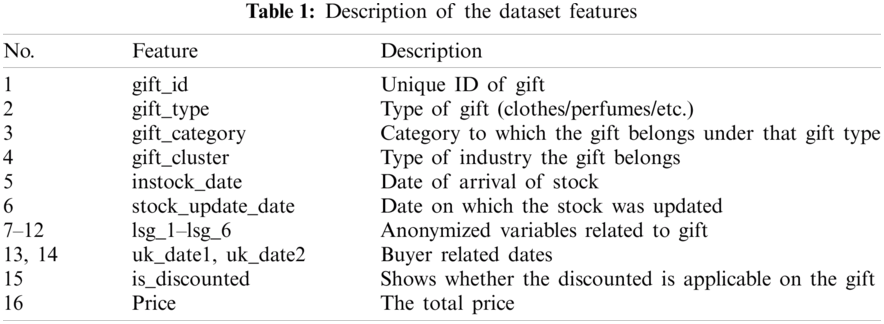
The second point of comparison is the visual results. In Fig. 4, we plotted the actual prices in green and the predicted price by the random forest model in red. The plotted values show the accuracy of the model, as both types of prices are almost identical.
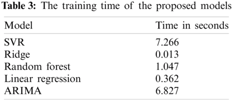
The obtained results outline that the statistical ARIMA model yielded a comparable result to the machine learning-based model. While the best results are produced by the random forest model, the ARIMA model was the second-best model. However, the performance gap between the random forest and ARIMA was not large. Thus, the recommendation of these results is that both machine learning and statistical models are suitable for the task of price prediction for retailer seasonal goods. Tab. 3 lists the times required to train the proposed models in seconds. The training running times of the ridge model is the smallest one, while the SVR model training time is the largest. The random forest model, the one with the best evaluation metric scores, has an average training time of 1 s.
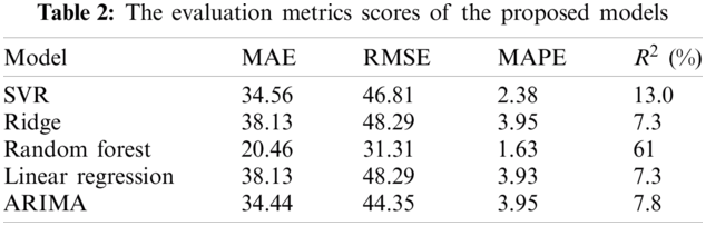
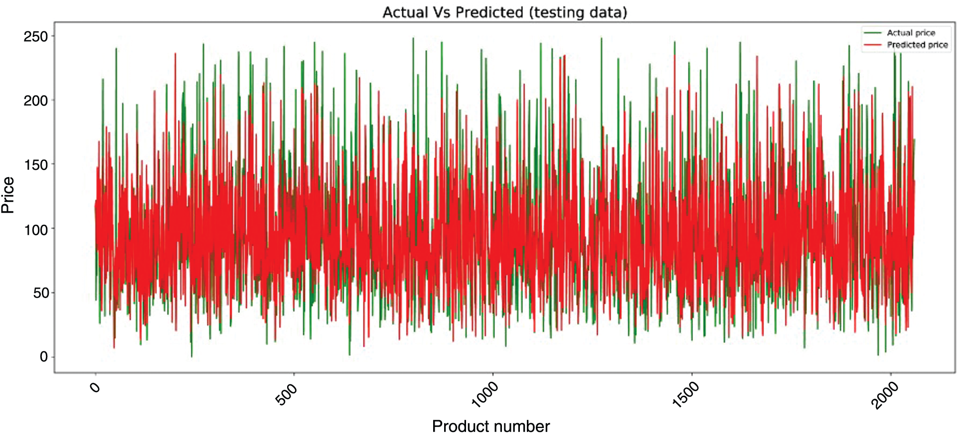
Figure 4: The actual vs. the predicted prices using random forest model
In this work, we studied the task of predicting pricing for retail goods. We focused on predicting the prices of seasonal Christmas items. We employed a real dataset of Christmas gifts from an online retailer. We utilized four machine learning-based models (i.e., SVR, random forest, ridge, linear regression) and one statistical model (ARIMA) to predict the prices of these items. The proposed models are evaluated on four different metrics, namely, MAE, RMSE, MAPE, and
This study recommends the random forest machine learning-based model and the ARIMA statistical-based model to address the problem of predicting seasonal goods’ pricing. The future directions include building hybrid models for the sake of improving the prediction quality. The hybrid models can be achieved using ensemble learning techniques. Moreover, we proposed framing the problem as a time-series problem and to include the date and time input features in the proposed models. For instance, we can utilize the well-known recurrent neural network for predicting the seasonal goods prices as a time series problem.
Funding Statement: The authors received no specific funding for this study.
Conflicts of Interest: The authors declare that they have no conflicts of interest to report regarding the present study.
1https://www.kaggle.com/shashwatwork/christmas-gift-price-prediction
1. Z. Khan, T. Alin and A. Hussain, “Price prediction of share market using artificial neural network ‘ANN’,” International Journal of Computer Applications, vol. 22, no. 2, pp. 42–47, 2011. [Google Scholar]
2. H. Abrishami and V. Varahrami, “Different methods for gas price forecasting,” Cuadernos de Economía, vol. 24, no. 96, pp. 137–144, 2011. [Google Scholar]
3. S. Kamley, S. Jaloree and R. S. Thakur, “Multiple regression: A data mining approach for predicting the stock market trends based on open, close and high price of the month,” International Journal of Computer Science Engineering and Information Technology Research, vol. 3, no. 4, pp. 173–180, 2013. [Google Scholar]
4. W. Sun and C. Huang, “A novel carbon price prediction model combines the secondary decomposition algorithm and the long short-term memory network,” Energy, vol. 207, pp. 1–15, 2020. [Google Scholar]
5. E. Gegic, B. Isakovic, D. Kečo, Z. Mašetić and J. Kevric, “Car price prediction using machine learning techniques,” TEM Journal, vol. 8, no. 1, pp. 113–118, 2019. [Google Scholar]
6. K. Tziridis, T. Kalampokas, G. A. Papakostas and K. I. Diamantaras, “Airfare prices prediction using machine learning techniques,” in European Signal Processing Conf., Kos, Greece, pp. 1036–1039, 2017. [Google Scholar]
7. J. Contreras, R. Espinola, F. J. Nogales and A. J. Conejo, “Arima models to predict next-day electricity prices,” IEEE Transactions on Power Systems, vol. 18, no. 3, pp. 1014–1020, 2003. [Google Scholar]
8. P. F. Pai and C. S. Lin, “A hybrid ARIMA and support vector machines model in stock price forecasting,” Omega, vol. 33, no. 6, pp. 497–505, 2005. [Google Scholar]
9. R. J. Hyndman and G. Athanasopoulos, Forecasting: Principles and practice, 2nd ed., Melbourne, Australia: OTexts, 2018. [Online]. Available: https://otexts.com/fpp2/. [Google Scholar]
10. B. M. Golam and A. F. Lukman, “A new ridge-type estimator for the linear regression model: Simulations and applications,” Scientifica, vol. 2020, pp. 1–16, 2020. [Google Scholar]
11. A. E. Hoerl and R. W. Kennard, “Ridge regression: Biased estimation for nonorthogonal problems,” Technometrics, vol. 12, no. 1, pp. 55–67, 1970. [Google Scholar]
12. J. S. Kidwell and L. H. Brown, “Ridge regression as a technique for analyzing models with multicollinearity,” Journal of Marriage and Family, vol. 44, no. 2, pp. 287–299, 1982. [Google Scholar]
13. A. E. Hoerl, R. W. Kannard and K. F. Baldwin, “Ridge regression: Some simulations,” Communications in Statistics, vol. 4, no. 2, pp. 105–123, 1975. [Google Scholar]
14. M. Awad and R. Khanna, “Support vector regression,” in Efficient Learning Machines. Berkeley, CA, USA: Apress, pp. 67–80, 2015. [Google Scholar]
15. S. F. Crone, J. Guajardo and R. Weber, “A study on the ability of support vector regression and neural networks to forecast basic time series patterns,” in IFIP AI 2006. IFIP International Federation for Information Processing. vol. 217. Berlin, Germany: Springer, pp. 149–158, 2006. [Google Scholar]
16. L. Wang, X. Zhou, X. Zhu and Z. Dong, “Wenshan Guo, estimation of biomass in wheat using random forest regression algorithm and remote sensing data,” Crop Journal, vol. 4, no. 3, pp. 212–219, 2016. [Google Scholar]
17. H. Jang and J. Lee, “An empirical study on modeling and prediction of bitcoin prices with bayesian neural networks based on blockchain information,” IEEE Access, vol. 6, pp. 5427–5437, 2018. [Google Scholar]
18. S. A. Alahmar, “Using machine learning arima to predict the price of cryptocurrencies,” ISeCure The ISC Int’l Journal of Information Security, vol. 11, no. 3, pp. 139–144, 2019. [Google Scholar]
19. N. Garg, K. Soni, T. K. Saxena and S. Maji, “Applications of autoregressive integrated moving average (arima) approach in time-series prediction of traffic noise pollution,” Noise Control Engineering Journal, vol. 63, no. 2, pp. 182–194, 2015. [Google Scholar]
20. Y. Dong, S. Li and X. Gong, “Time series analysis: An application of arima model in stock price forecasting,” in Proc. of the 2017 Int. Conf. on Innovations in Economic Management and Social Science, Hangzhou, China, pp. 703–710, 2017. [Google Scholar]
21. D. T. Phan, “Housing price prediction using machine learning algorithms: The case of Melbourne city, Australia,” in Int. Conf. on Machine Learning and Data Engineering, Sydney, NSW, Australia, pp. 35–42, 2018. [Google Scholar]
22. M. Shastri, S. Roy and M. Mittal, “Stock price prediction using artificial neural model: An application of big data,” EAI Endorsed Transactions on Scalable Information Systems, vol. 6, no. 20, pp. 1–8, 2018. [Google Scholar]
23. M. Su, Z. Zhang, Y. Zhu, D. Zha and W. Wen, “Data driven natural gas spot price prediction models using machine learning methods,” Energies, vol. 12, pp. 9, 2019. [Google Scholar]
24. N. I. Nwulu, “A decision trees approach to oil price prediction,” in Int. Artificial Intelligence and Data Processing Symp., Malatya, Turkey, pp. 1–5, 2017. [Google Scholar]
25. A. Sharma, D. Bhuriya and U. Singh, “Survey of stock market prediction using machine learning approach,” in Int. Conf. of Electronics, Communication and Aerospace Technology, Coimbatore, India, pp. 506–509, 2017. [Google Scholar]
26. M. Vijh, D. Chandola, V. Tikkiwal and A. Kumar, “Stock closing price prediction using machine learning techniques,” Procedia Computer Science, vol. 167, no. 4, pp. 599–606, 2020. [Google Scholar]
27. A. Fathalla, A. Salah, K. Li, K. Li and P. Francesco, “Deep end-to-end learning for price prediction of second-hand items,” Knowledge and Information Systems, vol. 62, no. 12, pp. 4541–4568, 2020. [Google Scholar]
28. M. Ouahilal, M. E. Mohajir, M. Chahhou and B. ELmohajir, “A novel hybrid model based on Hodrick–Prescott filter and support vector regression algorithm for optimizing stock market price prediction,” Journal of Big Data, vol. 4, no. 31, pp. 4148, 2017. [Google Scholar]
29. B. M. Henrique, V. A. Sobreiro and H. Kimura, “Stock price prediction using support vector regression on daily and up to the minute prices,” Journal of Finance and Data Science, vol. 4, no. 3, pp. 183–201, 2018. [Google Scholar]
30. S. McNally, J. Roche and S. Caton, “Predicting the price of bitcoin using machine learning,” in 26th Euromicro Int. Conf. on Parallel, Distributed and Network-Based Processing, Cambridge, UK, pp. 339–343, 2018. [Google Scholar]
31. M. Nikou, G. Mansourfarand and J. Bagherzadeh, “Stock price prediction using DEEP learning algorithm and its comparison with machine learning algorithms,” Intelligent Systems in Accounting, Finance and Management, vol. 26, no. 4, pp. 164–174, 2019. [Google Scholar]
32. Q. Wang, Y. Ma, K. Zhao and Y. Tian, “A Comprehensive survey of loss functions in machine learning,” Annals of Data Science, vol. 7, no. 2, pp. 1–26, 2020. [Google Scholar]
33. J. Rougier, “Ensemble averaging and mean squared error,” Journal of Climate, vol. 29, no. 24, pp. 8865–8870, 2016. [Google Scholar]
34. M. Spüler, A. Sarasola-Sanz, N. Birbaumer, W. Rosenstiel and A. Ramos-Murguialday, “Comparing metrics to evaluate performance of regression methods for decoding of neural signals,” in 37th Annual Int. Conf. of the IEEE Engineering in Medicine and Biology Society, Milan, Italy, pp. 1083–1086, 2015. [Google Scholar]
35. A. Gelman, B. Goodrich, J. Gabry and A. Vehtari, “R-squared for bayesian regression models,” American Statistician, vol. 73, no. 3, pp. 307–309, 2019. [Google Scholar]
36. S. Kim and H. Kim, “A new metric of absolute percentage error for intermittent demand forecasts,” International Journal of Forecasting, vol. 32, no. 3, pp. 669–679, 2016. [Google Scholar]
 | This work is licensed under a Creative Commons Attribution 4.0 International License, which permits unrestricted use, distribution, and reproduction in any medium, provided the original work is properly cited. |