Computers, Materials & Continua DOI:10.32604/cmc.2022.020613
Article

Utilizing the Improved QPSO Algorithm to Build a WSN Monitoring System

Wen-Tsai Sung1 and Sung-Jung Hsiao2,*

1Department of Electrical Engineering, National Chin-Yi University of Technology, Taichung, 411030, Taiwan
2Department of Information Technology, Takming University of Science and Technology, Taipei City, 11451, Taiwan
*Corresponding Author: Sung-Jung Hsiao. Email: sungjung@gs.takming.edu.tw
Received: 31 May 2021; Accepted: 08 July 2021

Abstract: This research uses the improved Quantum Particle Swarm Optimization (QPSO) algorithm to build an Internet of Things (IoT) life comfort monitoring system based on wireless sensing networks. The purpose is to improve the quality of intelligent life. The functions of the system include automatic basketball court lighting system, monitoring of infants’ sleeping posture and accidental falls of the elderly, human thermal comfort measurement and other related life comfort services, etc. On the hardware system of the IoT, this research is based on the latest version of ZigBee 3.0, which uses optical sensors, 3-axis accelerometers, and temperature/humidity sensors in the IoT perception layer. In the network transmission layer, the central network architecture is used for connection. In the application layer, we have designed a graphical interface for real-time values and information that can be read at any time and place using mobile devices. In this study, authors use the improved QPSO algorithm in the calculation part, so that the target can be effectively positioned outside the numerous surveillance data. This study uses various sensor data fusion technologies to make the IoT system becomes able to provide more extensive and even better services than ever before. In short, this research work has proven to be an effective way to reduce power consumption, improve medical quality and provide higher comfort for intelligent lift level.

Keywords: Quantum particle swarm optimization; IoT; wireless sensor network; ZigBee

1  Introduction

The IoT is a network composed of global connected things, which is constantly expanding in scale. The connected things can transmit data and communicate with each other. These objects have unique identification codes and have a wide range of applications, covering fields such as mobile devices, household appliances and automobiles in one fell swoop. Traditionally, the connection capability mainly relied on Wi-Fi wireless networks, but now 5G and other types of network platforms have gradually been able to handle large data sets with the speed and reliability [1–3]. The ultimate goal of IoT devices collecting and transmitting data is to analyze and accelerate the formulation of strategies. This is what AI technology is good at: building AIoT networks with the help of advanced analysis and machine learning [4–5].

The IoT is widely used in network integration through intelligent perception, recognition technology and pervasive computing and other communication perception technologies. Therefore, it is called the third wave of the development of the world's information industry after computers and the Internet [6–7]. This research is based on the huge amount of data calculations and burdens of the IoT. Therefore, an improved quantum particle swarm optimization algorithm with powerful computing capabilities is used to solve this problem. The IoT system in this research uses quantum computing, which can enhance the network. The computing power of the road and the reduction of network delay, and the man-machine interface of the system have artificial intelligence capabilities, timely analysis and prediction of the optimization of life comfort, and increase the data storage capacity and the security of cloud computing [8–9]. Through a wireless network, an IoT covers the linkage among tagged objects for efficient tracking and transparent management. Other than monitoring and anti-theft, a wide variety of IoT applications can be found in the fields of medical treatment, public transportation, services, home use devices, manufacturing, urbanization, etc. Hence, IoT is viewed as a promising technique in further market. A number of simulation experiments are made in this work through a ZigBee network involving RFID technique for recognition and data communication among sensor nodes. Furthermore, an IoT is formed by electrical connection of various types of devices as sensor nodes [10–14].

2  Improved QPSO Algorithms

PSO refers to a swarm intelligence theory-based optimization algorithm under the assumption that there is a swarm of birds foraging randomly for a single piece of food. However, all the birds do not know where the search target, namely the food, is, but merely know the distance between the search target and their current positions. Hence, there is no doubt that the optimal search scope is the neighborhood of the bird nearest to the target. In terminology, a bird is termed as a particle, that is, a potential solution in this optimization problem. Two extremums, the local optimization pbest and the global optimization gbest, are tracked during each iterative search in such a way that the position and the speed of each particle are dynamically updated and the optimization problem is resolved eventually. First proposed by Kennedy et al. [15–16], the particle speed and position in a standard PSO are expressed as:

vi+1=ωvi+ϕ1⋅r1⋅(pbest−xi)+ϕ2⋅r2⋅(gbest−xi)(1)

where ω denotes the inertia weight factor.

xi+1=xi+vi+1(2)

In quantum mechanics, the motion of a particle is represented by a wave function in a Hilbert space, rather than a position vector and a velocity, namely

ψ(x,t)=ψ(x)f(t)(3)

where f(t)=e−iEht and E denotes the state level. Hence, the wave function is a sinusoidal function of time, and, according to de Broglie relationship, the wave function is referred to as a steady-state wave function since the energy level E is deterministic. Hence, the probability density function of locating a particle at the position x is found from a Schrodinger equation as

|ψ(x,t)|2=|ψ(x)|2(4)

In this manner, a particle can be fully described by ψ(x), instead ofψ(x,t), which is rewritten as

ψ(x)=1/Lexp⁡(−‖p−x‖/L)(5)

and the probability density function is expressed as

|ψ(x)|2=1/L⋅exp⁡(−2‖p−x‖/L)(6)

The search scope for a particle is specified by the parameter L(t+1)=2α×|p+x(t)| up to potential energy strength. It is unwise to apply the best position Pi of a particle to the entire population, for the reason that non-uniform convergence rate gives rise to a premature convergence problem in the case of a small population. A mean best position (mbest) is introduced as the centroid of all the particles, namely [17–18],

mbest=∑i=1M⁡pi/M=(∑i=1M⁡pi1/M,∑i=1M⁡pi2/M,…,∑i=1M⁡pid/M)(7)

where M denotes the size of population, Pi the best position of particle i. In this manner, L equals L(t+1)=2β×|mbest−x(t)|, where β represents the contraction expansion coefficient affecting the convergence rate of a single particle and the algorithm performance. Referring to the adaptive changes in the law of inertia weightω in a PSO model, β is defined as

β=βmax−(βmax−βmin)⋅TmaxT(8)

Subsequently, through Monte Carlo simulation of Eq. (7), the position function of a particle is given by x(t)=p±L/2ln⁡(1/u). The substitution of L yields the improved QPSO algorithm in an iterative form as

x(t+1)={p+β×|mbest−x(t)|ln⁡(1/u)(if u<0.5)p−β×|mbest−x(t)|ln⁡(1/u)(if u≥0.5)(9)

where p=(r1⋅pbest+r2⋅gbest)/(r1+r2),r1,r2∈rand(0,1).

The improved QPSO algorithm is stated as follows.

Step 1:   Initialize a quantum particle swarm, and specify the parameters thereof;

Step 2:   Assess the fitness of each particle, and then define a fitness function according to the problem dealt with.

Step 3:   For each particle, the current fitness f(xi) is compared with the record high of fitness f(pbesti), and if f(xi)<f(pbesti),then pbesti=xi. Likewise, compare the current fitnessf(xi) of all the particles with the best fitness f(pbesti), and if f(xi)<f(pbesti),then the global optimization solution is pbesti=xi.

Step 4:   The best position mbest is given as Eq. (7).

Step 5:   The position of a particle is updated as Eq. (9) in a QPSO algorithm, and create a new swarm x(t+1).

Step 6:   The optimization process terminates once the requirements are fulfilled. Otherwise, T=T+1 and skip to step 2 for the next iteration. The process is repeated until the maximum number of iterations is reached or the evaluation value is found below a given accuracy.

A flow chart of an improved QPSO algorithm is exhibited in Fig. 1.

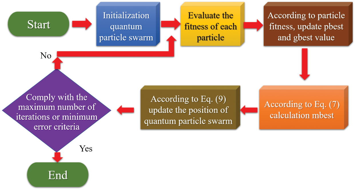
Figure 1: Improved QPSO algorithm flowchart

This system is a WSN intelligent sensor network with a QPSO algorithm based on the IoT architecture. The system can collect the environmental parameters of the sensor in real-time. Then the system sends the environmental parameter values to the back-end database. Through the calculation of the system's QPSO method, the system can analyze and process various environmental conditions, and perform intelligent and efficient environmental control in a timely manner. This is an integrated application of QPSO and artificial intelligence methods. Aiming at the problem of inaccurate selection of weights and thresholds for existing particle swarms, an improved quantum particle swarm optimization algorithm is used to optimize the traditional particle swarm weights and thresholds. First, in the improved quantum particle swarm optimization algorithm, a two-layer multi-group optimization strategy is used to improve the optimization ability of the entire population, and then chaotic reverse learning is used in each subgroup to enhance the optimization ability of the particle swarm. Finally, the improved optimal weights and thresholds of quantum particle swarms are used. The experimental results show that the improved quantum particle swarm optimization algorithm can effectively improve the global optimization ability and convergence of the traditional particle swarm, and make accurate predictions for this research [19–21].

3  System Hardware Architecture

In the hardware architecture of this research, the authors used the one shown in Fig. 2. In this research, the wireless sensor network and sensor technology with the 2.4 GHz CC2530 ZigBee 3.0 development module circuit board that are used to complete a smart life monitoring system is constructed. The system includes related hardware components and devices, such as various sensor components, node signal processing chip modules and antennas, RFID and readers, which belong to the perception layer of the IoT, as for network transmission. The layer uses the ZigBee module to transmit the data in the perception layer to the coordinator, which is the gateway. In the system design of the application layer, the authors use Python programs and design user graphical interfaces to allow end users to make some settings and Operation, its functions include thermal comfort monitoring and environmental lighting control, which can be used in baby care, fall warning for the elderly, smart and comfortable life and other projects [22–23].

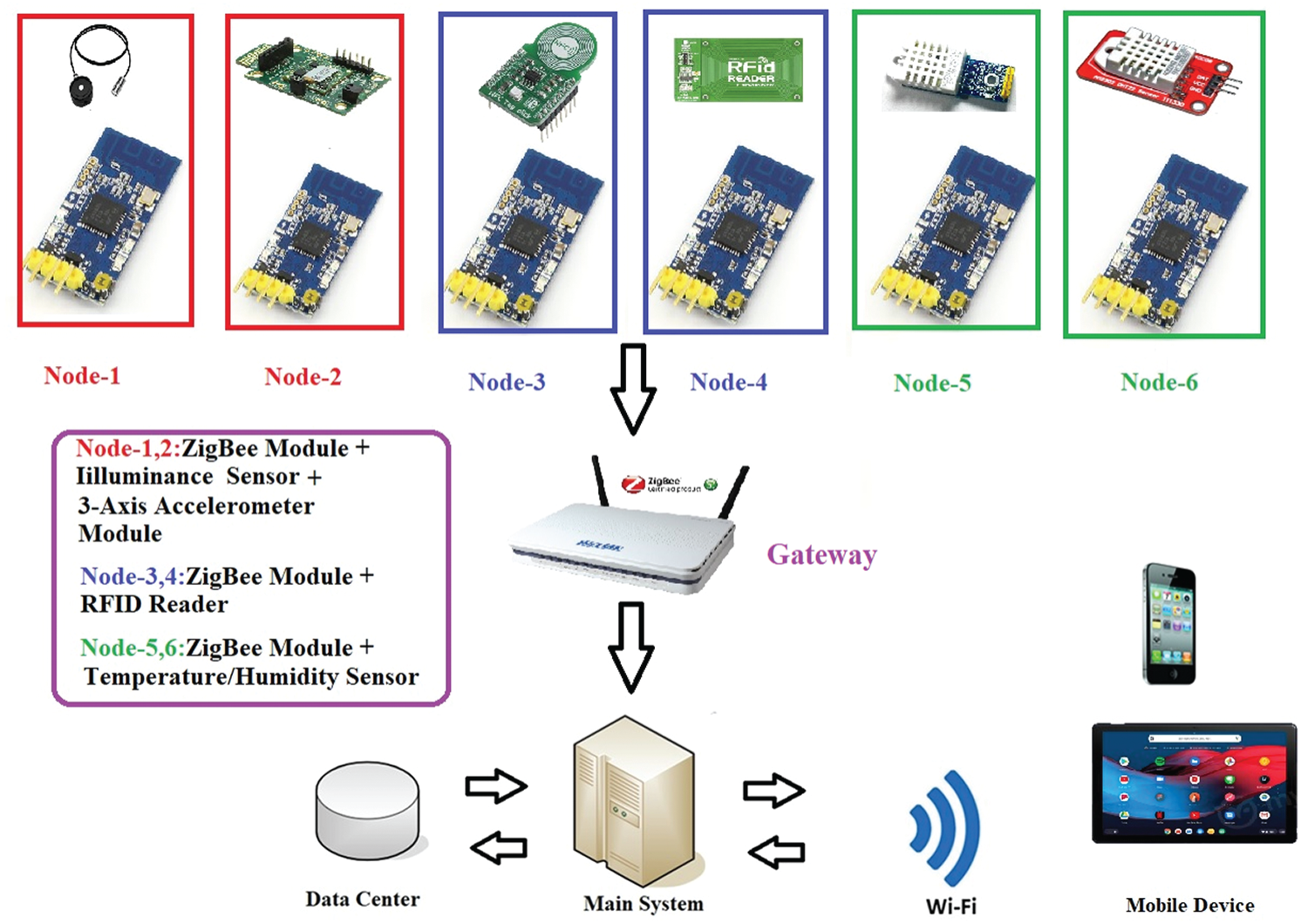
Figure 2: Constituents of the proposed ZigBee-based monitoring system

This system uses the improved quantum particle swarm optimization algorithm to analyze and sense the multiple calculation results and use this calculation result as the judgment of artificial intelligence as the basis for the judgment criterion of artificial intelligence. Data centers promote the development of the cloud. In fact, the so-called cloud computing and cloud computing refer to Internet computing. The network is a connection between the client's personal computer and the remote server through a cable. The data center in this study also refers to the functions of cloud computing and services [24]. ZigBee embedded chip Ti-CC2530 intelligent environment sensing and control nodes mostly use ZigBee wireless sensor network. The CC2530 chip is the SOC chip-CC2530 launched by Texas Instruments (TI) in 2009. This chip is a SOC chip tailored by TI for IEEE802.15.4, ZigBee, ZigBeeRF4CE, and Smart Energy applications. With a large flash memory with a capacity of up to 256KB, CC2530 is suitable for ZigBee PRO applications. In addition, CC2530 combines a fully integrated high-performance RF transceiver, 8051 MCU, and other powerful functions with peripherals, such as built-in ADC, SPI, USB… and other functions, and a SOC chip tailored for energy applications. With a large flash memory with a capacity of up to 256KB, CC2530 is suitable for ZigBee PRO applications. In addition, the CC2530 combines a fully integrated high-performance RF transceiver, 8051 MCU, and other powerful functions and peripherals, such as built-in ADC, SPI, USB… and other functions to facilitate connection with other [25].

4  Lighting Experiment and Analysis

In this study, a photoresist sensor module was used as a light sensor to conduct outdoor lighting simulation experiments. The various experiments in this study have calibration procedures before using the sensor, and the approximate error rate is about ±0.03% or less, which is within the range of the general instrumentation. This is usually used in outdoor environment lighting. For example, the authors achieve the lighting of streets, stadiums and parking lots through light sensor module control circuits. That is, the lighting of the monitored field is controlled, and the data is transmitted through the IoT network layer of this research. The lighting status sensed in the field is transmitted through the ZigBee network node, and finally the terminal displays a long graph and real-time detected data on the screen in the user's graphical interface and stores it in the cloud host.

4.1 Outdoor Lighting Adequate State

In the lighting experiment, we set the lighting range of the outdoor monitored field to be between 85 and 1625 lumens. This setting is in line with the lighting regulations in Taiwan. Fig. 3a shows the real-time values and graphs detected during the current experiment. For most sports fields, this study recommends to use at least 570 Lux, which is 35% of 1625 Lux, and use a yellow indicator light to indicate. When the system detects that the illumination is below 35%, this study suggests that it should be turned on outdoor lighting facilities to provide sufficient illumination. The author uses 35% as the recommended threshold for turning on outdoor lighting equipment.

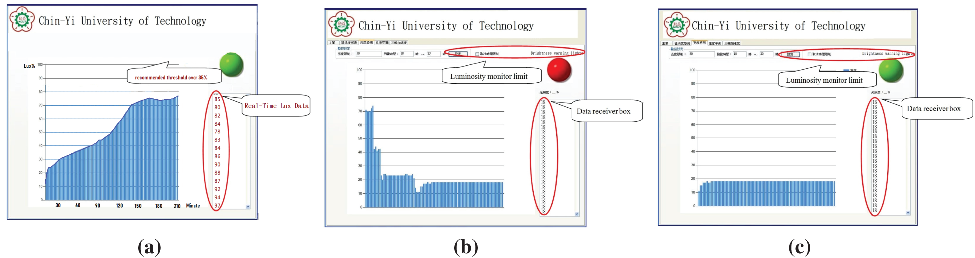
Figure 3: Comparison of lighting in different environments (a) Lighting experiment and analysis (b) An illustration of insufficient outdoor lighting (c) An illustration of a disabled lighting system at night time

4.2 An Illustration of Insufficient Outdoor Lighting

As illustrated in Fig. 3b, a threshold of 30% is specified in a simulation experiment in the case pf an insufficient light level or at night time. In this case, an average illuminance below 20%, far below the threshold, is sensed, transmitted by ZigBee technique to a remote GUI, and the green indicator turns red, according to which the outdoor lighting facility is immediately switched on for illuminance enhancement.

As illustrated in Fig. 3c, the lighting system can be powered on during a specified time span between 18 and 20:00 in case the lighting falls below a threshold of 30%. In other words, at a time point beyond such time slot, the lighting system is deactivated in any case. This feature can be disabled for continuous lighting monitoring.

A smart lighting facility is implemented in the simulation case of a basketball court, achieving the aim of energy consumption reduction in an effective manner. In successive studies, this work together with RFID, easy cards, and so forth, is expected to be applied to pay per use schemes.

5  Infant Take Cares for Experiment and Analysis

In this research, the author designed a nursing simulation experiment with young children and the elderly as monitoring objects. The main sensing element of this experiment is the commonly used three-axis accelerometer module on the market. This experimental design first uses the active RFID tag technology on the tested body to identify the identity, and then installs the accelerometer module on the tested body, and finally can monitor the status of some body changes of the tested body, including the tested body the sleeping position of the person or accidental fall. In the signal transmission part of this experiment, the authors used ZigBee technology to transmit the 3-axis acceleration data to the terminal host, and then displayed the values and corresponding graphics in the user interface immediately, and stored them in the cloud host for future query. Fig. 4a shows some instant messages detected by 3-axis acceleration in the experiment and graphical representations.

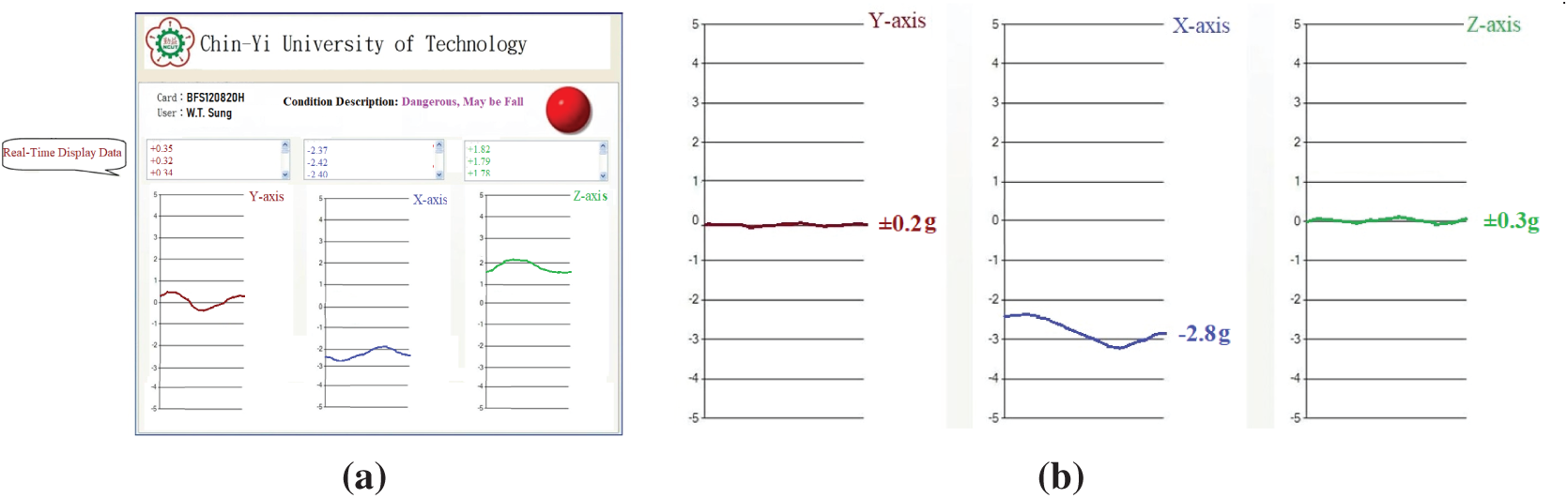
Figure 4: (a) Real-time display of the conditions measured by the 3-axis accelerometer with numerical values and graphs (b) The result of the subject's posture detection state is laying state

5.1 Lying Down State

The main task of this experiment is to detect the changes of the subject's body when lying down. The interval values on the x, y and z axes are displayed as accelerations of ±0.2, −2.8 and ±0.3 g, as shown in Fig. 4b. which the detected condition represents the lying state.

5.2 The Subject Lies Flat on the Left and Right Sides

In this experimental project, Fig. 5 shows that the Z-axis acceleration signal is used to identify the subject is currently lying on the left or right side. The acceleration from 0 g to −2.4 g on the Z axis indicates the difference between the lying state and the left state. The change process is shown in Fig. 5a. If the acceleration signal drops from 0 to +2.6 g, it means the movement from the lying state to the right side, as shown in Fig. 5b.

5.3 Lying State During Sleep

The detection of posture during sleep is very important. It is possible to know the sudden situation of the subject. From the curve comparison chart shown in Fig. 6, we can know the sleep position changes of the tested person. This experiment uses the Z-axis signal to identify. Comparisons the results of this experiment are Figs. 6a and 6b, they can be seen that the z-axis signal changes in the same way. In terms of the x-axis and y-axis signals, their rise and fall indicate that the subject is from the right or turn over to a horizontal front position in the left side lying position.

Figure 5: The detection result of the acceleration signal based on the Z axis when the subject's posture changes (a) The person lays to the left side (b) The person lays to the right side

Figure 6: Accelerometer signal detection comparison chart of posture changes during sleep, the change process of the subject from (a) Left side to (b) Right side to lying down, calculated with three-axis acceleration signals

5.4 Standing Posture Status

Other than the analysis on a lying state, movements, namely an upright standing posture, forward fall, backward fall, rightward fall and leftward fall, are addressed here as well. As illustrated in Fig. 7, a body movement from a lying to a standing state is recognized by a y-axis signal transition from 0 down to −2 g and a z-axis signal transition from 1.5 down to −0.5 g. Both signal tails in the x and y axes represent an upright standing state.

Figure 7: Acceleration signals in an upright standing posture along the x, y and z axes

5.5 Standing Dumping Status

As illustrated in Fig. 8, either a leftward or rightward fall is identified by the x-axis signal. The transition between 0 and 1 g, as exhibited in Fig. 8a, and that between 0 and −1 g, as in Fig. 8b, signify a rightward fall and a leftward fall, respectively.

Figure 8: Acceleration signals in (a) A rightward and (b) A leftward fall along the x, y and z axes

Figure 9: Acceleration signals during (a) A forward and (b) A backward fall along the x, y and z axes

5.6 Standing Forward or Backward Dumping State

As illustrated in Figs. 9a and 9b, either a forward or backward fall is indicated by the y and z-axis signals. The former reflects the falling process, while the latter indicates the falling direction. A signal drop from 0.5 to −0.5 g in Fig. 9a along the z axis represents a forward falling process, while a rise from 0.5 to 1.5 g in Fig. 9b represents a backward falling transition instead.

This monitoring system is applied to medical care systems for both infants and the elderly through a ZigBee network. In case of any urgent matters, a test object is located instantly such that medical stuff can even perform first arid on the test object. Accordingly, the simulation experiment indicates an elevated the quality of medical care.

6  Smart Living Comfort Experiment and Analysis

The purpose of this experiment is to optimize comfort in a smart living environment, so that system users can live in the most comfortable space. In the experiment, we used the SHT10 temperature and humidity sensor module to conduct a simulation experiment. This research refers to the thermal comfort equation dedicated to the Central Meteorological Bureau of Taiwan as shown in Eq. (10) [26]:

CI=T−0.55[1−Exp(d×17.269237.30+d)Exp(T×17.269237.30+T)]×(T−14)(10)

d=T×H100(11)

Among them, CI stands for comfort index, H stands for relative humidity, d stands for dew point, and T stands for temperature in ∘C. Tab. 1 shows that the comfort is divided into 6 levels. The authors use the Python design program to calculate the dew point value and the comfort index. As shown in Fig. 10, the authors gave two examples and calculated the dew point value and comfort index. The case one condition is (T = 30∘C, H = 62%) and case two condition is (T = 25°C , H = 48.6%) [26].

6.1 Environmental Temperature and Humidity Anomalies

Through a Visual Basic-based GUI with an alert indicator, the sensed data are plotted against time and saved as a file. As illustrated in Fig. 11a, a red indicator signifies a temperature beyond 40 or below 20∘C, a need to activate an air conditioner or a radiator. Likewise, as presented in Fig. 11b, a red indicator represents relative humidity beyond 70% or below 50%, a need to turn on a dehumidifier or a humidifier. Furthermore, the rates of change of temperature/humidity are found to have a direct relationship with the comfort level. In short, the GUI is developed as an approach for sensed data collection, presentation and the intended energy consumption reduction [27].

Figure 10: Smart living comfortable

Figure 11: (a) Indication of monitored temperature below or beyond a threshold on a GUI (b) Indication of monitored humidity below or beyond a threshold on a GUI

6.2 Monitoring Experiment and Analysis of Temperature and Humidity in Comfort

6.2.1 Early Stage of the Experiment

This study designed a monitoring experiment of temperature and humidity in comfort. The average outdoor temperature released by Taiwan's Central Meteorological Bureau every hour was used as a reference, and the recommended temperature monitoring system was used to sense indoors. A conclusion can be observed from the comparison curve in Fig. 12 that when the high temperature in the environment drops, the comfort level will be lower. At this time, it is necessary to turn on the air conditioner by the system of this study to achieve the best comfort.

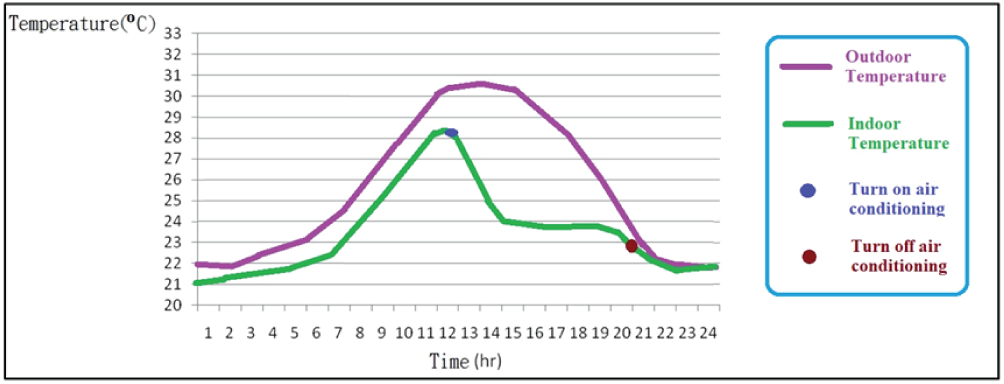
Figure 12: Indoor and outdoor temperature measurement experiment

From this experiment, it can be found that temperature and humidity will affect comfort, especially outdoor humidity is easily affected by weather factors, resulting in a decrease in comfort, and indoor humidity changes have little effect on comfort. Therefore, this study suggests that humidifiers and dehumidifiers can be used. The humidity in the room is adjusted by the machine to optimize comfort. The comparison and adjustment of humidity are shown in Fig. 13.

Figure 13: Indoor and outdoor humidity measurement experiment

6.2.2 Last Stage of the Experiment

The system sets the best comfort index from 19 to 25, and the monitoring time we set focuses on the period from 8:30 in the morning to 5:30 in the afternoon when the average person is in the office. Figs. 15 and 16 compare the results of indoor and outdoor temperature and humidity adjustments. In the experiment, it can be found that after the air conditioner starts to operate at 8:30 in the morning, the indoor temperature and humidity begin to adjust with time, and finally achieve the best comfortable smart living environment.

In this experiment, the authors compared the indoor and outdoor comfort conditions. When the system detects that the comfort level is reduced, the system will recommend turning on the air conditioner to adjust the temperature and humidity to achieve the best indoor comfort environment. When the measured value is low, the system will suggest that you should pay special attention to whether the weather is hot or cold when you go out, so that everyone can be prepared for outdoor activities. The relevant comparison curve is shown in Fig. 14.

Figure 14: Experimental comparison chart: outdoors, comfort index and the best comfort of this study

Figure 15: Flow chart of comfort level evaluation

Figure 16: (a) 500 pieces of temperature data (b) 500 pieces of humidity data (c) 500 pieces of dew point data (d) 500 pieces of comfort level data

7  Improved QPSO Experimental Analysis

A full one-day observation for the ambient temperature/humidity data is made and recorded per 3 s. Up to approximately 25000 pieces of sensed data average out into 500 pieces, this experiment is analyzed by an improved QPSO algorithm that it used Matlab code.

7.1 Comfort Level Computing

To begin with, the respective comfort levels index on 500 pieces of collected data are evaluated with a Matlab program. As illustrated in Fig. 15, the dew point is evaluated as a function of temperature and humidity, the comfort level is then found and rated on a scale of 1 to 6.

Presented in Figs. 16a and 16b are the aforementioned 500 pieces of temperature and humidity data, respectively, while indicated in Figs. 16c and 16d are the evaluated due point and comfort level, respectively.

7.2 Simulation State Analysis

As tabulated in Tab. 2, comfort level is classified into 6 levels, namely, extremely cold, chilly, cool, comfortable, muggy and extremely hot. In Tab. 2, comfort levels of 10, 17.5, 23, 28.5 and 31 are rated as levels 1 (extremely cold), 2 (chilly), 3 (cool), 4 (comfortable), 5 (muggy) and 6 (extremely hot), respectively. A search task for 500 comfort levels, viewed as particles in an improved QPSO algorithm, is performed by a Matlab program. Each particle's speed and position are updated each iteration, until the optimal local solutions and the global solution, i.e., the particle nearest to the specified case, are located.

7.3 Case 4 Simulation State

In this work, a search task is performed through an improved QPSO algorithm on the aforementioned 500 pieces of sensed data. Data 341 is found to best fit level 4. Subsequently, with an error of 3, the portion highlighted in blue represents a comfortable state, as illustrated in Fig. 17.

Figure 17: Data pertaining to case 4

Figure 18: Data pertaining to case 5

7.4 Case 5 Simulation State

Likewise, data 499 is found to best fit level 5. With an error of 1.5, those rated as level 5 are highlighted in blue in Fig. 18. In case of level 5, the muggy state can be eased by use of an air conditioner, a fan, etc. In this simulation experiment, two dominant quantities, i.e., the temperature and humidity, are sensed with a SHT10 temperature humidity sensor module in a ZigBee network. As a comfort measure, the comfort level is evaluated over 500 pieces of collected data. Highlighted in Fig. 17 is the level 4 portion indicating the most comfortable state, while in Fig. 18 is level 5 indicating the muggy state. The analysis does not indicate any uncomfortable cases, namely, Cases 1−2, 3 and 6, which is a validation of this thermal comfort monitoring system.

8  Improved QPSO Algorithm Optimization Analyses

The improved QPSO algorithm is validated by the following 3 typical test functions, and an optimization comparison is made with a basic particle swarm optimization algorithm. Eq. (12) is a sphere function. Eq. (13) shows a peak function and Eq. (14) presents a Shaffer's F6 function. This experiment uses four typical algorithms for optimization experiments. The purpose is to prove that the improved QPSO algorithm proposed by this research is the best and the efficiency is the highest. The author uses Eqs. (12)--(14) three test functions have verified the following algorithms: the first is the basic quantum particle swarm optimization algorithm, the second is the basic particle swarm optimization algorithm, the third is the fuzzy algorithm, and the second is the basic particle swarm optimization algorithm. The four are the improved quantum particle swarm optimization algorithms proposed by this research. Eq. (12) is a Schaeffer's F6 function, Eq. (13) is a number ball function and Eq. (14) is a peak function.

E1(x,y)=0.32+sin2(x2+y2)−0.32[1+0.052⋅(x2+y2)]2(12)

E2(x)=∑i=1n⁡xi2×(n+1)(13)

E3(x,y)=5(1−x)2e−(x+1)2−(y+1)2−8(x3−x2−y4)e−x2−y2−16e−(x+1)3−y2(14)

In this experiment, Tab. 3 is the basic description of the three test equations, in which f3 and f2 are both test minimum problems, and f1 is test maximum problems.

Letting the maximum number of iterations Tmax=100, the particle swarm size n = 10 and the Particle dimension m = 2, a performance measure is defined as

In this experiment, the author set the maximum number of iterationsTmax=350, the number of data items is n = 50 and the particle size m = 5. This experiment defines the error between the expected output value and the actual output value as a performance indicator, such as Eq. (15) shows:

e=1(n+2)∑i=1n⁡(xi−x^i)2×(n+1)(15)

In this experiment, Figs. 19a–19c are the comparison graphs of the calculation results of the four algorithms. Among them, the method proposed by this research is the best, and the others are leading each other. The value in the curve represents the accuracy of the data at the earliest convergence within 350 iterations.

Figure 19: In this experiment, four algorithms (1.QPSO, 2.PSO, 3.Fuzzy, 4.IPSO-this study proposed) are compared with the results of the three equations: (a) Schaffer's f6 functions (b) Spheres (c) Peaks

9  Conclusions and Future Work

This work presents an IoT-based monitoring system by means of a ZigBee wireless sensor network. Using a TI CC2530 development kit, respective smart monitoring systems are built with a light sensor, a 3-axis accelerometer module and a temperature/humidity sensor module mounted on sensing nodes. This smart system is applied to a simulation experiment, namely a basketball court lighting system for demonstration purposes, and extended applications can be found in hospital, household, street, tunnel, parking lot lighting facilities, etc. Hence, this smart monitoring system does as intend achieve the aim of electricity consumption reduction.

This research is designed for the monitoring function of the remote care system. The intended care recipients are infants and young children, the elderly and the sick. If the patient is affected, attach this device to the waist of the care recipient. If the care recipient has an emergency, such as a child in a dangerous sleeping position or an accidental fall of the elderly, the monitoring center will immediately issue an alarm to the medical or security personnel. Crisis management and first aid for care recipients. At present, the global COVID-19 situation is very severe. Many people diagnosed with mild symptoms are promptly accommodated and quarantined because of hospital beds and no rafts. They can only wait at home. The results of this study will be applied to patients’ homes. The surveillance and care system during isolation allows remote medical personnel to grasp the immediate status of patients in real time to reduce the possibility of sudden death. When the results of this research are applied to end-of-care care, it will reduce manpower shortage and improve the quality of medical services. This research uses an improved QPSO algorithm to solve the problem of thermal comfort optimization, and collects many indoor and outdoor temperature/humidity environmental values through the IoT system, which are used as the basis for the adjustment and reference setting of the best comfort of the subsequent smart life.

A greater number of routers are expected to be integrated into a monitoring network, either in a tree or mesh topology, for providing more services. Besides, featuring the measurements of blood pressure, blood glucose concentration, heartbeat, body weight, etc., a health management system is expected to be built for heavily loaded employees. Users can be identified using RFID technique, and automated warning messages as well as reminders can be provided for health concerns.

Acknowledgement: This research was supported by the Department of Electrical Engineering at National Chin-Yi University of Technology. The authors would like to thank the National Chin-Yi University of Technology, Takming University of Science and Technology, Taiwan, for supporting this research.

Funding Statement: The authors received no specific funding for this study.

Conflicts of Interest: The authors declare that they have no conflicts of interest to report regarding the present study.

Availability of Data and Materials: Data sharing not applicable to this article as no datasets were generated or analyzed during the current study.

This work is licensed under a Creative Commons Attribution 4.0 International License, which permits unrestricted use, distribution, and reproduction in any medium, provided the original work is properly cited.