Computers, Materials & Continua DOI:10.32604/cmc.2022.020197
Article

AI Based Traffic Flow Prediction Model for Connected and Autonomous Electric Vehicles

P. Thamizhazhagan1,*, M. Sujatha2, S. Umadevi3, K. Priyadarshini4, Velmurugan Subbiah Parvathy5, Irina V. Pustokhina6 and Denis A. Pustokhin7

1Department of Electrical and Electronics Engineering, University College of Engineering, Panruti, 607106, India
2Department of Electronics and Communication Engineering, Koneru Lakshmaiah Education Foundation, Vijayawada, 522502, India
3Centre for Nanoelectronics and VLSI Design, SENSE, VIT University, Chennai Campus, Chennai, 600127, India
4Department of Electronics and Communication Engineering, K. Ramakrishnan College of Engineering, Tiruchirappalli, 621112, India
5Department of Electronics and Communication Engineering, Kalasalingam Academy of Research and Education, Krishnankoil, 626126, India
6Department of Entrepreneurship and Logistics, Plekhanov Russian University of Economics, Moscow, 117997, Russia
7Department of Logistics, State University of Management, Moscow, 109542, Russia
*Corresponding Author: P. Thamizhazhagan. Email: thamizh@ucep.edu.in
Received: 14 May 2021; Accepted: 15 June 2021

Abstract: There is a paradigm shift happening in automotive industry towards electric vehicles as environment and sustainability issues gained momentum in the recent years among potential users. Connected and Autonomous Electric Vehicle (CAEV) technologies are fascinating the automakers and inducing them to manufacture connected autonomous vehicles with self-driving features such as autopilot and self-parking. Therefore, Traffic Flow Prediction (TFP) is identified as a major issue in CAEV technologies which needs to be addressed with the help of Deep Learning (DL) techniques. In this view, the current research paper presents an artificial intelligence-based parallel autoencoder for TFP, abbreviated as AIPAE-TFP model in CAEV. The presented model involves two major processes namely, feature engineering and TFP. In feature engineering process, there are multiple stages involved such as feature construction, feature selection, and feature extraction. In addition to the above, a Support Vector Data Description (SVDD) model is also used in the filtration of anomaly points and smoothen the raw data. Finally, AIPAE model is applied to determine the predictive values of traffic flow. In order to illustrate the proficiency of the model’s predictive outcomes, a set of simulations was performed and the results were investigated under distinct aspects. The experimentation outcomes verified the effectual performance of the proposed AIPAE-TFP model over other methods.

Keywords: Autonomous electric vehicle; traffic flow predictive; automation industry; connected vehicles; seep learning

1  Introduction

The progressive development of Autonomous Vehicles (AV) in the recent years has attracted the maximum attention from a number of developers working under different applications. Connected AV (CAV) is a standard and new model which is capable of altering the previous transportation systems, thanks to its advanced transmission and sensing abilities, improved travel suitability and its deployment of low-carbon mobility business models [1]. In general, CAVs are electric tools and are effective in the mitigation of carbon production. CA Electric Vehicle (CAEV) is considered to represent a significant portion of the existing revolutions that support low-carbon mobility. In this approach, four main drivers such as automated driving, electric powertrains, system connectivity, and distributed mobility are capable of providing compelling transition towards low-carbon facilities. Hence, one can achieve the simulation outcome in reducing the greenhouse gas (GHG) discharged during transportation. These modifications provide multiple opportunities to reduce carbon production and promising outcomes in terms of sustainability. The basic infrastructure of CAEV is depicted in Fig. 1 [2].

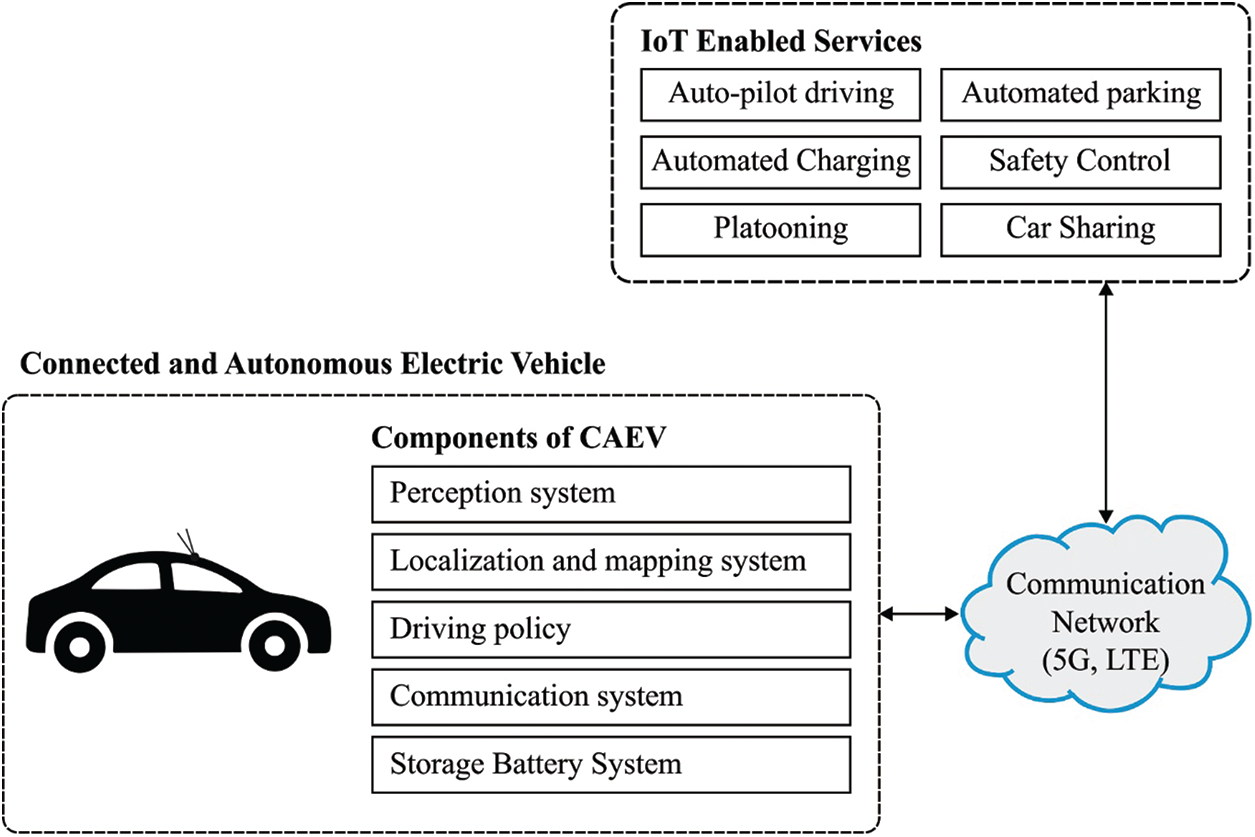
Figure 1: The structure of CAEV model

CAEVs are capable of functioning with maximum vehicle efficacy, when they are charged with power derived from renewable energy sources. This, in turn reduces the emissions and dependency on fossil fuels. Connected Vehicles (CVs), AVs, and Electric Vehicles (EVs), referred altogether as CAEVs, are complex and automated systems [3]. Among these, CV is a vehicle operated by communicating with nearby vehicles, structures, and objects; however, it is neither automatic nor electrically-processed. Secondly, AV is a vehicle which is extensively applied and is suitable for automatic driving without any human contribution. Finally, EV is a type of vehicle operated with available energy preserved in the batteries.

In general, CAEV belongs to EV which is suitable for predicting the environment and directing with or without any human intervention. CAEV detects the environment by applying diverse sensing tools like radar, Light Detection, and Ranging (LiDAR), image sensors, 3D cameras, and so on. Followed by, CAEV is comprised of five major elements. Then, perception system is utilized in the forecasting of atmosphere and relevant objects. Localization and mapping models are deployed in vehicles so that the vehicles are enabled to know the recent location. Driving policy showcases the decision-making ability of CAEV under different scenarios like efficiency negotiation, paving way for vehicles and trespassers, and overtaking transports. In communication network, CAVs are connected with surrounding platforms like vehicle-to-vehicle connectivity (V2V), structure with Vehicle to Infrastructure (V2I) and Internet: Vehicle to anything (V2X), by wireless communication networks. The storage battery is composed of chargers and power banks in the vehicle. Typically, the State of Charge (SoC) level estimates the volume of charge enclosed in a battery.

1.1 Overview of Traffic Flow Prediction (TFP)

Smart models must be developed after taking the improved traffic flow into consideration for traffic flow observation and management. Here, traffic flow is considered to be a degree of vehicles that exceeds specific road segment per unit time based on a reference point. Also, Global Positioning System (GPS) providers such as Google Map predicts the flow of traffic and vehicle speed using Machine Learning (ML) models. To depict this notion in mathematical form, Traffic Flow Prediction (TFP) is assumed as Xti which implies the determined traffic flow value at tth time interval and ith observation. Under the application of applied set Xti, i = 1, 2,…, m and t = 1, 2, 3,…, T, TFP problems are comprised of traffic flow detection from (t + ), which is called a prediction horizon. According to the study conducted earlier [4], TFP is defined as a regression problem, applied in time-series data, from traffic systems. It increases the traffic management by appropriate exploitation and traffic demands on existing road structure. Vehicle route planning, fuel mitigation, and congestion control have been applied in TFP data-based models to collect the previous data flow from different sources (sensors, GPS) and the accumulated data is employed in detection process. Thus, traffic flow data is periodical and the patterns differ from operational days and weekends [5]. Based on the comparison, it is reported that poor climatic condition influences the flow of traffic and results in congestion issues. Various studies have applied shallow TFP models to generate considerable outcomes, while shallow technologies are complex in finding the relations between big data sets. Besides, Deep Learning (DL) is a well-known and reputed model used in traffic prediction and the identification of dependencies in high dimension dataset.

1.2 Deep Learning

In Data Mining (DM) application, DL is an effective approach that initializes the data model through Multi-Layer Perceptron (MLP) structure of human brain [6]. DL resembles the empirical function in a few functions such as image processing, text, audio, and alternate unstructured data. Restricted Boltzmann Machine (RBM) is assumed to be a common method of DL structure. Having been identified with difference from Conventional Neural Network (CNN) approaches, RBM merges with feature learning portion as per the traditional MLP. Feature learning portion mimics the performance of human brain and classifies the data signals. Further, a certain process is used in the enhancement of partial connection of convolution layer as well as dimension layer, prior to Fully Connected (FC) network layer [7]. Thus, the classical shallow NN projections have evolved from feature mapping while the characters are randomly selected. RBM projections are initialized from signal to feature and then to the value. Thus, the data features are freely selected by the system.

1.3 Paper Contribution

The contribution of the paper is stated herewith. The current research paper introduces a novel artificial intelligence-based parallel autoencoder for TFP abbreviated as AIPAE-TFP model in CAEV. The presented model comprises of two distinct procedures namely, feature engineering and TFP. Feature engineering process incorporates few steps such as feature construction, feature selection, and feature extraction. Moreover, Support Vector Data Description (SVDD) model is utilized to filter the anomaly points and smoothen the raw data. At last, AIPAE model is applied in the determination of predictive values of traffic flow. To demonstrate the outcomes of TFP process, a brief simulation analysis was conducted and the results were determined under different metrics.

2  Literature Review

In order to have an appropriate working model for AV, there is a large number of studies required in addition to planning, and cooperation of tasks. This together results in the generation of numerous processing models for task implementation. For example, the AVs are placed in dynamic and ever-changing atmosphere. Multiple approaches [8,9] are used in the implementation of localization process. Path planning mechanism [10] parameterizes the motion primitives and optimizes them into non-linear programming mechanisms. The developers in the literature [11] made use of neural inverse Reinforcement Learning (RL) to direct the AV. In the study conducted by Levin [12], navigation is considered as an optimal management issue since it attempts to overcome the problems based on the distance travelled while generating the path of AV with optimization-related attributes. In this scenario, the parking issues have been addressed in different studies using numerous models [13] that conclude the solution for parking in an accurate location that consumes the maximum time. When AVs are applied in common transportation, the scheduling, routing, and admission management technologies are applied in order to ensure appropriate decision-making and manage the traffic flow to eliminate congestion in a cost-effective manner. A linear program was applied in resolving the scheduling issues [14] and admission control problem depending on Genetic Algorithm (GA). Followed by, the researchers in the literature [15] applied the family module to schedule AV fleets. The study conducted earlier [16] employed game theory models in decision making and congestion elimination processes.

Parametric methods are used to identify traffic flow time series. Some of the models are as follows; Auto Regressive scheme (AR), AR Moving Average (ARMA), Support Vector Regression machine (SVR), AR Integrated Moving Average (ARIMA), and so forth. Among these, AR is utilized in the computation of traffic flow prediction [17]. ARIMA is applied in traffic flow analysis based on periodic difference [18]. Based on SVR, a two-cycle time series of short-term traffic flow predictive methods is presented [19]. A unified AR method, with alternate prediction schemes, is presented in the improvement of prediction function [20]. Thus, parametric schemes are employed in certain traffic data conditions whereas a change in climatic condition affects the accuracy of prediction process. Nonparametric frameworks are employed in big data training and the model structure is computed with no model parameters. Moreover, NN is defined as a typical approach in nonparametric framework. NNs are defined as numerical approaches that enable shared data processing and reflect the behavioral features of animal NN. It is applied extensively in the prediction of traffic flow.

Chokshi et al. [21] relied on NNs to estimate the flow of traffic in urban region in the study conducted earlier. Based on the NN model, Artificial Neural Network (ANN) scheme was used for prediction and management of traffic flow. A prediction mechanism was presented as a combination of ANN and Root-Mean-Square Error (RMSE) method. Additionally, Back Propagation (BP) NN applies the error BP model to train the multilayer feedforward information. In this study, the model prediction accuracy was maximum than NNs and ANN. It used Radial Basis Function (RBF) technology to analyze the chaotic features in the prediction of traffic flow.

In the literature [22], a TFP model was presented for urban roadways based on Long Short Term Memory (LSTM) and sparse autoencoder (SAE). The hybrid TFP model performed well on non-linear traffic flow data and efficiently enhanced the predictive accuracy. Further, the model also offered a multi-scale perspective for transportation and traffic forecasting. In the study conducted earlier [23], a new parallel auto-encoder framework (Para-AF) was presented for Structural Health Monitoring (SHM). The presented Para-AF model distinctly processed the frequency signals and mode shapes for feature selection using dimension reduction. Then, the model integrated the features together in relationship learning for regression. In current study, a novel TFP model for CAEV, inspired from the studies conducted earlier [22,23] is presented. Though the existing works have focused on TFP, there is a need still exists to improve the performance and reduce the computation time. Therefore, in the present work, SVDD model is utilized in the filtration of anomaly points and smoothen the raw data. In addition, AIPAE model is applied to determine the predictive values of traffic flow.

3  The Proposed Traffic Flow Prediction Model for CAEV

The overall working principle of the presented AIPAE-TFP model is shown in Fig. 2. As depicted, the input data undergoes filtration of anomaly data points using SVDD model and the actual data is smoothened with the help of difference-based stationary. Followed by, the AIPAE model is applied in efficient prediction of traffic flow.

3.1 Feature Engineering Process

Construction, selection, and extraction of features are the three major phases of feature engineering process. Initially, feature construction is defined as a process in which the required features are extracted from complicated and actual datasets. It is essential to monitor the distribution and features of actual dataset, and select a reliable way to convert the actual data as accessible features. In case of feature construction, a rule is established for selecting the type of road sections in complete road networks [22]. As a consequence, a selection strategy is deployed for the main road section. Initially, the separation point is removed from road networks. Followed by, the isolation point is placed either at top or bottom of the roads.

Further, it is not applicable to connect with one another since it implies a limited impact on road system. Besides, the connection points from the road network are removed. The junction of a city is highly complex with the inclusion of flyovers, roundabouts, and so on. Additionally, the junctions are highly prone to traffic management restrictions, for instance, speed limitations, where the general features are not represented on road. Finally, the data derived from different sources are unified whereas one-way road section has several lanes with numerous sensors; all these data are concatenated together which results in the reduction of voluminous data [22].

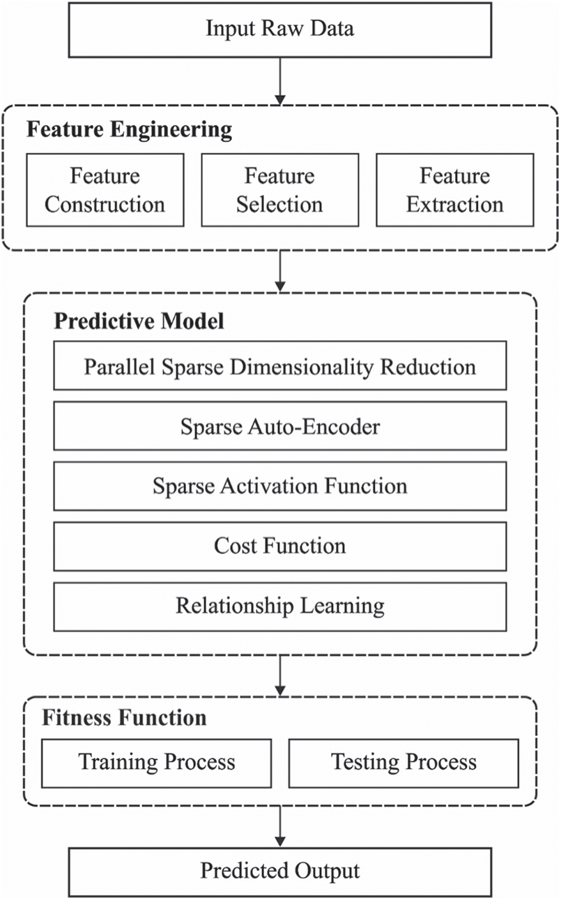
Figure 2: The block diagram of AIPAE-TFP model

Here, the main aim of FS is to extract anomalous features. Then, SVDD is presented with isolation forest approach to identify the anomalous points. SVDD is one of the occasional classifiers that applies high-dimensional hypersphere in the classification of boundary over data sample and prominently reduces the boundary till finding the unwanted points. Hence, the objective function can be determined as given herewith.

Minf(R,a,ξi)=R2+C∑i=1Nξi, (1)

s.t. (xi−a)T(xi−a)≤R2+ξiξi≥0, (2)

where a implies the intermediate point of a sample, depicts the radius from boundary of middle point. C and F illustrate the regularized bias and loss functions. Basically, Lagrange operator is applied to convert the problem into a dual problem and is resolved with the help of kernel function as well as convex optimization model. Here, nonlinear kernel function RBF is depicted as follows

y=e(x−μ)22σ2, (3)

μ and σ imply the expectation and variance, correspondingly. The flow of anomalous prediction is defined in the following points:

1.    Based on the size of data sample, the outliers groups are fixed i.e., outliers_fraction = {o1,…,on}, where n indicates the count of parameter groups.

2.    Apply SVDD and isolation forest methodologies to predict the unwanted points.

3.    Predict the anomalous points using determined outliers_ fraction.

4.    Extract the abnormal points.

Feature extraction decides to identify the best sub-distribution of sample data set by few processes such as coordinate axis conversion, dimension conversion, and so on. In periodic time series prediction domains, difference-based stationary is developed to smoothen the original data. Then, the first-order difference is considered as a sample as given herewith.

Δf(xk)=f(xk+1)−f(xk) (4)

A novel data set is deployed by difference. An accurate difference provides the time intervals applied for training the DL method, which enhances the function of model. Based on the survey, Augmented Dickey-Fuller (ADF) test samples the empty hypothesis, as the unit root is projected in time series sample.

3.2 Traffic Flow Prediction Process

Traditional sequential models (AutoDNet and Sparse Activation Function (SAF)) that facilitates the model shapes and frequencies are often identified as different from the usual ones. Thus, the modal information is isolated as multiple subsets depending on physical value and magnitude scale which are induced for newly-developed system [23].

To predict the damage or failure in the proposed method, two main components are applied and are defined in the following section.

Dimensionality reduction component is used for:

i) The extraction of scale-invariant, associated, and noise-robust features so as to reduce the modal data

ii) The extraction of scale-invariant, associated, and noise-robust features in order to reduce the frequency data;

Relationship learning component is applied in

iii) Learning about the relationship between extracted features and the simulation result

3.2.1 Parallel Sparse Dimensionality Reduction

The key objective of this module is to compute the predefined processes along with dimensionality reduction from the actual input. Hence, the raw input is classified into numerous subsets as given below:

Natural frequencies:q¯r=[q1r,q2r,…,qir]T (5)

Mode shapes:m¯q1r=[m1q1r…mjq1r]T,…,m¯qir=[m1qir…mjqir]T (6)

where q¯r denotes the natural frequencies input subset, qir indicates the ith (i=1,…,n) frequency in rth sample and m¯qir refers to mode shape variables subset that corresponds to ith frequency. A mode shape subset is composed of j count of parameters. Next, the function c¯orir is applied to represent actual input vector in generic development.

Every subset of input data is induced within Stacked Sparse Auto-Encoder (SSAE) method along with Deep Neural Network (DNN) structure so as to reduce the dimension simultaneously. In the newly-developed parallel structure, 1st hidden layer of SSAE learns the local distribution from input subset. The encoding layers of stacked deep AE are applied in dimensionality reduction as shown in Fig. 3 [23]. Based on the problem complexity, ‘deep architecture’ is expanded to match the problem complexity.

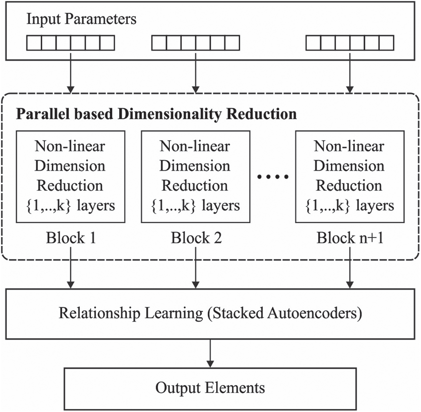
Figure 3: The structure of AIPAE model

3.2.2 Sparse Auto-Encoder

AE model is trained to redevelop the input into output. However, when AE is applied to copy the input to output, it becomes unfit for feature extraction. Further, SAE is an extended version of AE in which the training condition is contributed in sparsity penalty term, on hidden neurons that have evolved from sparse coding, in conjunction with reconstruction error. Since AE regularization is sparse, it has to respond the exclusive statistical features of training dataset. Instead, it is considered as an identity function. Therefore, the purpose of training SAE is to extract the useful features.

A brief deployment of sparsity penalty term is discussed herewith. Assume aj(x(i)) as the activation of hidden neuron j if a network is provided as ith input x(i). Next, the activation of hidden neuron j is averaged across completely-trained datasets:

ρ^j=1m∑i=1m[aj(x(i))] (7)

where m defines the count of samples and is expressed as [23]:

ρ^j≈ρ (8)

where ρ refers to a sparsity attribute which requires pre-defined measurement as small value. Here, the average activation of a hidden neuron j is 0. Moreover, the hidden neurons are often ‘inactive’. This can be accomplished with the help of additional penalty term for optimization objective function, which penalizes ρ^j, when the derivatives are obtained from ρ as given below:

KL(ρ∣∣ρ^j)=ρlogρρ^j+(1−ρ)log(1−ρ)(1−ρ^j) (9)

where KL(·) indicates the Kullback–Leibler (KL) divergence: a value of similarity from two distributions ρ and ρ^j. Besides, the ρ^j diverges from ρ whereas KL divergence gets enhanced monotonically. Therefore, the sparsity penalty term is depicted as provided herewith.

Jsparse(W,b¯)=∑j=1rKL(ρ∣∣ρ^j) (10)

where r refers to the count of neurons in hidden layer and index j is summarized in hidden neurons from the system.

3.2.3 SAF and Cost Function

In SAF process, SAE is applied to decrease the computing dimensionality by learning a sparse depiction of modal data. This can be accomplished in hidden representations. Rectified Linear Unit (ReLUs), otherwise called as encoder activation function, is used across the alternative non-sparse activation functions. In this manner, ReLU controls the sparsity indirectly through model representation. From the newly developed approach, SAE is employed and dimensionality reduction component explores the merits of this approach in comparison with SAF. Hence, the reconstruction cost function of pth layer is calculated as given herewith [23].

Jcostp(W,b¯)=JMSEp(W,b¯)+λJweightp(W,b¯)++βJsparsep(W,b¯) (11)

where

JMSEp(W,b¯)=∑τ=1N‖h¯p−1r−gp(fp(h¯p−1r))‖22 (12)

Jweightp(W,b¯)=12∑l=pp∑i=1sl∑j=1sl+1(wji(l))2 (13)

Eq. (11) implies the overall cost function with Mean Squared Error (MSE) loss term as well as weight decay regularization term. Here, W implies the weight matrix and b denotes the bias vector. The optimization of W and b is carried out using MSE as a loss function in Eq. (12), where p={1,...,k} with k is assumed to be the count of hidden layers in dimensionality reduction, N depicts the overall count of training samples, fp signifies the encoder process for pth layer in which ReLU is applied to impose the sparsity on hidden representation. But, the usage of strong sparsity affects the performance, as it limits the efficiency of the model. Thus, a sparse regularization term is illustrated in Eq. (10) and is included in Eq. (11). Here, β denotes the hyper-parameter that manages the trade-off from reconstruction loss and use the constraints on solution. gp refers to the decoder process for pth layer and fix it as linear activation function g(x)=x to reconstruct the real values of input to output. Further, h¯p−1r represents the compressed hidden feature vector considered from (p−1)th layer from rth sample with h¯0r=c¯orir . Eq. (13) defines a L2-weight decay regularization term, in which wjil illustrates the element in weight matrix W and sl mimics the count of hidden neurons in layer l. In Eq. (11) a hyper-parameter λ is applied to penalize the weight decay term. The unsupervised layer-wise pre-training, relied on SAE, is computed for every layer simultaneously. The sparse hidden illustration of pre-trained AE is assumed as the input for upcoming layer. Consequently, the features derived from kth layer of a block is combined as a novel input vector c¯newr and is injected into nonlinear relationship learning element.

4  Experimental Validation

4.1 Result Analysis

The current section validates the predictive performance of the presented AIPAE-TFP model in terms of precision, recall, and accuracy. The parameter setting, used in the study, is as follows; batch size: 128, learning rate: 0.001, epoch count: 500, and momentum: 0.2. In addition, the prediction results were analyzed under varying volumes and speed indexes. Tab. 1 portrays the predictive results of AIPAE-TFP model in terms of precision under different volumes and speed indexes. The table values portray that the AIPAE-TFP model accomplished the maximum output whereas the SVM model secured the minimum output. At the same time, though few other models such as LSTM, Bi-LSTM, and DBN produced manageable outcomes, the values were not higher than the proposed AIPAE-TFP model.

When examining the precision value on volume index for 5 min, the AIPAE-TFP model achieved a high precision of 0.899, whereas the SVM, LSTM, Bi-LSTM, and DBN models achieved low precision values such as 0.829, 0.831, 0.837, and 0.848 respectively. In case of 25 min time, the AIPAE-TFP model accomplished an effective precision of 0.981, whereas the SVM, LSTM, Bi-LSTM, and DBN models achieved ineffective precision values such as 0.923, 0.923, 0.933, and 0.938 respectively. On the other hand, during the investigation of precision value under 5 min speed index, the AIPAE-TFP model produced a significant precision of 0.953, whereas the SVM, LSTM, Bi-LSTM, and DBN models achieved low precision values such as 0.931, 0.930, 0.940, and 0.944 respectively. Likewise, for 25 min, the AIPAE-TFP model gained a considerable precision of 0.987, whereas the other models such as SVM, LSTM, Bi-LSTM, and DBN models accomplished unsuccessful precision values such as 0.957, 0.952, 0.959, and 0.974 respectively.

Tab. 2 implies the predictive results for AIPAE-TFP model by means of recall under volume and speed indexes. The table values depict that the AIPAE-TFP model produced a maximum output whereas the SVM model exhibited the least output. At the same time, though the LSTM, Bi-LSTM, and DBN models offered manageable results, the values were not higher than AIPAE-TFP model. When examining the recall value on volume index for 5 min, the AIPAE-TFP method reached a high recall of 0.942, whereas the SVM, LSTM, Bi-LSTM, and DBN models accomplished the least recall values such as 0.828, 0.834, 0.833, and 0.846 respectively. Likewise, in case of 25 min, the AIPAE-TFP model accomplished an effective recall of 0.982, while the other methods such as SVM, LSTM, Bi-LSTM, and DBN attained ineffective recall values such as 0.916, 0.928, 0.964, and 0.964 respectively. In this scenario, when examining the recall value under the speed index of 5 min, the AIPAE-TFP model produced a significant recall of 0.954 whereas the SVM, LSTM, Bi-LSTM, and DBN models achieved low recall values such as 0.921, 0.934, 0.944, and 0.957 correspondingly. Likewise, under the existence of 25 min, the AIPAE-TFP model gained a considerable recall of 0.988 whereas the SVM, LSTM, Bi-LSTM, and DBN methodologies produced unsuccessful recall values such as 0.952, 0.955, 0.965, and 0.972 respectively.

Tab. 3 illustrates the prediction outcomes of AIPAE-TFP model with respect to accuracy under volume and speed indexes. The table values depict that the AIPAE-TFP model demonstrated the maximum output whereas the SVM model produced a minimum output. At the same time, though the LSTM, Bi-LSTM, and DBN models offered considerable outcomes, the values were not higher than AIPAE-TFP model. When analyzing the accuracy on volume index for 5 min, the AIPAE-TFP model reached a maximum accuracy of 0.921, whereas the SVM, LSTM, Bi-LSTM, and DBN models achieved the minimum accuracy values such as 0.825, 0.835, 0.834, and 0.844 correspondingly. In line with these, under the application of 25 min, the AIPAE-TFP model accomplished an effective accuracy of 0.983, whereas the SVM, LSTM, Bi-LSTM, and DBN methodologies produced ineffective accuracy values such as 0.915, 0.928, 0.930, and 0.938 respectively. Besides, at the time of investigating the accuracy value under the speed index of 5 min, the AIPAE-TFP model resulted in a significant accuracy of 0.958, while the other models such as SVM, LSTM, Bi-LSTM, and DBN models achieved the least accuracy values such as 0.926, 0.928, 0.937, and 0.946 correspondingly. Likewise, under the presence of 25 min, the AIPAE-TFP model accomplished a considerable accuracy of 0.989 whereas the SVM, LSTM, Bi-LSTM, and DBN models attained inferior accuracy values such as 0.953, 0.951, 0.956, and 0.970 respectively.

Tab. 4 and Fig. 4 shows the results for the average analysis of different TFP models. The results portray that the SVM model exhibited the lowest predictive outcome with an average precision of 0.915, recall of 0.908, and accuracy of 0.910. Followed by, the LSTM model achieved a slightly improved outcome over SVM with an average precision of 0.914, recall of 0.920, and accuracy of 0.914. In line with these, the Bi-LSTM model certainly increased its performance with an average precision of 0.923, recall of 0.928, and accuracy of 0.920. Moreover, the DBN model resulted in a competitive performance with an average precision of 0.932, recall of 0.936, and accuracy of 0.930. At last, the proposed AIPAE-TFP model accomplished a superior predictive outcome with an average precision of 0.957, recall of 0.966, and accuracy of 0.962. From the detailed evaluation results, it can be inferred that the proposed AIPAE-TFP model performs well as it showcased better results under distinct aspects.

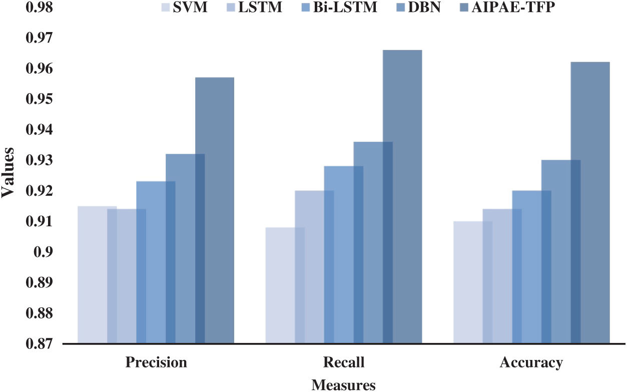
Figure 4: Average result analysis of AIPAE-TFP model

4.2 Discussion

Tab. 5 illustrates the prediction outcomes of AIPAE-TFP model with respect to Computation Time (CT) under volume and speed indexes. The table values depict that the AIPAE-TFP model demonstrated the least output whereas the SVM model accomplished the highest output. Though the LSTM, Bi-LSTM, and DBN models offered considerable outcomes, the values were not lesser than the AIPAE-TFP model. When analyzing the CT value on volume index for 5 min, the AIPAE-TFP model reached a minimum CT of 8.21 m whereas the SVM, LSTM, Bi-LSTM, and DBN models achieved high CT values such as 8.93, 8.42, 8.31, and 8.29 m correspondingly. In line with this, under the application of 25 min, the AIPAE-TFP model accomplished a minimum CT of 9.15 m, whereas the SVM, LSTM, Bi-LSTM, and DBN methodologies achieved ineffective CT values of 9.75, 9.32, 9.27, and 9.21 m respectively. Besides, during the investigation of CT value under the speed index with 5 min, the AIPAE-TFP model produced a significant CT of 9.23 m, while the SVM, LSTM, Bi-LSTM, and DBN models accomplished the least CT values such as 9.47, 9.38, 9.34, and 9.28 m correspondingly. Likewise, under the presence of 25 min, the AIPAE-TFP model gained a considerable CT of 9.49 m whereas the SVM, LSTM, Bi-LSTM, and DBN models attained inferior CT values such as 99.81, 9.68, 9.53, and 9.50 m respectively.

5  Conclusion

The current research article designed an effective AIPAE-TFP model in CAEV to assist in real-time decision making process. The presented model comprises of two distinct procedures namely, feature engineering and TFP. Feature engineering process incorporates few stages such as feature construction, feature selection, and feature extraction. On the other hand, the input data is filtered for anomaly data points using SVDD model and the actual data is smoothened using difference-based stationary. Lastly, the AIPAE model is applied in determining the predictive values of traffic flow. In order to demonstrate the outcome of the TFP process, a brief simulation analysis was conducted and the results were determined under different aspects. The evaluation outcomes verified the effectual performance of the proposed AIPAE-TFP model over other methods. As a part of future work, the AIPAE-TFP model can be incorporated in designing the decision-making model for charging stations.

Funding Statement: The authors received no specific funding for this study.

Conflicts of Interest: The authors declare that they have no conflicts of interest to report regarding the present study.

This work is licensed under a Creative Commons Attribution 4.0 International License, which permits unrestricted use, distribution, and reproduction in any medium, provided the original work is properly cited.