Computers, Materials & Continua DOI:10.32604/cmc.2022.020112
Article

Treatment of Polio Delayed Epidemic Model via Computer Simulations

Muhammad Naveed1,*, Dumitru Baleanu2,3, Ali Raza4, Muhammad Rafiq5 and Atif Hassan Soori1

1Department of Mathematics, Air University Islamabad, Pakistan
2Department of Mathematics, Cankaya University, 06530, Balgat, Ankara, Turkey
3Department of Medical Research, China Medical University, Taichung, 40402, Taiwan
4Department of Mathematics, National College of Business Administration and Economics Lahore, Pakistan
5Department of Mathematics, Faculty of Sciences, University of Central Punjab, Lahore, Pakistan
*Corresponding Author: Muhammad Naveed. Email: nvdm4u@gmail.com
Received: 10 May 2021; Accepted: 27 June 2021

Abstract: Through the study, the nonlinear delayed modelling has vital significance in the different field of allied sciences like computational biology, computational chemistry, computational physics, computational economics and many more. Polio is a contagious viral illness that in its most severe form causes nerve injury leading to paralysis, difficulty breathing and sometimes death. In recent years, developing regions like Asia, Africa and sub-continents facing a dreadful situation of poliovirus. That is the reason we focus on the treatment of the polio epidemic model with different delay strategies in this article. Polio delayed epidemic model is categorized into four compartments like susceptible, exposed, infective and vaccinated classes. The equilibria, positivity, boundedness, and reproduction number are investigated. Also, the sensitivity of the parameters is analyzed. Well, known results like the Routh Hurwitz criterion and Lyapunov function stabilities are investigated for polio delayed epidemic model in the sense of local and global respectively. Furthermore, the computer simulations are presented with different traditions in the support of the analytical analysis of the polio delayed epidemic model.

Keywords: Polio disease; delayed model; stability analysis; computer simulations

1  Introduction

Poliomyelitis is a disease which is most commonly known as Polio, this virus comes from the family of Picornaviridae. Polio is an extremely contagious disease that can incapacitate a person and can be a life-threatening disease. It’s a type of virus that can affect a person at any age but most victims are children who fall under the age of three. This virus feast through the mouth and attacks the nervous system of a person, instigating irreversible paralysis within no time. The initial symptom includes vomiting, headache, fever, fatigue, limb pain, and stiff neck. Poliovirus has three wild types (WPV)-known as type 1, type 2 and type 3. Among these three types, type 1 (WPV1) is still circulating causing permanent paralysis to the victims in Pakistan, Afghanistan and Nigeria. The best defence against this disease is Polio Vaccine which can protect people from getting infected. The usage of these vaccines is prone to its cost as Oral Poliovirus Vaccine (OPV) is economical as compared to Inactivated Poliovirus Vaccine (IPV), it multiplies in the gut of the legatee of exorbitant paramount intestinal immunity than IPV thus more worthwhile in preventing the wild virus from refraining Mission. Recently, due to its serious consequences, significant consideration has been made to observing the vaccine-derived poliovirus (VDPV). Due to the silence and frequent circulation of the vaccine-derived poliovirus (VDPV), poliovirus (PV) surveillance is one of the problematic situations with poor vaccination coverage. Regardless of the aforementioned continual intestinal and ridiculous exceptions, VDPV is natively unstable and can reappear to wild-type wireless according to several research and studies, the vaccine can inflict vaccine-associated flaccid tetraplegia. Substantially, it can produce long-term replicas in conjunction with suboptimal vaccinations. The reciprocity of PV and CD155 receptors accelerate its penetration. After that, the viral RNA is emancipated. The host cell translates the genome attached to the viral particle; it is used as mRNA. For about 20 years, there are no reported cases of Serotype2 wild poliovirus in the world. The last documented case attendant was in 1999 with the naturally happening of serotype (WPV2), with a certificate of global extinction in 2015. For stereotype 3 virus (WPV3), the last reported case was documented in 2012. In April 2016, GPEI executed a globally compatible switch with the trivial poliovirus vaccine. The polio vaccine will not be passed indefinitely in the post-vaccination period. The committee has made a significant difference in our understanding of the strain transfer of oral polio vaccines and their ability to survive in populations with low immunity. As the global polio eradication initiative (GPEI) moves towards the obliteration of the ferocious poliovirus, civil and worldwide health leaders should motionless actively appraise options for supervising the menace of the poliovirus, additionally the use of oral polio vaccine [1]. Elimination of all cases of poliomyelitis essential victorious the eradication of all oral poliovirus vaccines (OPVs), but allies of the Global Polio Eradication Initiative (GPEI) is urged to restart OPVs Should consider the possibility. Since the globally integrated eradication of OPV-containing serotype 2 in 2016, a wide variety of events have highlighted the potential for homoeopathic OPV to spread after eradication. During polio eradication, the prospect of a variety of direct poliovirus transference changed appreciably. If the wild poliovirus (WPV) continues to circulate, it is at risk of spreading to all areas with insufficient population, especially in the locality of present WPV reservoirs. In areas with low vaccine inclusion, there have been reports of outbreaks of poliomyelitis associated with the disseminated vaccine-derived poliovirus (CVDPV) over the past two decades. In 2019, more than 300 cases of poliomyelitis were delineated. Most of these cases are due to the adaptation of Sabine type 2, which spread rapidly due to insufficient coverage of immunizations. Within days of vaccination, individuals are exposed to morbific reversible viruses that can be transmitted to sensitive contacts. Besides, a dangerous, "silent" storage provider of the virus has been circulating and sustaining horrific CVDPVs for years in the ecosystem and community. The inactivated poliovirus vaccine (IPV) can guard against immobility but it helps in providing immunity to the meagre intestinal tract to prevent transmission. Therefore, the approach to regulate control over VDPV2 transmission is through the consistent campaigns of vaccination with univalent OPV2. Afterwards, the abolition of the serotype 2 wild poliovirus (WPV), vaccination by OPV2 continued, resulting in intermittent outbreaks of VDPV and parasitic poliovirus of vaccines Occurs. This is because the strain virus is stressful. The paralysis involved in OPV can alter and recover from factors correlating with illness and transmission. Population with Low immunization coverage is exceptionally risky [2–4]. In 2021, Macklin et al. identified the evolving epidemiology of oral poliovirus vaccine [5]. In 2020, Thompson et al. reviewed the last 20 years’ modelling of poliovirus to support global polio eradication [6]. In 2020, Hamedan et al. discuss predicting the spread of the poliovirus vaccine [7]. In 2020, Macklin et al. proposed a community structure that mediates polio vaccine transmission [8]. In 2020, Reilly et al. analyzed the characteristics of the spread response strategy for the 2019–2029 effects [9]. In 2020, Famulare et al. presented the seroprevalence of poliovirus [10]. In 2020, Kalkowska et al. discussed patterns of encouraging cross-spread in the SIR epidemic model on complex networks [11]. In 2020, Kolade et al. conducted a direct analysis of the polio vaccine to prevent changes in virulence [12]. In 2019, Duintjer et al. updated the Kinetic model for poliovirus production in batch bioreactors [13]. In 2018, Duintjer et al. reviewed a quantitative multiplex of the Sabin strain of the poliovirus in clinical and environmental samples [14]. In 2018, Tebbens et al. impacted confidence in the characteristics of environmental monitoring systems and the circulation of the wild poliovirus [15]. In 2017, Zhao et al. made a comprehensive assessment of polio infection from environmental monitoring data [16]. In 2017, Tanuchi et al. introduced community transmission of the poliovirus after the eradication of the oral polio vaccine in Bangladesh [17]. In 2016, Tanuchi et al. described the effects of intestinal pathogens on the performance of oral polio vaccine in Bangladeshi infants [18]. In 2016, Tebbens et al. presented the revitalization and severity of the Bivalent Oral Poliovirus vaccine [19]. In 2015, Emperdor et al. discussed extensive screening for immunodeficiency-corresponding vaccine-derived poliovirus [20]. In 2014, Haque et al. reviewed the safety and resistance to inactivated poliovirus vaccines [21]. In 2012, Thompson et al. estimated that the solution of empty capsid viruses of the poliovirus studied all atomic molecular dynamic calculations [22]. In 2006, Grassly et al. identified the risks of polio eradication and the possibility of resuming the use of the oral poliovirus vaccine [23]. Delay modelling is closed to the real phenomena of the world especially in the field of mathematical epidemiology. Polio is a dreadful strain on developing regions like Asia, Africa, and Europe. The vaccination of polio has been launched from the developed countries even the United States of America is the largest donator for said purposes. Having said this the major control strategy around nature is delaying tactics. That is a reason we move for the treatment of polio with effective use of delay measures. The flow map used in this paper is as follows: in Section 1, the polio delay model is presented. In Section 2, equilibria, positivity, boundedness, and threshold dynamics of the proposed model are presented respectively. In Section 3 to 4, the stability of the polio delay model is presented in the sense of local and global respectively. In Section 5, numerical treatments are presented with the use of delay tactics or in the form of the absence of delay factors. Even though two phases and a comparison of delay factors are presented. In the last section, the conclusion and future perspective are presented.

2  Formulation of Model

In order to analyze the spread of the polio disease more naturally polio delayed epidemic model is presented. In which we divided the whole population N(t) in to four compartments namely susceptible, exposed, infected and vaccinated denoted by S(t),E(t),I(t) and V(t) respectively.

The others parameters of the model are defined as, A denotes the human’s recruitment rate which is constant, β represents the transmission rate of infection because of the infected individuals, also rβ(0<r≤1) reprsents the infection transmission rate due to exposed class, in this term r is the reduction in the transmission of infection due to exposed class because in case of polio, although exposed population transmit the infection to others yet transmission of infection by them is less than those in infective class. v represents the rate of recruits in the susceptible class moving to class of vaccinated, also the exposed individulas are vaccinated at the rate of v1 due to having no symptoms of polio in them, b is the rate at which exposed population move to the infective class; μ and α are the natural and disease-induced death rates of the human population, respectively. Mathematically the polio delayed epidemic model is presented by the following system of delay differential equations and its transmission is presented in Fig. 1.

dSdt=A−βS(t−τ)I(t−τ)e−μτ−rβS(t−τ)E(t−τ)e−μτ−(μ+v)S(t),t≥0 τ≤t (1)

dEdt=βS(t−τ)I(t−τ)e−μτ+rβS(t−τ)E(t−τ)e−μτ−(b+μ+v1)E(t),t≥0 τ≤t (2)

dIdt=(b+v1)E(t)−(μ+α)I(t),t≥0 (3)

dVdt=vS(t)−μV(t),t≥0 (4)

Figure 1: Flow chart of the polio disease model

Subject to non-negative initial conditions S = S0 ≥ 0, E = E0 ≥ 0, I = I0 ≥ 0, R = R0 ≥ 0.

2.1 Positivity and Boundedness of Model

In this section, we will discuss the positivity and boundedness of the polio delayed epidemic model. For the sake of significant analysis of the model, all the variables S(t),E(t),I(t),V(t) must be non-negative. Therefore the attainable results of the polio delayed epidemic model remain positive and bounded for any time ,t≥0 τ≤t in a feasible region.

For positivity and boundedness, we will use the following results.

Theorem: The solutions (S,E,I,V)ϵR+4 of the system (1–4) is positive at any time t≥0,τ≤t with given non-negative initial conditions.

Proof: It is clear from the system (1–4) as follows:

Which is the desired result.

Theorem: The solutions (S,E,I,V)ϵR+4 of the system (1–4) is bounded.

Proof: Consider the following function:

By the Gronwall’s inequality, we get

Which shows that the solution of the system (1–4) is bounded and lies in the feasible region B.

2.2 Analysis of Model

Equilibria of the polio delayed model will be discussed in this section like polio trivial equilibrium point (PTE−P0), polio free equilibrium point (PFE−P1) and polio existing equilibrium point as follows:

2.3 Reproduction Number

The most important factor of the model is the reproduction number denoted by R0. Which has a vital role in the disease dynamics, change in its value can change the dynamics of disease. If the value of R0 is less than 1, then it represents the situation when disease has died out or control in the population and if the value of R0 is greater than 1, then it shows that the disease is spreading in the population. We have considered the infectious and recovered compartments as follows:

where, X=[rβSe−μτβSe−μτ0000000] and Y=[(b+μ+v1)00−(b+v1)(μ+α)000μ]

Consider, XY−1=[rβSe−μτ(b+μ+v1)+βSe−μτ(b+v1)(μ+α)(b+μ+v1)00000000].

By next generation matrix method, it can be concluded that the spectrum radius of XY−1|P1 will represent the reproduction number which is given by R0=rβAe−μτ(b+μ+v1)(μ+v)+βAe−μτ(b+v1)(μ+α)(b+μ+v1)(μ+v).

2.4 Analysis of Sensitivity of Parameters

Parameters used in the model have substantial role in the dynamics of the disease. In this section we present the sensitivity analysis of the parameters as follows:

Pr=∂R0R0∂rr=rR0×βAe−μτ(μ+v)(μ+b+v1)>0, Similarly for other parameters, we have the following results.

From the above calculations it can be concluded that r,β,A are sensitive while the parameters b,α,v,v1,μ are not sensitive.

3  Local Stability

In this section local stability of the polio delayed epidemic model will be checked at the equilibrium points of the model using the following well-known results.

Theorem: The polio trivial equilibrium (PTE-P0), D0=(S0,E0,I0,R0)=(0,0,0,0) is locally asymptotical stable (LAS) if R0=1.

Proof: The Jacobean matrix of polio delayed epidemic model is given by

The Jacobean matrix evaluated at polio trivial equilibrium point (PTE−P0) is given by

By evaluating |JP|P0−λI|=0, we have the negative Eigen values λ1=−(μ+v)<0,λ2=−μ and the polynomial λ2+a0λ+a1=0

where a0=(b+μ+v1)+(μ+α) and a1=(b+μ+v1)(μ+α) it can easily be observed that both a0, a1>0ifR0=1, so, by Routh-Hurwitz criterion the polio trivial equilibrium (PTE−P0), is locally asymptotical stable.

Theorem: The polio free equilibrium, P1=(S1,E1,I1,V1)=(Aμ+v,0,0,vAμ(μ+v))is locally asymptotical stable (LAS) if R0<1. Otherwise, the system is unstable at P1 if R0>1.

Proof: The Jacobean matrix evaluated at polio free equilibrium point P1 is given by

After solving the above determinant, the following Eigen values are found

λ1=−(μ+v)<0, λ2=−μ<0, also the polynomial λ2+n0λ+n1 = 0

where n0=(b+μ+v1)+(μ+α)−rβ(Aμ+v)e−μτ,

And n1=(b+μ+v1)(μ+α)−rβ(Aμ+v)(μ+α)e−μτ

So, by Routh-Hurwitz Criterion for 2nd degree polynomial, both fixed values of n0,n1>0  if R0<1. Hence the polio free equilibria (PFE−P1) of the given system (1–4) is locally asymptotical stable.

Otherwise, if R0>1, then, Routh Hurwitz condition does not hold. Thus, P1 is locally asymptotical unstable.

Theorem: The polio existing equilibrium (PEE-P2), P2=(S∗,I∗,T∗,R∗) is locally asymptotical stable (LAS) if R0>1.

Proof: The Jacobean matrix of the system (1–4) at P2 is as follows:

where B1=βI∗e−μτ, B2=βE∗e−μτ, B3=βS∗e−μτ

|JP2−λI|=0⇒λ1=−μ<0, Also, we have the polynomial

So, by Routh-Hurwitz Criterion for 3rd degree polynomial, the following constraint has been verified if, R0>1.

g2,g0>0 and ,g0g1>g2.

Hence, the polio existing equilibria (PEE-P2) of the given system (1–4) is stable in the sense of locally.

4  Global Stability

Well known results are presented for the stability of polio delayed epidemic model in the sense of globally as follows:

Theorem: The polio trivial equilibrium (PTE−P0), P0=(S0,E0,I0,V0)=(0,0,0,0) is globally asymptotical stable (GAS) if R0=1.

Proof: Define the Volterra Lyapunov function F:B→R defined as

dFdt≤0, if R0=1 and dFdt=0. Hence P0 is globally asymptotically stable.

Theorem: The polio free equilibrium (PFE−P1), P1=(S1,I1,T1,R1)=(λμ,0,0,vμS0) is globally asymptotical stable (GAS), if R0<1.

Proof: Define the Volterra Lyapunov function F:B→R defined as

From the above calculations, it can be observed that dFdt<0, if R0<1 and dFdt=0 if S=S1,I=0,E=0andV=V1. Hence P0 is globally asymptotically stable.

Theorem: The polio existing equilibrium (PEE−P∗), P∗=(S∗,I∗,E∗,V∗) is globally asymptotical stable (GAS), if R0>1.

Proof: Considering the Volterra Lyapunov function F:B→R defined as

It can be concluded from the above equation that dFdt≤0 for R0<1, also dFdt=0 only if S=S∗,I=I∗,E=E∗ and V=V∗. Hence P∗ is globally asymptotically stable (GAS).

5  Computer Simulation

In this section, the numerical treatments of polio delayed epidemic model are presented by using the values of the parameters as discussed in Tab. 1 as follows [24]:

Example 1: (Simulation at polio free equilibrium (PFE−P1) without delay).

Figs. 2a–2d, displays the solution of the system (1–4), at the polio free equilibrium (PFE−P1), P1=(S1,E1,I1,V1)=(0.4545,0,0,0.5455) with the initial data of the model S(0)=0.5, E(0)=0.2, T(0)=0.1, V(0)=0.1 and the fixed values of the model presented in Tab. 1. Therefore, the system (1–4) touches to P1, in the absence of delay the value of reproduction number is R0 = 0.7482 < 1. Moreover, Fig. 2e, shows combine behavior of the system (1–4) without consideration of the delay effect, as desired.

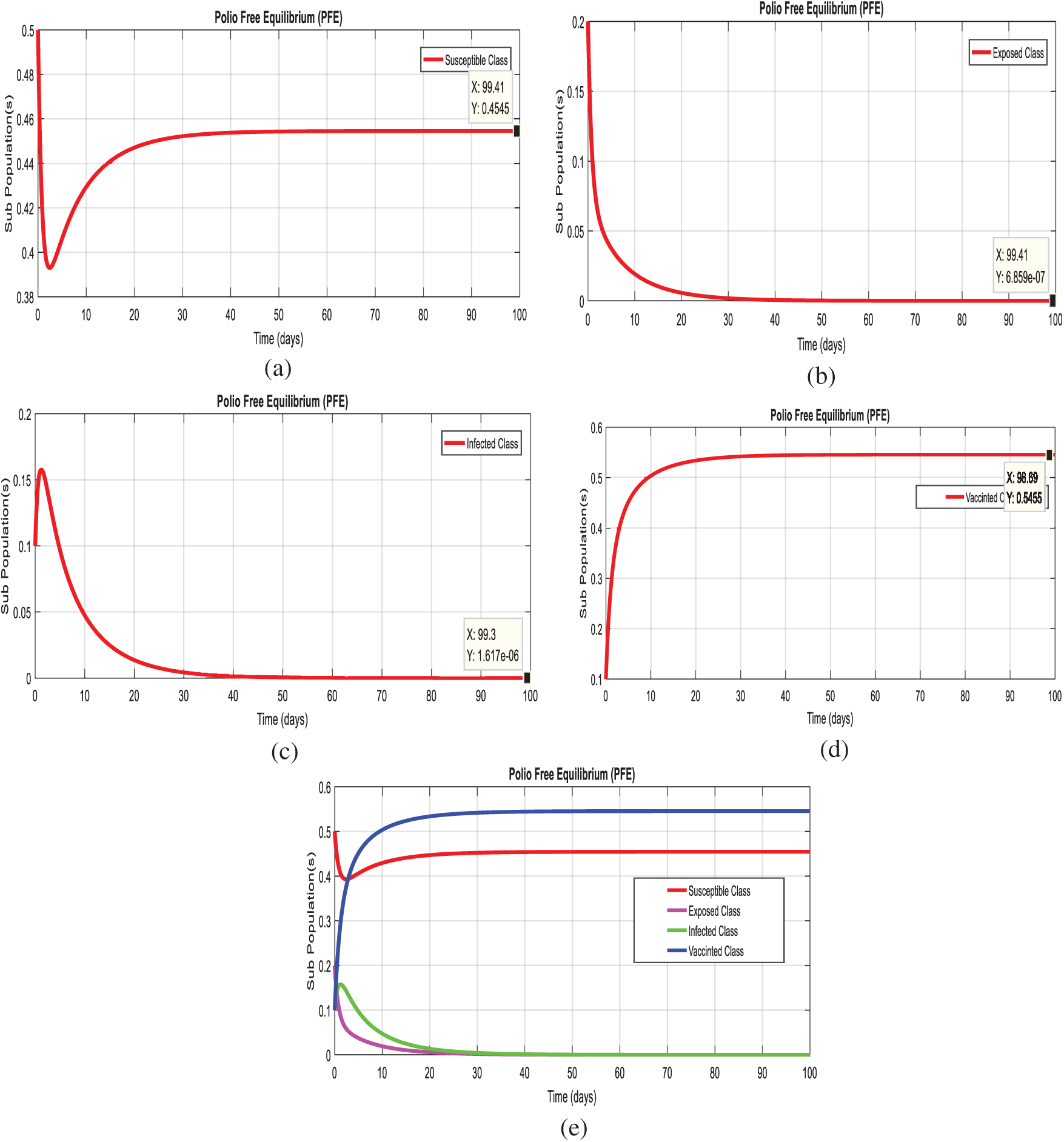
Figure 2: Time plots of the system (1–4) at the polio free equilibrium of model. For any time t (a) Susceptible class (b) Exposed class (c) Infected Class (d) Vaccinated class (e) Combined behavior of each sub-population(s)

Example 2: (Simulation at polio existing equilibrium (PEE−P2) without delay)

Figs. 3a–3d, displays the solution of the system (1–4), at the diarrhea existing equilibrium (PEE−P2), P2=(S∗,E∗,I∗,V∗)=(0.3411,0.0895,0.1604,0.4094), Therefore, the system (1–4) converges to P2, in the absence of delay the value of reproduction number is R0 = 1.4950 > 1. Moreover, Fig. 3e, shows combine behavior of the system (1-4) without consideration of the delay effect, as desired

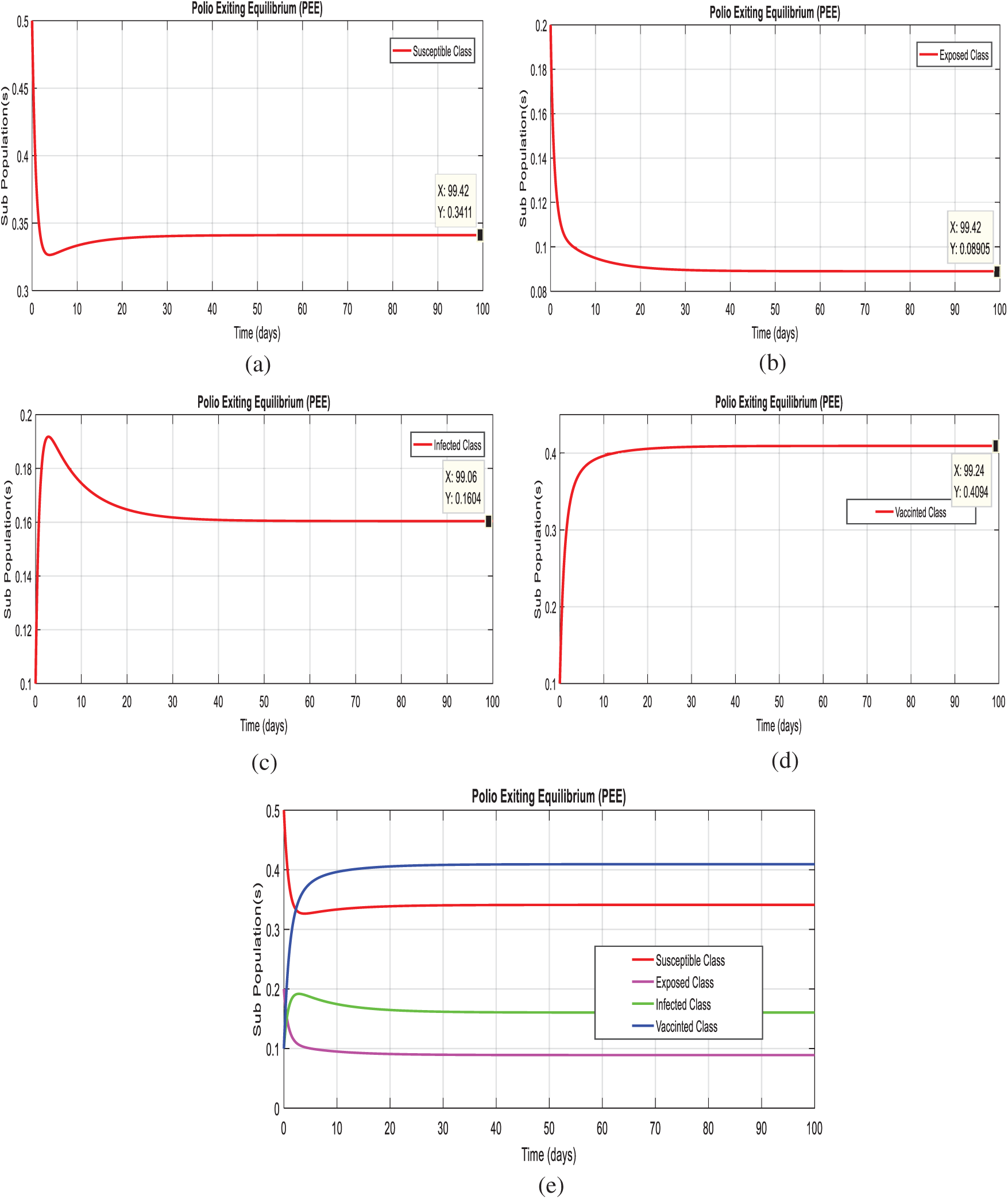
Figure 3: Time plots of the system (1–4) at the Polio existing equilibrium of model. For any time t (a) Susceptible class (b) Exposed class (c) Infected Class (d) Vaccinated class (e) Combined behavior of each sub-population(s)

Example 3: (Simulations at polio existing equilibrium with time delay effect)

In this section, we taken the effect of the system (1–4), at the diarrhea existing equilibrium of the model with effective use of artificial delay tactics. Figs. 4a–4c, we can observe the susceptibility of humans increases with use of delay tactics. In the other hand, we can observe the infectivity of polio patient decreases and even converges to zero.

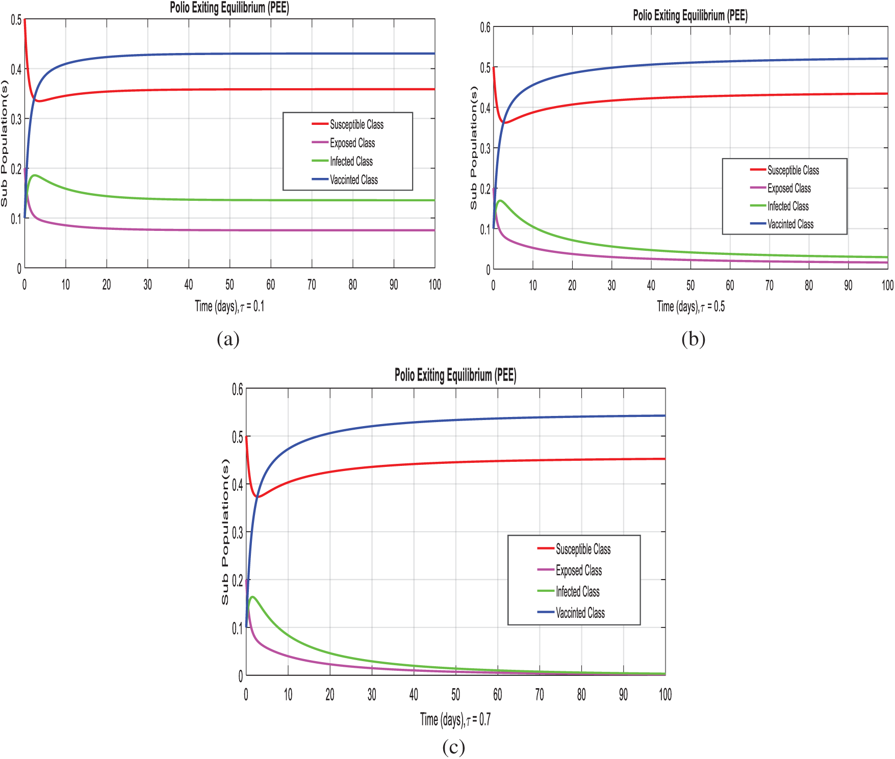
Figure 4: Time plots of the system (1–4) at the polio existing equilibrium with the effective uses of delay tactics. (a) Combined behavior at τ=0.1 (b) Combined behavior at τ=0.5 (c) Combined behavior at τ=0.7

Example 4: (Effectiveness of delay tactics on the reproduction number of the model).

Let, τ=1.011. As clear, the reproduction value decreases that moves the dynamics of the system of polio virus moves from existing scenario to polio free equilibrium. Yet, Fig. 5 displays the fact that the increases in delay strategy can overcome the infectivity of polio viruses, as needed.

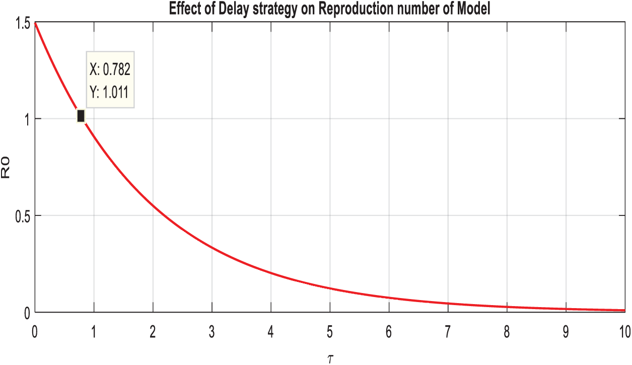
Figure 5: Comparison graph of the reproduction number and artificial delay term of the model

Example 5: (Replication for the consequence of delay term on the infective class).

For the different values of τ, exhibits that infective class of peoples reduces even completely die out from population. Subsequently, Fig. 6 displays the fact that the delay strategies such as vaccinations in different age groups, as desired.

Figure 6: Display of the effect of delay term on infective class of the model

Example 6: (2D-simulations of the system with delay effect).

In this section, we plotted two-dimensional behavior of the model with the effective uses of artificial delay techniques. Even though, theses simulations are the interaction of susceptible class with remaining compartments of the model. Figs. 7a–7c, exhibits that immunity of human’s dominant with the immunity of infected humans, as desired.

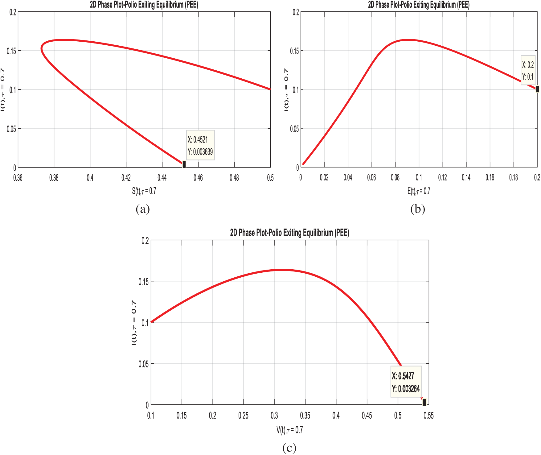
Figure 7: 2-D phases of the system (1–4) with delay effect. (a) Susceptible and infected classes at τ=0.7 (b) Infected and exposed classes at τ=0.7 (c) Vaccinated and infected classes at τ=0.7

6  Conclusion

In this article, we investigated the dynamics of the polio delayed epidemic model with the effective use of delay strategies. In which we divided the entire population into four different groups which are susceptible, exposed, infected and vaccinated. We have calculated the reproduction number for the polio delayed epidemic model and also gave the sensitivity analysis of the parameters involved in reproduction number. We have also presented the local and global stabilities of the model at the equilibrium of the model, that is, at polio-free equilibrium and at polio existing equilibrium by using well-known results of mathematics. In addition, we carefully studied the effect of delay factor on infected class, exposed class and reproduction number and we have come to the conclusion that we can control the dynamics of polio by using different effected techniques of delay like vaccination is proved to be the ultimate solution to avoid the spread of this disease. Immunization is much important and is recommended for children’s who fall under the age group of 2 to 18 months. Moreover, Booster doses are recommended for children’s up to 12 years of age to make sure of immunization. And most importantly a good hygiene system at a personal level is much needed to adapt, which can play a vital role to reduce the spread of the poliovirus.

Funding Statement: The authors received no specific funding for this study.

Conflicts of Interest: The authors declare that they have no conflicts of interest to report regarding the present study.

This work is licensed under a Creative Commons Attribution 4.0 International License, which permits unrestricted use, distribution, and reproduction in any medium, provided the original work is properly cited.