DOI:10.32604/cmc.2022.019705
| Computers, Materials & Continua DOI:10.32604/cmc.2022.019705 | |
| Article |
Data-Driven Self-Learning Controller for Power-Aware Mobile Monitoring IoT Devices
VSB–Technical University of Ostrava, Department of Cybernetics and Biomedical Engineering, Ostrava, 708 00, Czech Republic
*Corresponding Author: Michal Prauzek. Email: michal.prauzek@vsb.cz
Received: 22 April 2021; Accepted: 22 June 2021
Abstract: Nowadays, there is a significant need for maintenance free modern Internet of things (IoT) devices which can monitor an environment. IoT devices such as these are mobile embedded devices which provide data to the internet via Low Power Wide Area Network (LPWAN). LPWAN is a promising communications technology which allows machine to machine (M2M) communication and is suitable for small mobile embedded devices. The paper presents a novel data-driven self-learning (DDSL) controller algorithm which is dedicated to controlling small mobile maintenance-free embedded IoT devices. The DDSL algorithm is based on a modified Q-learning algorithm which allows energy efficient data-driven behavior of mobile embedded IoT devices. The aim of the DDSL algorithm is to dynamically set operation duty cycles according to the estimation of future collected data values, leading to effective operation of power-aware systems. The presented novel solution was tested on a historical data set and compared with a fixed duty cycle reference algorithm. The root mean square error (RMSE) and measurements parameters considered for the DDSL algorithm were compared to a reference algorithm and two independent criteria (the performance score parameter and normalized geometric distance) were used for overall evaluation and comparison. The experiments showed that the novel DDSL method reaches significantly lower RMSE while the number of transmitted data count is less than or equal to the fixed duty cycle algorithm. The overall criteria performance score is 40% higher than the reference algorithm base on static confirmation settings.
Keywords: 5G and beyond wireless; IoT; LPWAN; M2M; Q-learning
The article deals with the design and application of the control algorithm for a prototype of an efficient Low-Cost, Low-Power, Low Complexity—hereinafter (L-CPC) bidirectional communication system for the reading and configuration of embedded devices. Low Power Wide Area Networks (LPWANs) and the fifth-generation technology standard for broadband cellular networks (5G) are promising technologies for the connection of compact monitoring mobile embedded devices to the internet using machine to machine (M2M) communications [1–4]. Monitoring mobile devices are usually deployed as remote data collection systems which can obtain parameters of interest from various application areas (Environmental monitoring, Smart Homes, Smart Cities, Smart Metering, etc.) [5–13]. This area relates to Internet of things (IoT) domain, that allows data transmission from mobile embedded devices to internet clouds [14–15]. In IoT application areas which attempt to attain certain positional estimations of targets, the received signal strength based on the least squares triangulation approach is used [16]. LPWAN standards and 5G technology are suitable for long-term operational devices equipped with low-capacity energy storage, or maintenance-free devices possibly equipped with energy harvesting modules [17–18]. Mobile monitoring devices have many research challenges aimed at ultra-low power consumption demands [19–22]. To address these constraints, there is a significant need for smart software control algorithms using machine learning principles for automated and intelligent device management [23–25].
Generally, reinforcement learning (RL) methods are suitable as easy-to-implement and low computational power demanding machine learning approach for mobile IoT devices [26–29]. RL belongs to the family of semi-supervised learning approaches [30]. It has an agent which takes actions from a possible action set and the environment returns a reward feedback [31]. In this contribution, a Q-learning (QL) method which belongs to the RL-based approaches is implemented. The presented QL Predictive Data-Driven Self-Learning (DDSL) algorithm allows the design of a control procedure based on the duty-cycle data prediction scenario. The major advantage of the presented approach is that the controller and its internal policy are not directly dedicated to a specific application area or the collected data itself; this method uses universal principles to estimate optimal duty-cycle scenario. Therefore, the DDSL algorithm automatically builds domain-based knowledge during on-site operation without any pre-deployment learning procedure.
Several research articles have used various implementations of RL principles, especially QL in monitoring IoT devices at a network level (see Tab. 1). QL algorithms can be used to iteratively change the MAC protocol parameters by a defined policy to achieve to a low energy state [32]. The TDMA-based adaptive task scheduling [33] method or two-tier data dissemination schemes based on Q-learning (TTDD-QL) [34] are energy efficient for wireless sensor networks (WSN). A cooperative energy-efficient model is presented in the article [35], where clustering, mobile sink deployment and variable sensing collaboratively improve the network lifetime. Besides routing-based or cooperative optimization, there are other research challenges which implement the QL procedure in mobile IoT devices or WSN. Future incoming solar energy can be predicted with Q-learning solar energy prediction (QL-SEP) [36], which is useful for solar-powered devices. In [37], an optimal energy management strategy of a portable embedded system based on QL was proposed to extend system lifetime. The QL algorithm also proved to be a suitable solution in terms of energy for wireless embedded systems such as sensor nodes and smartphones [38]. A dynamic energy-efficient system based on the QL technique to control the energy management issue is used in real-time systems in embedded devices [39]. Based on the presented state-of-the-art review (see Tab. 1), the authors stated that several research works describe the use of QL to achieve power effective solutions in embedded systems, although research works exploring data-driven power-aware approaches using QL have not been published yet.
In this article, the application of a novel DDSL control approach for mobile monitoring IoT devices based on wake-up scheduling (Fig. 1) is presented. The core of the algorithm is to dynamically set an operation period through a wake-up timer configuration according to the correct estimation of future collected data values, which potentially leads to effective operation of power-aware systems. For evaluation purposes, there were used historical incoming solar irradiance data from an environmental monitoring device. The presented self-learning algorithm was also evaluated by a set of various QL expert parameter configurations. Predicted values were compared to the collected values from sensors to provide input parameters for the learning process. The testing procedure compares a complete set of collected data and a reduced set with linear interpolation. The article's novelty lies in modification of the QL approach to allow energy efficient data-driven behavior of embedded IoT devices.
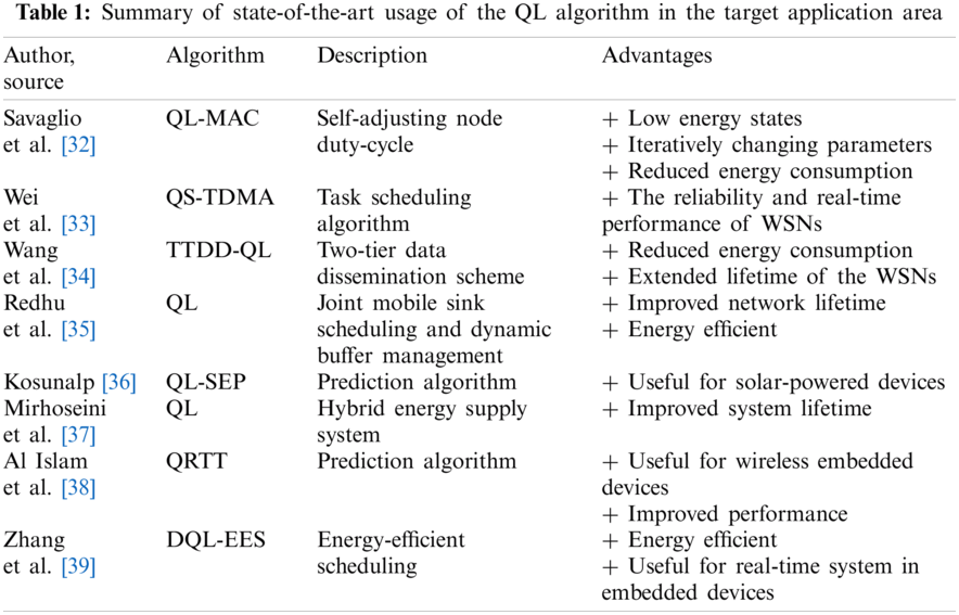

Figure 1: General application principle of a DDSL controller: The mobile device collects and stores parameters of interest into memory. The DDSL controller sets a data collection duty cycle and updates the algorithm through data-driven learning
The remainder of the article is organized as follows: the background section describes power-aware challenges, the general Q-learning algorithm principle and future value estimation by polynomial approximation. The experimental section describes a designed controller, reference algorithm and the evaluation criteria. The experiment summary is elaborated in the results section, followed by a technical discussion. The final section concludes the article and discusses several research challenges as future work.
This section introduces the theoretical background for a general description of the Q-learning algorithm and mathematical formalization of the applied polynomial approximation.
QL belongs to a family of reinforcement learning methods which explore an optimal strategy for a given problem. This semi-supervised model free algorithm was introduced by Watkins [40] and is formulated as a finite Markov decision process, which is a mathematical formalization of the underlying decision-making process.
The QL defines an agent which is responsible for the selection of action
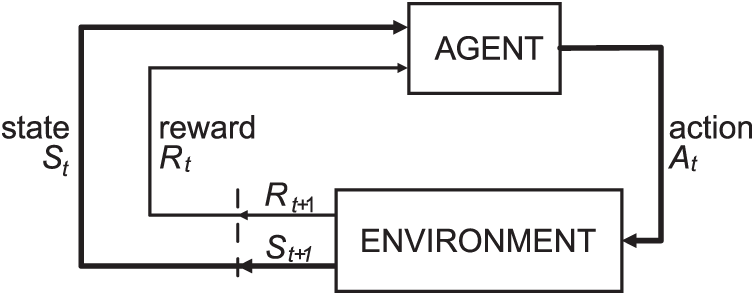
Figure 2: Block diagram of reinforcement learning formalization: The agent plans actions and environment provides feedback (current state and reward)
The QL approach also uses a memory-stored array which is called Q-table, and its size is defined by the number of states S and actions A. The array's columns represent the quantitative values of possible actions. The QL algorithm is controlled by the following equation:
where α is a learning rate which controls the convergence speed of the learning process. When α = 0, the algorithm uses only previous estimates of the reward signal; otherwise α = 1, and the algorithm applies only new knowledge.
The learning strategy is also influenced by a constant ɛ (epsilon-greedy policy), which causes the selection of a random action instead of the maximal reward action. From the 0 to 1 interval, ɛ is selected (e.g., 0.95 means 5% of random actions) [31].
The polynomial approximation interpolates values with a polynomial. The polynomial is a function which is written in the form:
where
An approximation is an inaccurate expression of some function. In this paper, the polynomial coefficients are calculated using the least-squares approximation method by summing squared values of the deviations; this sum should be minimal (see Eq. (3)),
where
The experiment uses the dataset from an environmental data collection station. The data include values of incoming solar energy as simulated input from a sensor. The solar energy values were collected continuously for five years at the Fairview Agricultural Drought Monitoring station (AGDM) located in Alberta, Canada [41], coordinates at 56.0815° latitude, −118.4395° longitude, and 655.00 m elevation. This dataset contains the total incoming solar radiance in W/m2 collected per five-minute interval.
The aim of the performed experiment is evaluation whether the DDSL controller is capable of finding an optimal strategy for dynamic configuration of the data collection period. A conventional QL algorithm was modified to be useful to the proposed experiment for its application in wake-up embedded devices. The experiment was performed in MATLAB, and a complete solution is simple to implement to mobile monitoring devices.
The proposed DDSL controller dynamically sets an operation period according to correct estimation of the collected data to adjust the operation duty cycle. The DDSL controller follows the RL model shown on the Fig. 2. The core of the DDSL controller algorithm is the selection of action A, the subsequent change of environment to state S, and the reward which depends on the selected action and caused state. The self-learning process of the DDSL controller is based on the QL approach.
Action A, which represents a period (time slot)
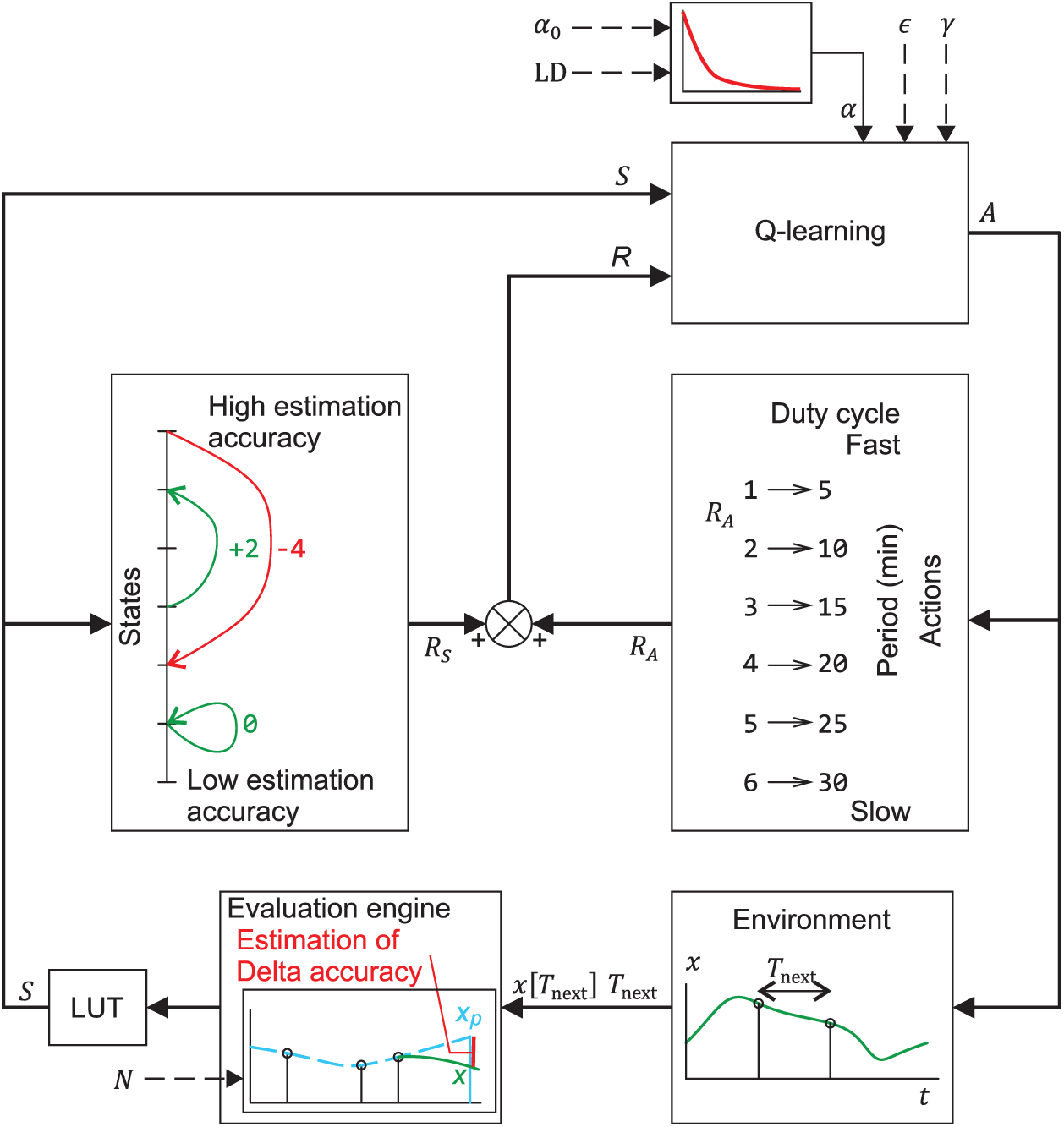
Figure 3: Block diagram of the DDSL controller: The Q-learning block selects action A, which causes the environment feedback (state S and reward R) to control the self-learning process
Based on the current state and performed action, partial rewards (the state reward (
The index_of() function returns an one-based order of elements in the state vector (higher index represents higher estimation accuracy). The
In this case the index of() function provides higher value for longer duty cycle. The total reward R is formulated as sum of
The QL process is affected by a total reward R and current state S with variable configuration of expert constants (α, ɛ, γ). The action A selected by the QL policy is the output of the QL block.
The DDSL approach is equipped by discounting the learning factor to achieve stability in the learning process. The discounting progress of the parameter α is shown in the Fig. 4. In each step of the algorithm, α is discounted by learning discount (LD), especially
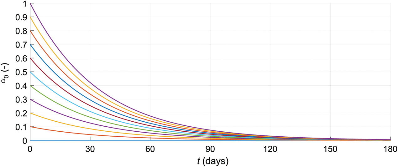
Figure 4: Learning strategy: α discount process for various initial
The conventional QL algorithm presented in the literature [42] is not directly applicable to the proposed experiment. Therefore, there were designed a modification of the original algorithm. The difference between the conventional QL and the modified version is shown in following algorithm descriptions.
The conventional Q-learning algorithm described in [42] is composed of the following commands:
1: Initialize
2: while true do
3: Choose A from S using policy derived from Q (e.g., epsilon-greedy policy)
4: Take action A
5:
6:
7: end while
The modified Q-learning algorithm is composed of the following commands:
1: Initialize
2: while true do
3: Wake up
4: Observe
5: Calculate reward R from
6:
7: Choose A from S using policy derived from Q (e.g., epsilon-greedy policy)
8: Start action A
9: Sleep
10: (time)
11:
12: end while
In the original QL algorithm, the performed action step is inside the QL algorithm loop, but from the monitoring device point of view, the performed action itself is a duration of standby or sleep mode. In the modified scenario, the algorithm performs an action at a different stage than the original approach. The learning process part is completed based on the past state and current state because the future action is unknown.
In the conventional QL algorithm, an action is first selected according to the QL policy and the environment state. The action is performed, and a reward based on the previous state and actual action is calculated. In the next step, the Q-table is updated by the learning process and a new state S is observed. However, in the modified QL, the loop also starts by selecting and performing an action, but then implements a new variable called sleep. This variable represents the action, the selected sleep time. Then the reward from the previous state and action is calculated and the Q-table is updated by the learning process itself.
The modified QL algorithm is controlled by the following equation:
where α is a learning rate.
The polynomial approximation method is used to evaluate the next value
In the next step, MATLAB's polyval function is used to protect negative values in prediction. The polyval evaluated the polynomial p at each point x (see Eq. (2)). The p is a vector of the coefficients and the point x is the index value of the action in the specific simulation step. If the final polyfit evaluation value is greater than or equal to 0, the polyval function result is the
3.2 Reference Solution and Evaluation Criteria
To evaluate the DDSL controller approach, a reference algorithm with a linear interpolation method is used. The original collected data has a 5-min data collection interval. Therefore, the reference solution is based on an original data set where only 10-, 15-, 20-, 25- and 30-min intervals are extracted. To fill in the missing data between the extracted samples, the linear interpolation method was used.
To compare the accuracy of prediction between individual settings of expert constants and the reference solution, the root mean squared error (RMSE) was calculated by following equation,
where n is the size of the data set,
The Number of Measurement (NoM) is the second evaluation parameter which follows the number of the operation period. The algorithm policy is principally designed to minimize NoM (
The performance score (PS) is then the overall evaluation parameter, which considers both above-mentioned parameters (RMSE and the NoM) and is calculated according to the following equation:
where
Generally, an overall evaluation considers two parameters (RMSE and NoM). Technically, these parameters oppose each other, and a trade-off between RMSE and NoM should be considered. To evaluate the DDSL approach, a cartesian distance to zero is used.
The RMSE and NoM parameters are normalized according to the worst case, meaning a 30-min reference algorithm RMSE parameter and a 5-min reference algorithm NoM parameter:
An overall cartesian evaluation parameter
This section provides the results of a comprehensive set of experiments which verify the designed controller with various QL parameters settings and the degree of the polynomial. Each experiment configuration was repeated ten times to eliminate the effect of the epsilon-greedy policy. Experiments were performed with the following settings for
•
• γ = {0, 0.1, 0.2, …, 1},
• N = {1, 2, 3, 4, 5}.
Fig. 5 shows an overall comparison of the reference algorithm and the DDSL controller and the highest PS results for various degrees of the polynomial for the DDSL controller. The DDSL controller provides approximately 40% higher PS than the best reference algorithm, with the exception of the degree of polynomial N = 5, which provides only 23% higher PS. The Tab. 2 provides a numerical summary of the highest PS algorithm settings. The highest PS results provided the algorithm with low
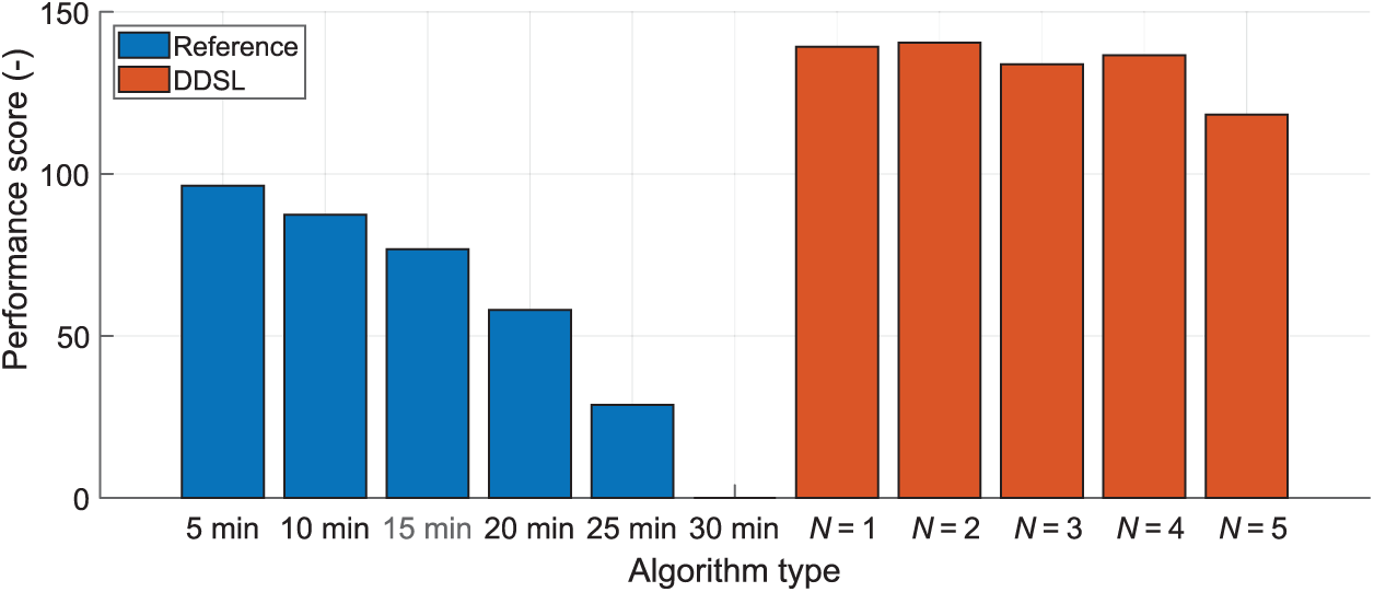
Figure 5: Overall comparison of the reference algorithm and DDSL controller for the degree of the polynomial
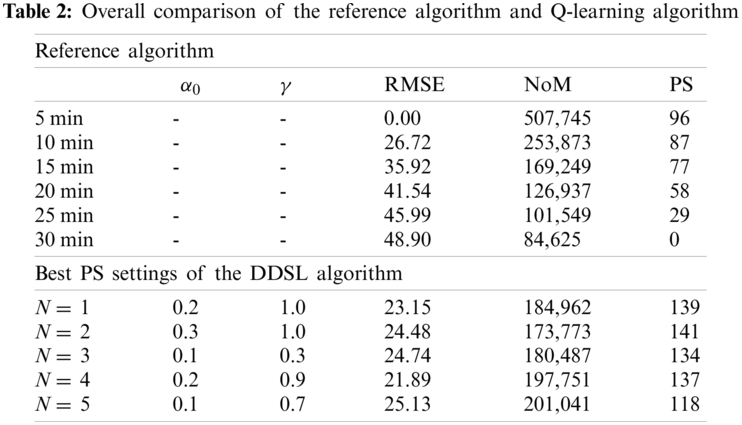
Fig. 6 provides a distribution of the algorithm PS with various
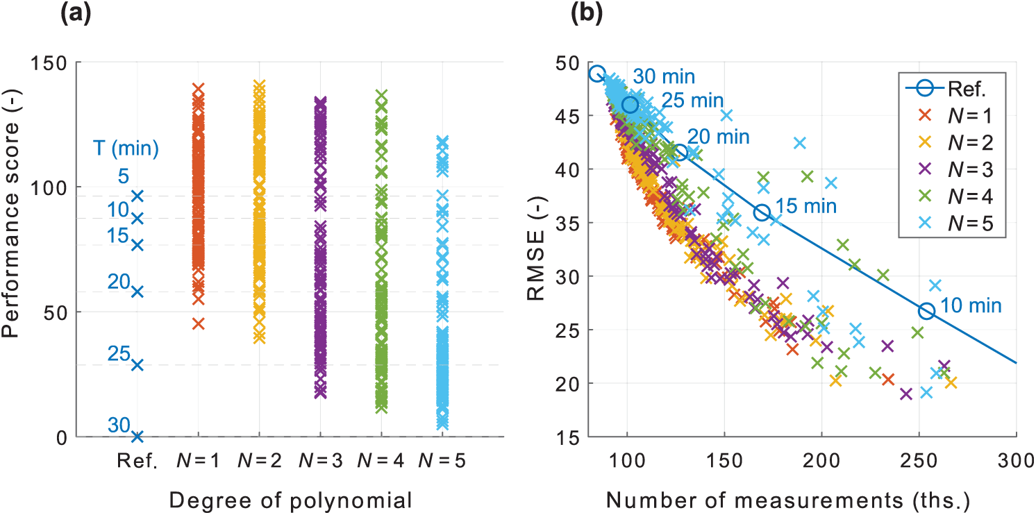
Figure 6: Comparison with the reference algorithm. (a) Performance for various settings of
Fig. 6b shows the DDSL controller result in cartesian coordinates. The x-axis represents the NoM and the y-axis describes the RMSE. This representation provides a reference algorithm borderline which divides the two-dimensional cartesian coordinate system into two parts. The first part above the reference algorithm borderline means, that the algorithm achieves worse PS than the reference approach. The results beneath the reference algorithm borderline return at least a lower RMSE with the same NoM as the reference algorithm or lower NoM with the same RMSE as the reference algorithm, respectively. A geometric distance to zero is a crucial evaluation parameter. The weights of the x- and y-axis should be considered or normalized to balance the effect of the RMSE and NoM parameters (parameter
Fig. 7 shows 3D bar graphs for various α and γ for the degree of polynomial 1 and 2. There can be observed an increase of PS for
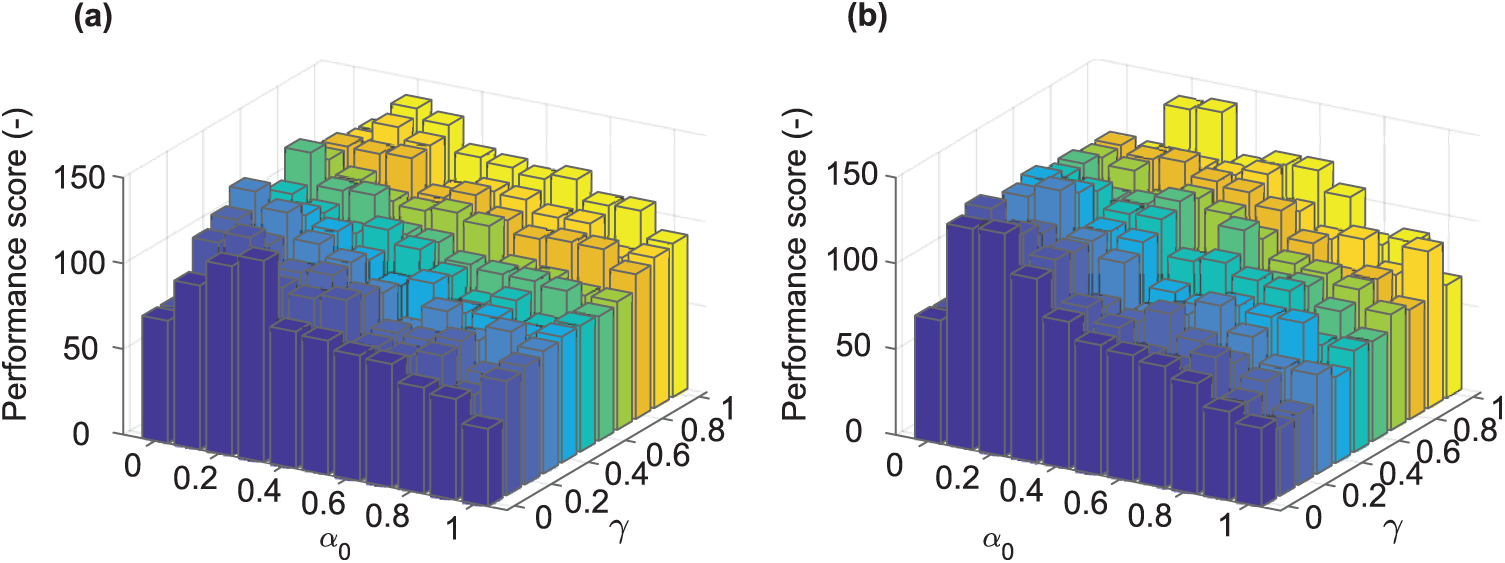
Figure 7: PS of the Q-learning algorithm with various settings of
Fig. 8 shows a subset of the bar graphs for various degrees of polynomial for

Figure 8: PS of the Q-learning algorithm with selected learning rate
Fig. 9 represents the PS in a cartesian coordination system for the degree of the polynomial
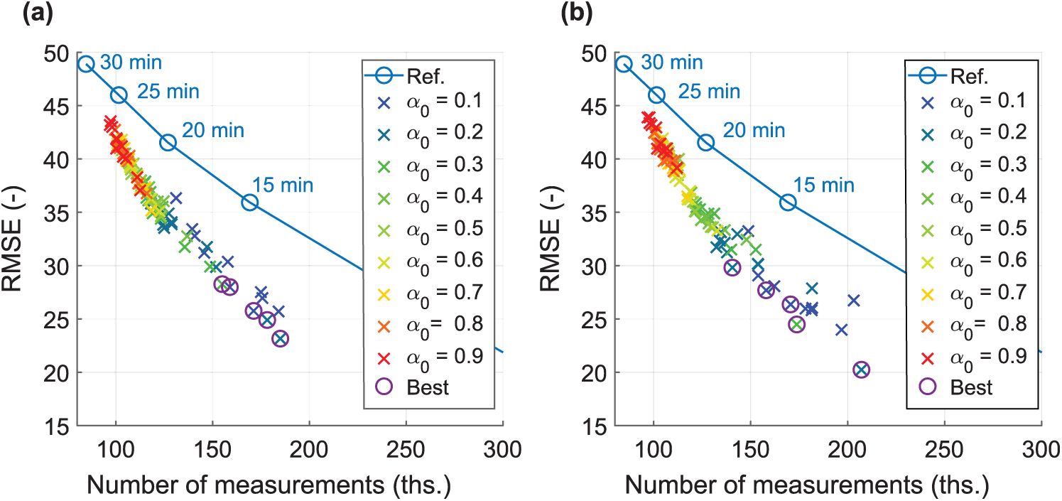
Figure 9: Location of various settings of α and γ in cartesian coordinates. (a)
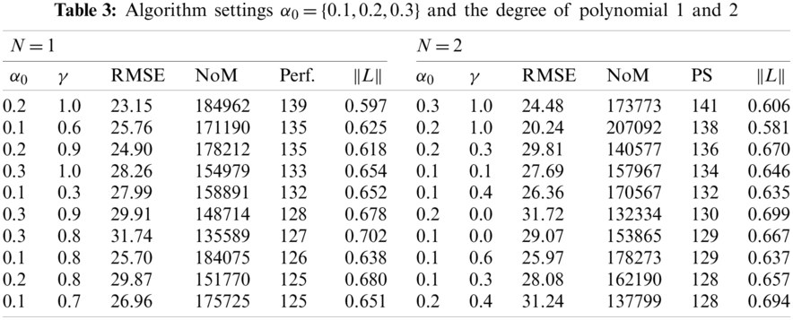
Tab. 3 provides a numerical summary of the performed experiments. It shows only the ten best cases. The best algorithm reached PS 141 with
The results return several interesting areas to discuss. The first idea concerns the correct selection of the degree of polynomial. The presented experiment used a degree of polynomial from 1 to 5. Based on the input solar irradiance data, the DDSL approach provided the best performing result for the degree of the polynomial 2. The degree of the polynomial 1 also provided better performance than 3, 4 and 5 in this case. It must be highlighted that selection of the appropriate degree of the polynomial is directly linked to the type of data collected from the sensors. In our case, the best performing result was achieved by linear or quadratic approximation represented by the degree of the polynomial 1 and 2. In the case of a different dataset, correct selection of the coefficient could lead to higher degree of the polynomial. Regarding the key feature of the DDSL approach, exploratory studies for suitable degrees of the polynomial should be performed before mobile monitoring IoT devices are deployed in target application areas. The capability of the self-learning approach is limited without custom adjustment of the degree of the polynomial according to the character of the collected data.
The configuration of Q-learning parameters is second area to discuss. Deployment of the mobile monitoring devices should consider proper selection of the learning rate, discount factor, and the epsilon-greedy policy. The article's results showed that the initial learning rate should be set conservatively from 0.1 to 0.3. Therefore, the DDSL controller accepts new information slowly and keeps its already obtained knowledge stored in a Q-table. However, in terms of the discount factor, there is no conclusive result. With a degree of polynomial 1, the experiment showed that the best results are achieved from high cumulative discount factor approaches (0.8–1). However, the result which included a degree of polynomial 2 showed that an instant reward policy with a low discount factor (<0.4) could also lead to the best performance solutions. Therefore, the discount factor setting is not simply a subject of the input dataset but has a strong connection to the degree of the polynomial. The epsilon-greedy policy is set to 5% of random actions as standard in such applications, but the question is whether this leads to the best performance in long-term deployments where the learning rate is significantly reduced by the learning discount coefficient. This idea should be evaluated with long-term field testing or extensive simulations on an extended dataset. In this case however, the study does not provide a general answer for setting up the initial epsilon-greedy and discount policies.
The final discussion topic concerns the evaluation policy of the presented solution. There were designed two basic approaches, one which uses a linear ratio between the RMSE and NoM, and the second which is calculated by the geometrical distance in normalized cartesian space. Both evaluation methodologies followed the same aim, which was to determine an evaluation coefficient which targets the tradeoff between low RMSE and low NoM. Both methodologies provide similar results in an opposing manner, one maximizing the linear ratio and the other minimizing the normalized distance. In another implementation scenario, the evaluation strategy varied according to the specific optimization target.
Tab. 4 shows a general comparison of the DDSL controller approach with three QL state-of-the-art methods. The stated studies [43–45] used data-driven QL approaches to solve their control requirement in addition to the DDSL controller. The major difference between the individual approaches is the way the QL algorithm is used, the possible additional methods for control, and the monitored subject matter. The advantages and limitations mentioned in the table are derived from these conditions. The proposed DDSL controller offers a unique approach in solving a data-driven self-learning principle for mobile monitoring embedded devices.

The article proposed a modified QL-based algorithm which controls an operational cycle according to the acquired data. The general principle lies in observation of the parameters of interest when data from sensors contains high information value. This solution leads to the minimization of operational cycles when data changes according to a predictable trend. This solution offers a unique paradigm in contrast to the classic scenario of an embedded device obtaining data and then deciding whether the data contains information which should be stored and transmitted to a cloud. The presented DDSL method principally avoids redundant data acquisition, which leads to a more energy-efficient operation.
The proposed DDSL algorithm provides better results than the reference algorithm which operates with a continuous measurement period. The novel approach described in this paper achieved an approximately 40% higher PS than the reference algorithm. It means that our novel algorithm reached a lower RMSE at the same NoM as the reference algorithm, or a lower NoM at the same RMSE.
The presented solution opens several research opportunities. The first challenge includes application of the proposed method in another data domain. The next research challenge might be modification of the learning model. It is also possible to use statistical parameters as a reward policy to replace the polynomial function. In this article, the authors examined the general principle of the DDSL approach, which performs well on the presented mobile monitoring embedded devices, however future modification of the DDSL approach could lead to more effective domain-customized solutions.
Funding Statement: This work was supported by the project SP2021/29, “Development of algorithms and systems for control, measurement and safety applications VII” of the Student Grant System, VSB-TU Ostrava. This work was also supported by the European Regional Development Fund in the Research Centre of Advanced Mechatronic Systems project, Project Number CZ.02.1.01/0.0/0.0/16_019/0000867 under the Operational Programme for Research, Development and Education. This work has received funding from the European Union's Horizon 2020 research and innovation programme under grant agreement N°856670.
Conflicts of Interest: The authors declare that they have no conflicts of interest to report regarding the present study.
1. B. S. Chaudhari, M. Zennaro and S. Borkar, “LPWAN technologies: Emerging application characteristics, requirements, and design considerations,” Future Internet, vol. 12, no. 3, Article no. 46, 2020. [Google Scholar]
2. Q. Zhao, “Presents the technology, protocols, and new innovations in industrial internet of things (IIoT),” Internet of Things for Industry 4.0, pp. 39–56, 2020. [Google Scholar]
3. T. Ramathulasi and M. R. Babu, “Comprehensive survey of IoT communication technologies,” Emerging Research in Data Engineering Systems and Computer Communications, pp. 303–311, 2020. [Google Scholar]
4. W. Ayoub, F. Nouvel, A. E. Samhat, M. Mroue and J. C. Prevotet, “Mobility management with session continuity during handover in LPWAN,” IEEE Internet of Things Journal, vol. 7, no. 8, pp. 6686–6703, 2020. [Google Scholar]
5. G. Pathak, J. Gutierrez and S. U. Rehman, “Security in low powered wide area networks: Opportunities for software defined network-supported solutions,” Electronics, vol. 9, no. 8, Article no. 1195, 2020. [Google Scholar]
6. J. A. Onumanyi, A. M. Abu-Mahfouz and G. P. Hancke, “Low power wide area network, cognitive radio and the internet of things: Potentials for integration,” Sensors, vol. 20, no. 23, Article no. 6837, 2020. [Google Scholar]
7. G. B. Gaggero, M. Marchese, A. Moheddine and F. Patrone, “A possible smart metering system evolution for rural and remote areas employing unmanned aerial vehicles and internet of things in smart grids,” Sensors, vol. 21, no. 5, Article no. 1627, 2021. [Google Scholar]
8. E. Saavedra, G. Del Campo and A. Santamaria, “Smart metering for challenging scenarios: A low-cost, self-powered and non-intrusive IoT device,” Sensors, vol. 20, no. 24, Article no. 7133, 2020. [Google Scholar]
9. K. Seyhan, T. N. Nguyen, S. Akleylek, K. Cengiz and S. H. Islam, “Bi-gISIS KE: Modified key exchange protocol with reusable keys for IoT security,” Journal of Information Security and Applications, vol. 58, Article no. 102788, 2021. [Google Scholar]
10. J. P. Jeong, S. Yeon, T. Kim, H. Lee, S. M. Kim et al., “SALA: Smartphone-assisted localization algorithm for positioning indoor IoT devices,” Wireless Networks, vol. 24, no. 1, pp. 27–47, 2018. [Google Scholar]
11. P. Chanak, I. Banerjee and R. S. Sherratt, “Simultaneous mobile sink allocation in home environments with applications in mobile consumer robotics,” IEEE Transactions on Consumer Electronics, vol. 61, no. 2, pp. 181–188, 2015. [Google Scholar]
12. B. D. Minor, J. R. Doppa and D. J. Cook, “Learning activity predictors from sensor data: Algorithms, evaluation, and applications,” IEEE Transactions on Knowledge and Data Engineering, vol. 29, no. 12, pp. 2744–2757, 2017. [Google Scholar]
13. R. Giuliano, F. Mazzenga and A. Vizzarri, “Satellite-based capillary 5 g-mmtc networks for environmental applications,” IEEE Aerospace and Electronic Systems Magazine, vol. 34, no. 10, pp. 40–48, 2019. [Google Scholar]
14. A. Pekar, J. Mocnej, W. K. Seah and I. Zolotova, “Application domain-based overview of IoT network traffic characteristics,” ACM Computing Surveys (CSUR), vol. 53, no. 4, pp. 1–33, 2020. [Google Scholar]
15. T. Lojka, M. Miškuf and I. Zolotová, “Industrial iot gateway with machine learning for smart manufacturing,” in Ifip Int. Conf. on Advances in Production Management Systems, pp. 759–766, Iguassu Falls, Brazil, Springer, 2016. [Google Scholar]
16. K. Cengiz, “Comprehensive analysis on least squares lateration for indoor positioning systems,” IEEE Internet of Things Journal, vol. 8,pp. 2842–2856, 2020. [Google Scholar]
17. R. Karim, A. Iftikhar, B. Ijaz and I. B. Mabrouk, “The potentials, challenges, and future directions of on-chip-antennas for emerging wireless applications—a comprehensive survey,” IEEE Access, vol. 7, pp. 173897–173934, 2019. [Google Scholar]
18. M. Pointl and D. Fuchs-Hanusch, “Assessing the potential of LPWAN communication technologies for near real-time leak detection in water distribution systems,” Sensors, vol. 21, no. 1, Article no. 293, 2021. [Google Scholar]
19. J. Yan, Z. Kuang, F. Yang and X. Deng, “Mode selection and resource allocation algorithm in energy harvesting D2D heterogeneous network,” IEEE Access, vol. 7, pp. 179929–179941, 2019. [Google Scholar]
20. N. Y. Philip, J. J. Rodrigues, H. Wang, S. J. Fong and J. Chen, “Internet of things for in-home health monitoring systems: Current advances, challenges and future directions,” IEEE Journal on Selected Areas in Communications, vol. 39, no. 2, pp. 300–310, 2021. [Google Scholar]
21. P. K. Sahoo, “Efficient security mechanisms for mHealth applications using wireless body sensor networks,” Sensors, vol. 12, no. 9, pp. 12606–12633, 2012. [Google Scholar]
22. S. Marinkovic and E. Popovici, “Ultra-low power signal-oriented approach for wireless health monitoring,” Sensors, vol. 12, no. 6, pp. 7917–7937, 2012. [Google Scholar]
23. M. Elsisi, K. Mahmoud, M. Lehtonen and M. M. Darwish, “Reliable industry 4.0 based on machine learning and IoT for analyzing, monitoring, and securing smart meters,” Sensors, vol. 21, no. 2, Article no. 487, 2021. [Google Scholar]
24. R. Huang, X. Chu, J. Zhang, Y. H. Hu and H. Yan, “A machine-learning-enabled context-driven control mechanism for software-defined smart home networks,” Sensors and Materials, vol. 31, no. 6, pp. 2103–2129, 2019. [Google Scholar]
25. L. Yin, Q. Gao, L. Zhao, B. Zhang, T. Wang et al., “A review of machine learning for new generation smart dispatch in power systems,” in Engineering Applications of Artificial Intelligence, vol. 88, 2020. [Google Scholar]
26. J. Jagannath, N. Polosky, A. Jagannath, F. Restuccia and T. Melodia, “Machine learning for wireless communications in the internet of things: A comprehensive survey,” Ad Hoc Networks, vol. 93, Article no. 101913, 2019. [Google Scholar]
27. S. Yu, X. Chen, Z. Zhou, X. Gong and D. Wu, “Intelligent multi-timescale resource management for multi-access edge computing in 5G ultra dense network,” IEEE Internet of Things Journal, vol. 8, pp. 2238–2251, 2020. [Google Scholar]
28. I. A. Ridhawi, M. Aloqaily, A. Boukerche and Y. Jararweh, “Enabling intelligent IoCV services at the edge for 5G networks and beyond,” IEEE Transactions on Intelligent Transportation Systems, Early Access, 2021. [Google Scholar]
29. J. Frnda, M. Durica, M. Savrasovs, P. Fournier-Viger and J. C. W. Lin, “Qos to QoE mapping function for IPTV quality assessment based on kohonen Map: A pilot study,” Transport and Telecommunication Journal, vol. 21, no. 3, pp. 181–190, 2020. [Google Scholar]
30. R. S. Sutton and A. G. Barto, Reinforcement Learning: An Introduction, Cambridge, Massachusetts and London, England: The MIT Press, 1998. [Google Scholar]
31. C. J. C. H. Watkins and P. Dayan, “Technical note: Qlearning,” Machine Learning, vol. 8, no. 3, pp. 279–292, 1992. [Google Scholar]
32. C. Savaglio, P. Pace, G. Aloi, A. Liotta and G. Fortino, “Lightweight reinforcement learning for energy efficient communications in wireless sensor networks,” IEEE Access, vol. 7, pp. 29355–29364, 2019. [Google Scholar]
33. Z. Wei, X. Xu, L. Feng and B. Ding, “Task scheduling algorithm based on Q-learning and programming for sensor nodes,” Pattern Recognition and Artificial Intelligence, vol. 29, pp. 1028–1036, 2016. [Google Scholar]
34. N. C. Wang and W. J. Hsu, “Energy efficient two-tier data dissemination based on Q-learning for wireless sensor networks,” IEEE Access, vol. 8, pp. 74129–74136, 2020. [Google Scholar]
35. S. Redhu and R. M. Hegde, “Cooperative network model for joint mobile sink scheduling and dynamic buffer management using Q-learning,” IEEE Transactions on Network and Service Management, vol. 17, no. 3, pp. 1853–1864, 2020. [Google Scholar]
36. S. Kosunalp, “A new energy prediction algorithm for energy-harvesting wireless sensor networks with Q-learning,” IEEE Access, vol. 4, pp. 5755–5763, 2016. [Google Scholar]
37. A. Mirhoseini and F. Koushanfar, “Learning to manage combined energy supply systems,” in IEEE/ACM Int. Symp. on Low Power Electronics and Design, Fukuoka, Japan, pp. 229–234, 2011. [Google Scholar]
38. A. A. Al Islam and V. Raghunathan, “QRTT: Stateful round trip time estimation for wireless embedded systems using Q-learning,” IEEE Embedded Systems Letters, vol. 4, no. 4, pp. 102–105, 2012. [Google Scholar]
39. Q. Zhang, M. Lin, L. T. Yang, Z. Chen and P. Li, “Energy-efficient scheduling for real-time systems based on deep Q-learning model,” IEEE Transactions on Sustainable Computing, vol. 4, no. 1, pp. 132–141, 2017. [Google Scholar]
40. C. J. C. H. Watkins, “Learning from delayed rewards,” Ph.D. dissertation, Cambridge University, 1989. [Google Scholar]
41. “ACIS data products and tools: Alberta agriculture and rural development,” 2013. [Google Scholar]
42. R. S. Sutton and A. G. Barto, Reinforcement Learning: An Introduction. Cambridge, Massachusetts and London, England: The MIT Press, 2018. [Google Scholar]
43. C. Lork, W. T. Li, Y. Qin, Y. Zhou, C. Yuen et al., “An uncertainty-aware deep reinforcement learning framework for residential air conditioning energy management,” Applied Energy, vol. 276, Article no. 115426, 2020. [Google Scholar]
44. M. B. Radac, R. E. Precup and R. C. Roman, “Data-driven virtual reference feedback tuning and reinforcement Q-learning for model-free position control of an aerodynamic system,” in 24th Mediterranean Conf. on Control and Automation, Athens, Greece, pp. 1126–1132, 2016. [Google Scholar]
45. J. Duan, D. Shi, R. Diao, H. Li, Z. Wang et al., “Deep-reinforcement-learning-based autonomous voltage control for power grid operations,” IEEE Transactions on Power Systems, vol. 35, no. 1, pp. 814–817, 2019. [Google Scholar]
 | This work is licensed under a Creative Commons Attribution 4.0 International License, which permits unrestricted use, distribution, and reproduction in any medium, provided the original work is properly cited. |