Computers, Materials & Continua DOI:10.32604/cmc.2022.019695
Article

Bayesian Group Chain Sampling Plan for Poisson Distribution with Gamma Prior

Waqar Hafeez1, Nazrina Aziz1,2,*, Zakiyah Zain1,2 and Nur Azulia Kamarudin1

1School of Quantitative Sciences, Universiti Utara Malaysia, UUM Sintok, 06010, Kedah, Malaysia
2Institute of Strategic Industrial Decision Modelling (ISIDM), Universiti Utara Malaysia, UUM Sintok, 06010, Kedah, Malaysia
*Corresponding Author: Nazrina Aziz. Email: nazrina@uum.edu.my
Received: 22 April 2021; Accepted: 07 June 2021

Abstract: Acceptance sampling is a statistical quality control technique that consists of procedures for sentencing one or more incoming lots of finished products. Acceptance or rejection is based on the inspection of sampled products drawn randomly from the lot. The theory of previous acceptance sampling was built upon the assumption that the process from which the lots are produced is stable and the process fraction nonconforming is a constant. Process variability is inevitable due to random fluctuations, which may inadvertently lead to quality variation. As an alternative to traditional sampling plans, Bayesian approach can be used by considering prior information of the process. Using different combinations of design parameters, this study introduces a Bayesian group chain sampling plan (BGChSP). For the first time in group chain sampling plan, the probability of lot acceptance is derived by using Poisson distribution to estimate an average number of defectives. Gamma distribution is used as a prior distribution with Poisson distribution. Taking into account both consumer’s and producer’s risks, this research considers two quality regions namely, probabilistic quality region (PQR) and indifference quality region (IQR). By minimizing consumer’s and producer’s risks, BGChSP can be used to minimize the average number of defective products in industry.

Keywords: Bayesian; acceptance sampling; gamma; produce risk; consumer risk

1  Introduction

There is tough competition in the industry by rapidly increasing the needs of statistical and analytical techniques towards the improvement of product quality [1–3]. This study is related to Bayesian group chain sampling plan (BGChSP) by using a novel approach called quality region. Instead of considering a point estimate of the quality of a process, this plan is based on a range of quality levels. The producer’s risk and consumer’s risk are associated with every sampling plan [4]. A good plan delivers decision rules of acceptance for both producer and consumer to meet the present quality condition of the product [5]. Improvement in technology is rapidly increasing with the passage of time and supplier needs high-quality products with low defective fraction [6]. Unfortunately, in some situations, traditional methods cannot detect the defective product with such quality level. Thus, quality regions were introduced to overcome such problems [7,8]. By involving probabilistic quality region (PQR) and indifference quality region (IQR), this study designs the parameters for the plan indexed with quality region.

Bayesian approach is based on the combination of current and prior information for the selection of distribution. In acceptance sampling plan, Bayesian approach is required to specify a distribution of defectives from lot to lot [7]. Prior distribution is the expected distribution of the lot quality, that is under inspection. Prior distribution is formulated before taking the sample and empirical knowledge is based on the sample under study called the distribution of sample or data. The combination of prior and empirical information leads to a decision about the current lot either it will be accepted or rejected.

2  Literature Review

Epstein [9] was the first who introduced the idea of single sampling plan (SSP), to distinguish between good and bad lot for zero and one acceptance number. Dodge [10] introduced the chain sampling plan to overcome the deficiency of SSP, with more than one acceptance number and for the general family of chain sampling inspection plan [11]. Under an assumption that cost is linear in p that is the fraction of defectives. Hald [12] provides a system of attribute single sampling plan obtained by minimizing average cost. Later, single sampling plan was modified by using acceptable quality level (AQL) and limiting quality level (LQL) for Bayesian single sampling plan with weighted Poisson distribution [13] and Poisson distribution [14]. Later, in the construction and performance measure, a Bayesian chain sampling plan was discussed for gamma prior [15]. For Beta prior, a Bayesian double sampling plan was considered for the construction and performance measure through quality region [16]. Mathew et al. [17] also work in two-sided complete Bayesian chain sampling plan with Poisson and gamma as prior distribution.

Aslam et al. [18] developed a group sampling plan (GSP), by considering multiple testers at the same time. In GSP the sample size is divided into g number of groups based on the available number of testers n=r∗g. Aslam et al. [19] designed group acceptance sampling plan (GASP) for truncated life tests, with the product lifetime following Pareto distribution of the second kind. Later, for a family of Pareto distribution, an efficient GASP was introduced by Mughal et al. [20]; they assumed the total number of defectives as groups. The number of defectives in the proposed plan was recorded based on all groups instead of an individual group. Moreover, for a family of Pareto distribution, an economic reliability acceptance sampling plan was proposed for an efficient group sampling technique [21]. By satisfying design parameters for a given group and acceptance number, a minimum termination time was required for the proposed plan. Using GASP for Pareto distribution of 2nd kind, an economic reliability group acceptance sampling plan was developed by Mughal et al. [22]. For the biased data theory to find the required design parameters, they used Poisson and weighted Poisson distributions. It was proven that their proposed plans required minimum testing time.

Mughal et al. [23] developed a GChSP plan for the lifetime of a product following Pareto distribution of 2nd kind. Satisfying pre-assumed design parameters at several quality levels, probability of lot acceptance was obtained. Based on their sampling plan, Mughal [24] extended and proposed a generalized GChSP. By considering several values of the proportion of defectives, the minimum sample size and probability of lot acceptance were found to satisfy pre-specified consumer's risk. Recently, Hafeez et al. [25] also worked on this plan and estimated AQL and LQL for the average proportion of defective products in their study.

Based on Mughal et al. [23] plan, this study concerns with the development of a Bayesian group chain sampling plan (BGChSP). In group chain sampling plan, the probability of lot acceptance is derived by using Poisson distribution and gamma is used as a prior distribution. For PQR and IQR, this study designs the plan indexed parameters which are: AQL, LQL, producer’s risk α, consumer’s risk β, for the specified values of the number of testers r and shape parameter s. Also, the numerical illustrations are provided for prior distribution parameters.

3  Methodology

The operating procedure for the proposed plan is based on the following steps:

1.    Select an ideal number of g groups for each lot and assign r items to each group with the sample size required n=g∗r.

2.    Count the number of defectives d.

3.    If d=0, accept the lot.

4.    If d>1, reject the lot.

5.    If d=1, and no defectives was found in the immediately preceding i samples, then accept the lot.

All the above steps can be summarized in a flow chart presented in Fig. 1.

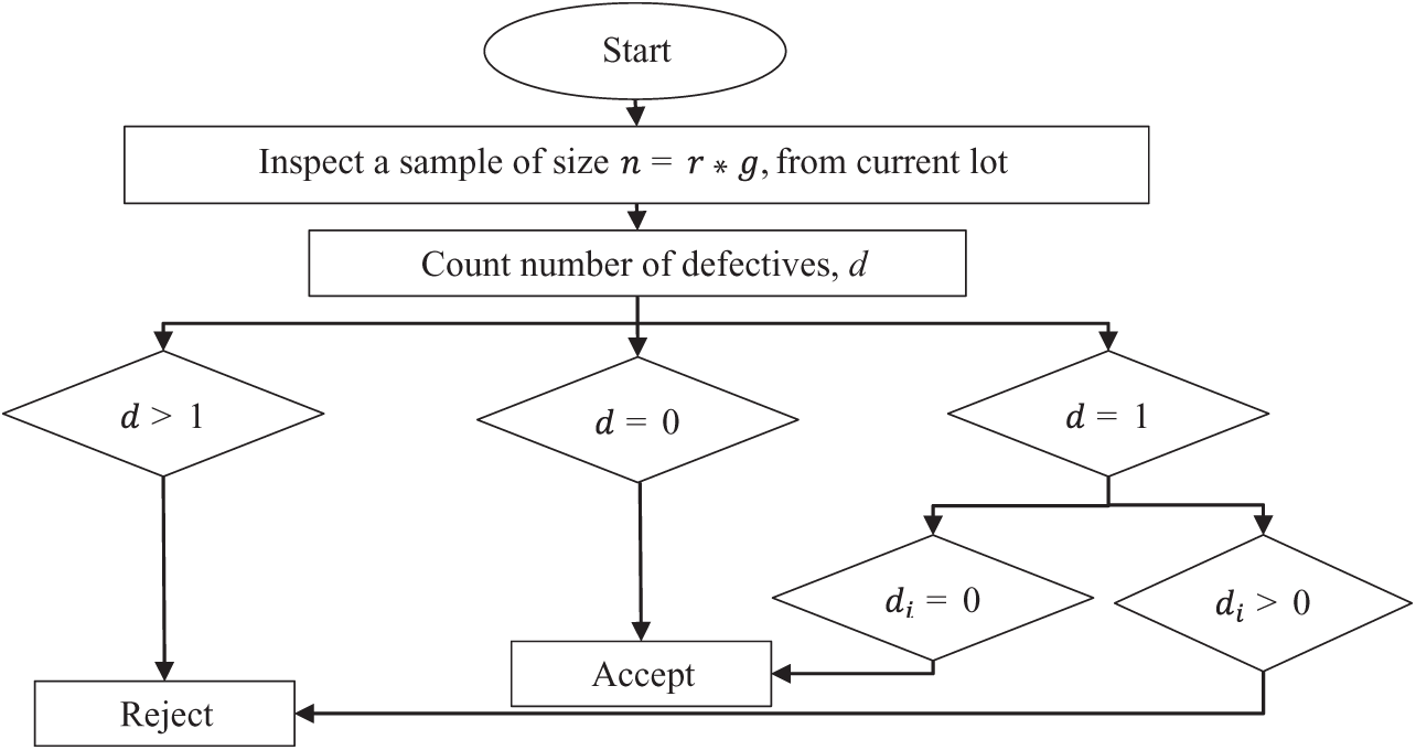
Figure 1: Operating procedure of the proposed sampling plan

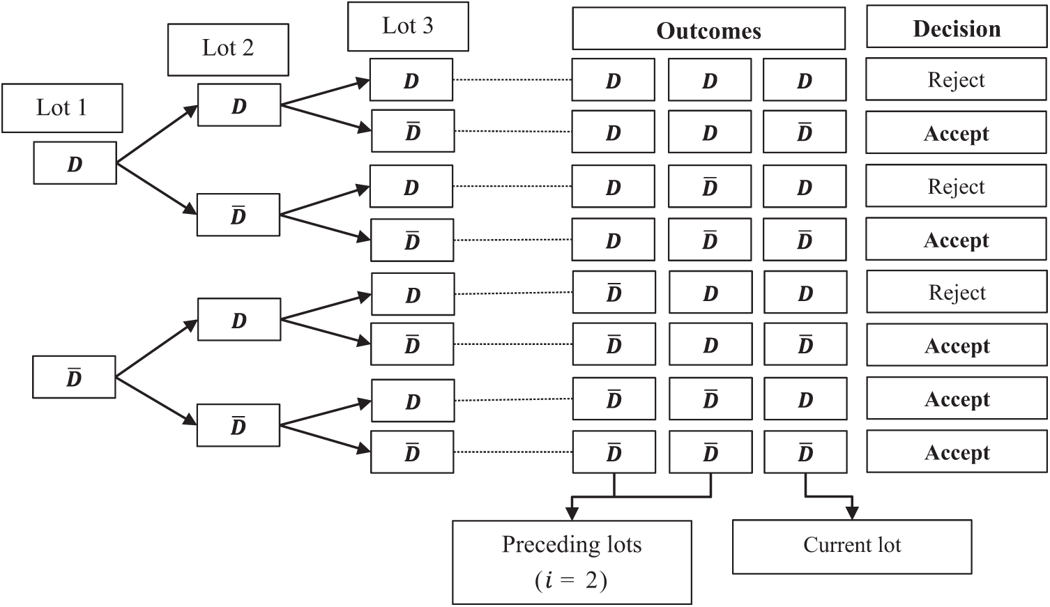
Figure 2: Tree diagram for the proposed sampling plan

In attribute acceptance sampling, lot inspection is based on the number of defectives (discrete variable). The procedure of GChSP for i=2, is illustrated through a tree diagram, represented in Fig. 2, where defective and non-defective products are denoted by D and D¯, respectively. From Fig. 2, for i=2 it can observed that GChSP has five acceptance criteria (AC) {DDD¯,DD¯D¯,D¯DD¯,D¯D¯D,D¯D¯D¯}. Here {DDD¯,DD¯D¯,D¯DD¯,D¯D¯D¯} concern with the current lot, hence the probability of lot acceptance is P0 and {D¯D¯D} has a probability of lot acceptance P0P0P1. Finally in the group chain, the probability of lot acceptance can be written as:

L(p)GChSP=P0+P0P0P1 (1)

L(p)GChSP=P0+P1(P0)2 (2)

The general expression for i=2 is like the operating characteristics (OC) function of ChSP-1 given by Dodge [10].

L(p)GChSP=P0+P1(P0)i (3)

For the average number of defectives, consider Poisson distribution with mean μ=np and n=r∗g, to achieve the probability of lot acceptance for zero and one defective product which are respectively:

P0=e−(r∗g)p, (4)

P1=(r∗g)pe−(r∗g)p. (5)

After replacing Eqs. (4) and (5) in Eq. (3), we get:

L(p)GChSP=e−(r∗g)p{1+(r∗g)pe−(r∗g)pi}. (6)

Let us consider gamma distribution as a suitable prior for the Poisson distribution [26,27], with pdf:

f(p)=tsΓ(s)ps−1e−tp, (7)

where shape parameter, s>0 and rate parameter, t>0 with mean μ=st under the proposed sampling plan. For the average probability of lot acceptance, the general expression used in Bayesian is as follows:

P¯=∫0∞L(p)f(p)dp. (8)

After replacing Eqs. (6) and (7) in Eq. (8) and then from simplification we get:

P¯=tsΓ(s)[Γ(s)(r∗g+t)s+(r∗g)Γ(s+1)(r∗g∗(1+i)+t)s+1], (9)

P¯=(tr∗g+t)s+(r∗g)sts(r∗g(1+i)+t)s+1. (10)

Upon substituting mean μ=st in Eq. (10) and simplifying:

P¯=(srgμ+s)s+rgμss+1(rgμ(1+i)+s)s+1. (11)

Further simplification of Eq. (11), for s=1,2,3 gives:

P¯=1(rgμ+1)+rgμ(rgμ(1+i)+1)2, (12)

P¯=4(rgμ+2)2+8rgμ(rgμ(1+i)+2)3, (13)

P¯=27(rgμ+3)3+81rgμ(rgμ(1+i)+3)4. (14)

It is to be noted that Newton’s approximation is employed in Eqs. (12)–(14) to find the quality regions of BGChSP, where μ is used as a point of control by reducing P¯. Tab. 1 presents the average number of defectives for the specified values of shape parameter s=1,2,3; the number of testers r=2,3,4 and number of preceding lots i=1,2,3,4. Operating ratios for different values of consumer’s risk and producer’s risk are presented in Tab. 2.

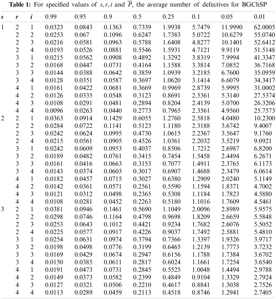
Example 1: In Tab. 1, for s=1,r=2, i=3 and P¯=0.50 the corresponding value of the average number of defectives is 0.5788 and for s=2,r=3 and i=4, the corresponding value is 0.3017. From Tab. 1, it can be concluded that as the values of s,r and i are increased the average number of defective products decreases.

3.1 Designing Sampling Plans for Given AQL and LQL

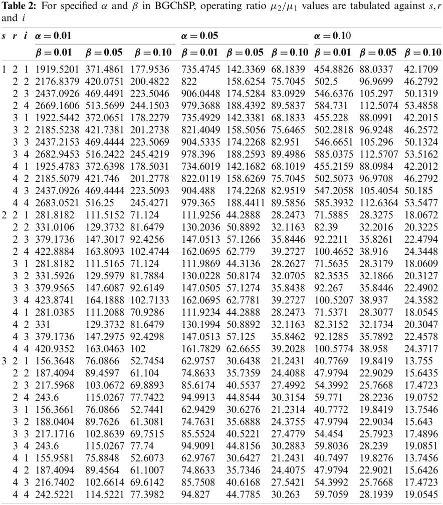
For the selection of BGChSP, Tabs. 1–2 are used for specified AQL, LQL, α and β by using the following three steps: (i) construct a plan for the given points (AQL, 1−α) and (LQL, β), then compute the desired operating ratio; (ii) from Tab. 2, find the value of the operating ratio that is equal to or just less than the desired operating ratio in the desired columns for α,β; (iii) obtain the corresponding values of s,r,g and i, from Tab. 1 for the corresponding located value of the operating ratio given in Tab. 2.

3.2 Construction of Quality Regions

3.2.1 Probabilistic Quality Region (PQR)

In this quality region, the product is accepted with the maximum probability of 0.95 and minimum probability of 0.10, where 0.95 corresponds to (AQL, 1−α) and 0.10 corresponds to (LQL, β). In other words, PQR (R1) is exactly the conventional setting of AQL=μ1 and LQL=μ2. In Fig. 3, we can see the PQR lies between μ1<R1<μ2.

The range of probability is R1=μ2−μ1 which is derived from the equation of the average probability of acceptance Eq. (11). This Eq. (11) is used in the same way to find AQL, LQL and operating ratios represented in Tab. 3.

3.2.2 Indifference Quality Region (IQR)

In IQR, the product is accepted with maximum and minimum probabilities 0.95 and 0.50, that correspond to (AQL, 1−α) and (LQL, β) respectively. Hence, R0=μ0−μ1 is the range of IQR and lies in the interval μ1<R0<μ0. This is obtained from the average probability of acceptance Eq. (11).

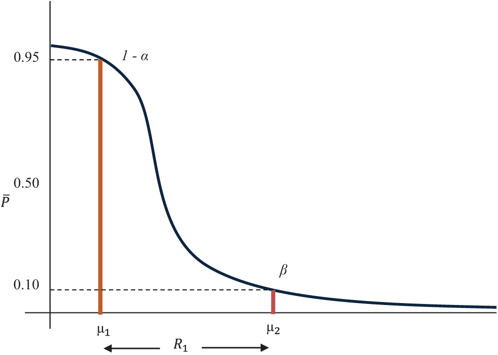
Figure 3: OC curve with pair of coordinates for PQR

Example 2: Let s=1 at α=0.10 and β=0.05, μ1 = 0.008 and μ2 =0.90, then the operating ratio μ2μ1 = 112.5. From Tab. 2 the value 112.6364 with design parameters s=1,r=4,i=4 is approximately equal to this calculated operating ratio. With the same design parameters s=1,r=4 and i=4 from Tab. 1, the corresponding value of gμ1=0.044. The number of groups can be obtained by gμ1μ1=5.5-the required minimum number of groups is approximately 6 in order to get the required operating ratio. For this operating ratio, the parametric values are s=1,g=6,r=4,i=4 at α=0.10 and β=0.05. Also, the corresponding value of AQL is μ1=0.008 and LQL is μ2=0.9.

3.3 Selection of Sampling Plans

For different values of s and r in Tab. 3 the operating ratio T is given, i.e., T=μ2−μ1μ0−μ1=R1R0, where R1 and R0 are used to characterize the sampling plan. Operating ratio T=R1R0 can be found for any given values of PQR (R1) and IQR (R0). First we find the value in Tab. 3 under the column of T, that is equal to or just less than the specified ratio. Then for this operating ratio, the corresponding parameters values can be determined for s,r and i in BGChSP.

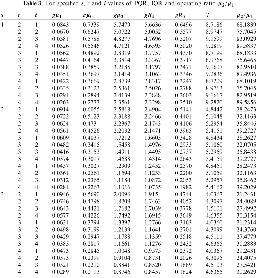
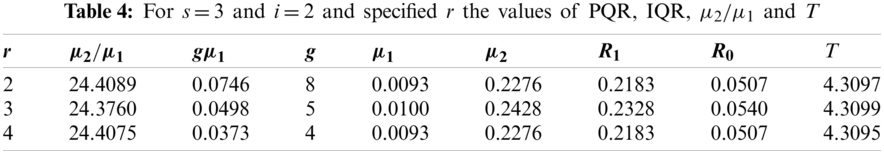
Example 3: At α=0.05 and β=0.1 let μ1=0.01 and μ2=0.25, then the operating ratio will be μ2/μ1=25. From Tab. 3 for this operating ratio, the nearer values are 24.4089, 24.376 and 24.4075. The nearest values of PQR and IQR corresponding to s=3 and i=2 will be found based on the minimum number of groups g.

Hence from Tab. 4, through quality region the required plan has parameters s=3, g=5 and r=3. The nearest values of PQR and IQR are R1=0.2328, R0=0.0540 and T=4.3099 corresponding to s=3, g=5, r=3, i=2 and μ1=0.0107.

4  Conclusion

In this acceptance sampling plan, both risks are used to balance the expected losses for the consumers and producers. The presented work is limited to BGChSP and estimate PQR and IQR for the specified producer’s and consumer’s risks. This research gives the idea to estimate an interval of average number of defectives for prespecified design parameters. Quality interval sampling plans have wider potential applications in the industry to ensure that the product or process complies with a higher quality standard. Thus, quality interval sampling could be useful for outlining product quality, planning, and quality control arrangements that are ready for electronic industrial applications. Many electronic components such as transport electronics systems, wireless systems, global positioning systems, and computer-supported and integrated manufacturing systems can be evaluated by using the proposed plan. Many other distributions and other quality and reliability characteristics can be explored in the future.

Funding Statement: This research was supported by the Ministry of Education (MOE) through Fundamental Research Grant Scheme (FRGS/1/2020/STG06/UUM/02/2), S/O Code 14884.

Conflicts of Interest: The authors declare that they have no conflicts of interest to report regarding the present study.

This work is licensed under a Creative Commons Attribution 4.0 International License, which permits unrestricted use, distribution, and reproduction in any medium, provided the original work is properly cited.