Computers, Materials & Continua DOI:10.32604/cmc.2022.019559
Article

Neural Network and Fuzzy Control Based 11-Level Cascaded Inverter Operation

Buddhadeva Sahoo1,*, Sangram Keshari Routray2, Pravat Kumar Rout2 and Mohammed M. Alhaider3

1Department of Electrical Engineering, Siksha ‘O’ Anusandhan University, Odisha, 751030, India
2Department of Electrical Electronics Engineering, Siksha ‘O’ Anusandhan University, Odisha, 751030, India
3College of Engineering at Wadi Addawaser, Prince Sattam bin Abdulaziz University, 11991, Saudi Arabia
*Corresponding Author: Buddhadeva Sahoo. Email: buddhadeva14@gmail.com
Received: 17 April 2021; Accepted: 05 June 2021

Abstract: This paper presents a combined control and modulation technique to enhance the power quality (PQ) and power reliability (PR) of a hybrid energy system (HES) through a single-phase 11-level cascaded H-bridge inverter (11-CHBI). The controller and inverter specifically regulate the HES and meet the load demand. To track optimum power, a Modified Perturb and Observe (MP&O) technique is used for HES. Ultra-capacitor (UCAP) based energy storage device and a novel current control strategy are proposed to provide additional active power support during both voltage sag and swell conditions. For an improved PQ and PR, a two-way current control strategy such as the main controller (MC) and auxiliary controller (AC) is suggested for the 11-CHBI operation. MC is used to regulate the active current component through the fuzzy controller (FC), and AC is used to regulate the dc-link voltage of CHBI through a neural network-based PI controller (ANN-PI). By tracking the reference signals from MC and AC, a novel hybrid pulse width modulation (HPWM) technique is proposed for the 11-CHBI operation. To justify and analyze the MATLAB/Simulink software-based designed model, the robust controller performance is tested through numerous steady-state and dynamic state case studies.

Keywords: Ultra-capacitor; 11-level cascaded H-bridge inverter; hybrid energy system; modified perturb and observer; neural network-based PI; fuzzy controller

1  Introduction

Due to the excess energy demand, there is a requirement for high power quality (PQ) microgrid stations for reliable power supply. As a solution, the research has been focused on the development of storage devices (SD), hybrid energy system (HES) integration, maximum power point (MPP) operation, multi-level inverter (MLI) operation, and robust control strategy [1,2]. In [3,4], it is found that the total life cycle cost of the standalone microgrid system is decreased by maintaining the PQ with the integration of HES. In [5,6], different MPP techniques are proposed to track maximum power from the HES. However, looking at the complexity, the conventional MPP techniques lag to track maximum power. Therefore, there is a necessity to design an improved MPP strategy for facilitating a reliable power supply.

To improve the PQ and PR of the low, medium, and high-power HES applications, multi-level inverter (MLI) topologies such as a diode-clamped inverter (DCI) [7], flying capacitor inverter (FCI) [8], and cascaded H-bridge inverter (CHBI) [9] play an important role. The capability of generating multilevel voltage outputs facilitates the direct integration of the HES to the grid without requiring additional devices [10]. As compared to conventional inverters, MLI provides attractive features like increased voltage levels, smaller filter size, lower electromagnetic interfaces (EMIs), and lesser harmonic currents [11]. However, compared to CHBI, the DCI and FCI require more components such as a diode, and capacitors to generate more voltage levels and lesser harmonic current. To generate more voltage levels and facilitate HES integration, CHBI is widely accepted due to the availability of more dc voltage sources [12]. Considering the advantages of CHBI, there is a necessity to develop a novel CHBI for improving the PQ and PR operation for a HES integration.

Due to the increased cost and less durability of SD, different control approaches are suggested in [13,14] to reduce additional power injections and the burden of HES. Later on, researchers decrease the cost of the SD with an increase in the life cycle [15]. However, due to the uncertainty in HES, uninterruptable power supply (UPS), flywheel, battery, capacitors, and ultra-capacitors (UCAPs) are required at the dc-terminal of the active power filter for compensating the voltage fluctuations [16,17]. A comparative study between all of the SDs are presented in [18]. In [19], a novel energy scheduling method is proposed to overcome the uncertainty present in the generation sector. However, this is silent about the design and selection of battery factors. In addition to that, the paper is only considered the generation side uncertainty. In [20], a novel management approach is proposed to reduce the electricity bill by properly managing the electric supply. However, this paper is silent about the PQ and size of the battery. Researchers are giving more efforts to provide active power support during unbalanced conditions by integrating the SD with the active power filter-based inverters [21]. By comparing all the SDs, it is found that UCAP based SD provides better active power support in ms to μs time range [16,18,21]. Therefore, looking at the UCAP characteristics like less energy and high-power concentration, it is widely accepted [18,21]. Moreover, an increasing number of charging/discharging cycles make the installation easier as compared to the battery of the same size. Therefore, considering the advantage of UCAP, there is a necessity to integrate the UCAP based SD with a CHBI inverter.

Due to the excess application of sensitive load, the working condition of CHBI depends upon the speed and accurate extraction of the harmonic component through the proposed controller action [20]. As a solution, different fast and accurate extraction control techniques such as the conventional PQ approach, adaptive filters, signal processing, optimization technique, morphological techniques, and ANN techniques are developed [21]. Recently, ANN-based techniques draw attraction for CHBI operation [22]. In [23], by using an Adaline network, the Fourier coefficient of the desired signal is computed and in [24], ANN is trained through a backpropagation and genetic algorithm technique. A Hopfield network [25] and a Kalman filter [26] based technique, is suggested for the computation of frequency and the harmonic component. In addition to that, an additional PI controller is used to compute the dc-link voltage of the system. The predictive control techniques are only focusing on the extraction of harmonic components for active filter operation. However, the active power filter and power flow of the system is not only depending upon the harmonic extraction. In [27,28], single-phase grid-connected and standalone solar system control approaches are proposed for appropriate power computation. The aforementioned control techniques are based on the conventional PI controllers for the control design. However, due to the lack of an appropriate method, different trial and error methods are used to compute the PI controller gain parameter. In [29], a continuous mixed P-norm (CMPN)-based adaptive PI regulator is suggested for similar applications. In [30], the fractional-order PI regulator is proposed for optimum results through the controller. In [31], the particle swarm optimization algorithm (PSO) is suggested for tuning the regulator parameters for better performance. However, these controllers some extent enhances the robustness and performance of the controller for appropriate power extraction. Therefore, there is a necessity to develop an HPWM technique to regulate the dc-link voltage and power flow of the HES.

The major contribution of the proposed approach is presented below.

•   To regulate the low-quality power, MP&O technique-based boost converter is used for solar and wind converter respectively.

•   A novel 11-level CHBI with a reduced number of switches is designed by combining a 3-level solar and 5-level wind inverter.

•   To provide independent active power support, UCAP is integrated with the solar dc-link capacitor through a bidirectional converter. A novel current control strategy is proposed by properly sensing the dc-link voltage of the solar inverter and the robustness of the controller is tested through different stability results.

•   To develop a robust controller for 11-CHBI, the controller is divided into two specific controllers such as main controller (MC) and the auxiliary controller (AC).

•   To improve the PQ, PR, and stability, the MC is designed by considering 7 * 7 fuzzy controller, and AC is designed by considering an ANN-PI controller.

•   To make the controller more robust, a novel HPWM is proposed for the 11-CHBI operation.

2  System Configuration and MPP Operation

Fig. 1 illustrates the overall block diagram of HES comprised with UCAP and single-phase 11-CHBI. 11-level CHBI is designed by combining 2-level Solar and a 5-level Wind inverter. To compensate the voltage disturbances, UCAP is connected to the dc-link solar capacitor. The switches Sw1 and Sw2 are integrated for regulating the wind, solar, and intermittent loads. As illustrated in Fig. 1, a single-phase non-linear load is integrated with the HES. At different environmental conditions, the locus of MPP changes for a wider range [4]. Specific to the solar and wind-based HES, the PR issues are more complex to handle as the MPP depends upon environmental conditions.

Figure 1: Block diagram of the projected system configuration

Researchers suggest different tracking methods to improve PR by generating maximum power [1,2]. From the literature, it is concluded that few of the research perform well in the case of the steady-state condition [3,4] and also some of the research performs well in the case of dynamic state conditions [12]. Generally, the conventional P&O technique (CP&O) and Hill-Climbing techniques are widely used for HES due to their low cost, simpler design, and easy implementation [21]. In the case of solar, the MPP method tracks the voltage and current, and in the case of a wind turbine, the MPP method tracks the speed and torque. In this proposed approach, for tracking optimum power and improve the PQ, the MP&O technique is used for both solar and wind systems. The detailed analysis regarding the MP&O method for both solar and wind systems is discussed in [32,33]. By using MP&O, the obtained maximum power results under the change in environmental and constant load conditions are illustrated in Figs. 2a–2d.

3  11-CHBI Topology

To integrate HES with the grid, a novel 11-CHBI is proposed. For facilitating 11 output voltage levels, a 3-level solar inverter is cascaded with the 5-level wind inverter. By cascading two inverters, the 11-CHBI inverter offers reduced dc-link voltages (two) and switch operations. The undertaken components, switching sequences, and the dc-link capacitor ratings are presented below. Wind H-bridge inverter (WHBI) is designed by combining an auxiliary circuit and a single-phase inverter. The auxiliary circuit consists of four diodes (D1–D4), and an operating switch (SL) is incorporated between them [12–16], and the single-phase inverter consists of four operating switches (S5–S8). In addition to that, four operating switches (S1–S4) are used to design the solar H-bridge inverter (SHBI). The dc-link capacitor (C2 and C3) voltage of WHBI is two times the dc-link capacitor (C1) voltage of the SHBI (i.e., 2 Vdc2 = 2 Vdc3 = Vdc1).

Therefore, the dc-link voltage of the WHBI (Vw) is four times the dc-link voltage of the SHBI (Vs) [12]. Generally, the WHBI generates the voltage level Vw = 2 k + 1 level, and the SHBI generates Vs = Vdc1. Here ‘k’ denotes the number of capacitors used in the WHBI. By combining the two-inverter output, as a total ‘4 k + 3’ system voltage (VT) levels are produced. The SHBI generates 3-level output voltages as (±Vdc1, 0) and the WHBI generates 5-level output voltages as (±4Vdc1,±2Vdc1, 0). The switching states and voltage levels of the proposed 11-CHBI are presented in Tab. 1. The equivalent operational circuit diagrams with six operating cases are illustrated in Figs. 3a–3f.

Figure 2: Characteristics curves of solar and wind system (a) Power (W) vs. Voltage (V) and (b) Current (A) vs. Voltage (V) (c) Wind speed vs. Power (d) Turbine speed vs. Power

Case-1: As illustrated in Fig. 3a, both S5 and S8 are at ON condition. To make continuous conduction of the current, C2 and C3 are discharged together through S5, filter, utility, and S8. The output voltage of the wind inverter is 4 Vdc during this period.

Case-2: As illustrated in Fig. 3b, both SL and S8 are at ON condition. To make continuous conduction of the current, C3 is discharged through D1, SL, D4, utility, S8, and filter. Due to the discharge of C3, the output voltage of the wind inverter is 2Vdc during this period.

Case-3: As illustrated in Fig. 3c, both S5 and S6 are at ON condition. To make continuous conduction of the current, the current passes through utility, filter, S5, and S6. As C2 and C3 are not in discharging mode, the output voltage of the wind inverter is zero during this period.

Case-4: As illustrated in Fig. 3d, both S7 and S8 are at ON condition. To make continuous conduction of the current, the current passes through utility, filter, S6, and S8. As C2 and C3 are not in discharging mode, during this condition also the output voltage of the wind inverter is zero (similar to Case-3).

Case-5: As illustrated in Fig. 3e, both SL and S6 are at ON condition. To do continuous conduction of the current, C2 is in the discharged mode condition through a filter, D3, SL, D2, S6, and utility. Due to C2 discharge, the output voltage of the wind inverter is negative (−2 Vdc) during this period.

Case-6: As illustrated in Fig. 3f, both S6 and S7 are at ON condition. To make continuous conduction of current, C2 and C3 both are at discharging condition through the filter, S7, S6, and utility. The output voltage of the 5-level inverter is negative (−4 Vdc) during this period.

Figure 3: Operational equivalent circuit of a five-level CHBI. (a) Case-1 (b) Case-2 (c) Case-3 (d) Case-4 (e) Case-5 (f) Case-6. *Red line indicates the conduction sof switches according to the cases

4  UCAP Based Energy Storage Device

To provide active power support during voltage unbalance conditions, the detailed explanation regarding the proposed UCAP control strategy is illustrated in Fig. 4. Due to the change in the voltage profile of the UCAP at the discharging condition, UCAP is connected with the dc-link capacitor of SHBI through a bidirectional dc-dc converter.

In the suggested approach, the rating of three series-connected UCAPs (each having 48 V, 165 F) (BMOD0165P048) manufactured by Maxwell Technologies is considered. As a result, the total capacity of the UCAP becomes 144 V and the reference voltage (Vdc, ref) is chosen as 260 V. Instead of considering the dump load discussed in [34], the output of the bidirectional converter consists of a load (RL) of about 215.3 Ω is taken to prevent the no-load condition. A detailed explanation for a similar approach is presented in [35].

During voltage sag and swell conditions, depending on the duration and depth of the sag and swell, the dc-dc converter gives and absorbs power respectively. For better performance of the UCAP, the voltage range of UCAP is regulated by the proposed controller. When the UCAP voltage is between 72 to 144 V, the bidirectional converter behaves as a boost converter, and the output voltage of the converter is normalized at 260 V. Similarly, when the voltage is less than 72 V, it operates as a buck converter and it draws power from the grid to charge the UCAP. The proposed average current control technique is illustrated in Fig. 4.

Figure 4: Operating conditions of the UCAP

The dc-link voltage of the solar module (Vs) is affected due to the voltage sag and swell condition. As illustrated in Fig. 4, to generate a minimum error (Vdc, e), the output voltage of the bidirectional converter (Vo) is compared with the Vs. After generating Vdc, e, it is compared with the Vdc, ref to generate the appropriate dc-link voltage (Vdc-link). To generate the appropriate reference UCAP current (Iucap, ref), Vdc-link is passed through the voltage compensator CV(s) [21,23].

The complete control structure of the dc-link voltage regulation scheme is illustrated in Fig. 5. Any type of grid, load, and input fluctuations are specifically affecting the dc-link voltage of the inverter. Therefore, the proper control of dc-link voltage is very much important to improve the stability of the system. The dc-link voltage control stability is tested and justified through different Bode and Nyquist plot results. From the illustrated Fig. 5, the open-loop transfer function of the compensator is obtained as

G(s)=Kp+Kis (1)

From Fig. 5, the open-loop (Gopen(s)) and closed-loop (Hclosed(s)) transfer function of is developed as.

Gopen(s)=(Kp+Kis)(1Cdcs) (2)

Hclosed(s)=(1Cdc)×(Kps+Kis2+KpCdcs+KiCdc) (3)

Figure 5: Complete structure of dc-link voltage regulation

From Eq. (3), it is identified as Hclosed(s) is a second-order system. From Eq. (3), the damping ratio (ξ) and bandwidth (ωc) of the proposed compensator are computed as.

2ξωc=KpCdc⇒Kp=2ξCdcωc (4)

ωc2=KiCdc⇒Ki=Cdcωc2 (5)

The Bode response of the open-loop function of the voltage compensator at different bandwidth (ωc) is demonstrated in Fig. 6a. To comprehend a good rapport between the static and dynamic responses, the damping fraction (ξ) should lie between 0.4–0.8. Fig. 6a shows that at ωc=458, the system offers a much linear output as compared to other ωc values. By using ωc=458 and dc-link capacitor (Cdc) of the CHBI, the Kp and Ki constraints are computed as 3.15 and 1000 (larger value) respectively. By using the above-computed values the voltage compensator equation becomes.

CV(s)=3.15+1000s (6)

The stability of the closed-loop voltage compensator is evaluated by considering the obtained Kp and Ki constraints through Bode and Nyquist responses. The Bode and Nyquist response of the closed-loop system are illustrated in Figs. 6b and 6c, respectively.

Similarly, the current compensator values CI(s) are computed. The actual UCAP current (Iucap) is compared with the Iucap, ref, to generate the current error (Iucap, e). To linearize the Iucap, e, it is passed through the current compensator CI(s) and used for pulse generation by using PWM techniques. During the boost mode, the converter discharges power into the grid, and Vo tends to decrease even below the reference voltage (Vdc, ref), which makes the error and Iucap, ref positive. Similarly, during buck mode, the converter absorbs power from the grid, and Vo tends to increase even above the Vdc, ref, which makes the error, and Iucap, ref negative. The CI(s) is represented as:

CI(s)=1.68+23.85s (7)

Figure 6: Open-loop (a) Bode response at different band-width, closed-loop (b) Bode response, (c) Nyquist response

5  Control Strategy

To operate 11-CHBI, the proposed control strategy is divided into two sections such as system current control (SCC) and inverter switching control (ISC). SCC is proposed to regulate the grid parameters and dc-link voltage inverter by eliminating the nonlinearity. In addition to that, ISC is proposed to generate appropriate pulses for SHBI and WHBI respectively. The related explanations about the proposed strategies are presented below.

5.1 System Current Control (SCC)

As illustrated in Fig. 7, the SCC strategy is based upon a two-way conversion topology as the MC and AC. MC is used to generate the modulating signals (Msignal) for 11-CHBI by regulating the related power and voltage of the CHBI through FC. In addition to that, for generating the appropriate modulation signal for the respective inverters (Ms and Mw) are achieved by regulating the dc-link voltage of CHBI through an ANN technique. A detailed explanation of the control design is presented below.

Figure 7: Control system diagram by showing both of the controller performance

5.1.1 MC Performance

The key objective of this controller is to adjust the sum of the dc-link voltage (Vw and Vs) of both wind and solar inverter to the preset desired value (VT), by which the 11-CHBI generates an accurate output voltage and the sinusoidal output current.

The corresponding power equation can be written as:

Pe=(Pw+Ps)−PLoad+Pgrid (8)

Pe=Vrms×Irms=Vrms×I^p2 (9)

where ‘Pw’, and ‘Ps’ are the power generated from the wind and solar system respectively. Pgrid and PLoad are the grid power and load power respectively. Depending upon the generation and demand of the load and grid, the extra power (Pe) is computed. Neglecting the losses (PL), the peak currents Ip and I¯p can be expressed as:

Ip=(Pe)×2Vrms (10)

VT−(Vdc,w+Vdc,s)=Ve (11)

The Ip current is passed through an FC, to generate the reference current (I^p) by eliminating the harmonic component generated from the nonlinear load. To generate accurate I¯p, the generated Ve passes through the FC as shown in Fig. 7. The controller consists of two input constraints named actual and changes in constraints. Each input constraint contains seven linguistic variables named as large positive (LP), medium positive (MP), small positive (SP), large negative (LN), medium negative (MN), and small negative (SN). However, the FC is planned by using 49 rules as demonstrated in Tab. 2.

The total peak current Ip is calculated as:

Ip=I^p+I¯p (12)

The major objective behind this control design is to synchronize the HES to the grid and balances the output current. As shown in Fig. 7, to generate a sinusoidal reference (sin⁡ωt), the grid voltage is passed through the Phase Locked Loop (PLL). By multiplying the ‘Ip’ with sin⁡ωt, a sinusoidal current reference is generated. By using the FC, the MC generates the Msignal by which the AC is operated.

5.1.2 Auxiliary Control (AC) Performance

The basic purpose of AC is to regulate the dc-link voltage of the respective solar and wind inverter. As illustrated in Fig. 7, Vs and Vw are compared with the reference voltage of Vs, ref, and Vw, ref respectively. Vs, ref, and Vdcw, ref is calculated as:

Vs,ref=VT5 (13)

Vw,ref=4×VT5 (14)

To eliminate the uncertainty, the respective error in the dc-link voltage is passed through the ANN-PI controller as shown in Fig. 8. To reduce the circuit complexity and computational burden, a single layer ANN is used. The input vector (u) such as Vdc and Vdc, ref fed into the state generator as indicated in Eq. (15). In this approach, the error voltage ‘Ve’ and its gradient are selected as the states of the system for faster estimation.

u=|Vdc,refVdc|T (15)

State generator generates the states (a1 and a2) and represented as:

a1=Ve(n) (16)

a2=δa1δn (17)

where Ve(n)=Vdc,ref−Vdc(n). The error in output Z (n) is calculated as:

Z(n)=VO(n)−VO(n−1) (18)

Figure 8: ANN-based peak value predictor block diagram

The output voltage VO(n) is sent to the output state to calculate ‘Iα’. The controlling signals are generated by the neuron cell through interrelated gatherings [21] and represented as:

u(n)=u(n−1)+∑j=12Wj(n)aj(n) (19)

where ‘Wj’ is denoted as the weight of the system. In this test system, the neuron is operated by Hebb’s rule [21,22]. The change of weight for nth instant is expressed as:

Wj(n+1)=(1−c)Wj(n)+ηrj(n) (20)

rj(n)=Z(n)u(n)aj(n) (21)

where rj, η, and c denote as the progressive signal, Hebb’s learning ratio, and constant term respectively. Substituting Eqs. (20) and (21) in Eq. (19), the corresponding equations become:

ΔWj(n)=Wj(n+1)−Wj(n)=−c(Wj(n)−ηZ(n)u(n)aj(n)/c) (22)

where ΔWj(n) denotes as the weight change at nth instant. The weight of the neuron is optimized by following Hebb’s learning rule known as covariance algorithm and can be represented as:

ΔWj(n)=Fj(Y(n),aj(n)) (23)

where Fj (*) denotes as the post and presynaptic function and ‘Y’ denotes as each neural output. By differentiating Fj (*), it becomes:

δFjδWj=Wj(n)−ηcZ(n)u(n)aj(n) (24)

From Eq. (24), weight change for nth instant can be represented as follows:

ΔWj(n)=−cδFj(n)δWj(n) (25)

By updating the values of Wj(n), the constant parameters of the PI controller are optimized. The base values of the PI controller parameter are generated from the following Eq. (41).

IG⟨CdcVdc,ref3KpLF (26)

IG≤VGKp2RFKp+LFKi (27)

The parameters IG, VG, and Vdc,ref denote as the grid voltage, grid current, and reference voltage respectively. To find the initial assumption of the constant parameters of the PI controller, all the ac quantities in Eqs. (26) and (27) are expressed in RMS values. The weights are selected by using the negative slope values of the functions Fj (*). For the PI current controller, the weights can be expressed as:

W1(n+1)=W1(n)+ηIZ(n)a1(n) (28)

W2(n+1)=W2(n)+ηPZ(n)a1(n) (29)

By using Eqs. (24) and (25), the parameters of Eqs. (28) and (29) are optimized. At the initial condition, the quick estimation of the compensating currents is done by using a set of controller weights. The above initial weights of the controller are set by offline training of the ANN. The weights are subsequently optimized by the Eqs. (28) and (29) to adjust the dc-link voltage. The generated output of the ANN is multiplied with the Msignal, to produce the modulating signals for the wind and solar inverters (Mw and Ms) respectively.

The stability of the ANN-PI-based control system is proved through different Bode and Error plot results. By using the PI control approach, the voltage stability is decreased as illustrated in Fig. 9a. Different PI parameter constraints are derived at different state conditions of DFIG. However, by using the proposed ANN-PI-based controller, the open-loop transfer function of the undertaken system gives better stability results as illustrated in Fig. 9a. It is found that at 21.9 dB gain margin (at 16.4 rad/s) and 65.8 deg (at 2.93 rad/s), the ANN-PI-based open-loop transfer function gives faster and more stable results. In addition to that, to give a better justification, the error in the voltage component is also illustrated in Fig. 9b. Fig. 9b illustrates that the proposed approach provides a faster stability response with 0.448 s rise time and 1.22 settling time as compared to the traditional approach. Looking at Figs. 9a and 9b, the above phase margins and gain margin values are used to compute the PI values and by using the PI parameters, the closed-loop stability response of the system is illustrated in Fig. 9c. This justifies the need for the proposed controller during complex system applications with improved stability.

5.2 Inverter Switching Control (ISC)

The HPWM technique is incorporated into the AC for generating appropriate pulses for the respective inverter. A detailed explanation regarding the proposed technique is illustrated below. The total reference waveform ‘Ur’ is represented as:

Ur=Bsin⁡(ωt) (30)

where ‘B’ denotes the peak value of the reference waveform and calculated as:

B=N−12 (31)

where N (N = 11,15, 19, 23, etc.) denotes the inverter output voltage level. In the present study as the N is considered as 11, the peak value ‘B’ is computed according to Eq. (31) as 5. Eq. (30) can be represented as:

Ur,s=Ur5 (32)

The switching sequences for both solar and wind inverters are described separately in the following sections.

5.2.1 Solar Inverter Switching Sequences

To operate the solar inverter, the reference signals (S01 and S02) are produced by the following expressions:

T=1,if Ur⟩00,if Ur⟨0 (33)

Vwind,expected=[round(|Ur,s|0.4)×0.4×T]+[round(|Ur,s|−0.4)×0.4×T] (34)

The reference signals (S01, and S02) for operating the switches of the solar inverter can be expressed as:

S01=5×(Ur,s−Vwind,expected) (35)

S02=1−[5×(Ur,s−Vwind,expected)] (36)

Figure 9: ANN-based peak value predictor block diagram. (a) Comparative open loop transfer function Bode response (b) Voltage error (c) Closed loop transfer function Bode response

Figure 10: Switching pulses logic diagram of solar inverter

The corresponding logic diagram of Eqs. (35) and (36) is illustrated in Fig. 10. Eq. (33) represents a simple zero-crossing detector, Eq. (34) represents the output expected for the wind inverter, and Eqs. (35) & (36) represent the mathematical expression for the solar inverter reference signals. For higher-level output voltage, the above equations are needed by modifying the peak values of ‘B’.

5.2.2 Wind Inverter Switching Sequences

To produce the reference signals for the wind inverter, the first step is to produce the reference waveform (Vwind,r) for the wind H-bridge inverter. This can be computed as:

Vwind,r=round(|Ur,s|0.4) (37)

The next step is to produce many reference signals (Kn) from the above reference waveform to operate the auxiliary circuit and switches of the wind H-bridge inverter and can be calculated as:

Kn=1,if Ur⟩n0,if Ur⟨n (38)

where n = 1, 2, 3…. Z.

The ‘Z’ is calculated as:

Z=N−114+2 (39)

The auxiliary switch is varying from ‘1’ to ‘X’ numbers depending upon the level of generation.

By applying N = 11, in Eq. (34) the value of ‘Z’ becomes 2. This indicates there are two conditions to generate the operating signals for the wind inverter and is represented as:

K1=1,if Uwind,r⟩10,if Uwind,r⟨0 (40)

K2=1,if Uwind,r⟩20,if Uwind,r⟨0 (41)

For 11-level operation the main operating switches (S5, S6, S7, and S8) of the wind inverter are operated as per the equations given below [7]:

S5=|K¯1+K¯2|×T (42)

S6=|K1+T¯|+|K¯1×T| (43)

S7=|K¯1+K2|×T¯ (44)

S8=|K1+T|+|K¯1×T¯| (45)

where ‘+’ and ‘×’ are used for the logic OR and logic AND operations respectively.

The logic diagram of the reference signal is illustrated in Fig. 11. After generating the reference signals for the main switches of the wind inverter; the next step is to find the reference signal for the auxiliary switch. The number of auxiliary switches (N*A) and the reference signals for the conduction of switches are calculated as follows.

N∗A=N−114+1 (46)

Figure 11: Switching pulse logic diagram of wind inverter

From [7], the switching pulses for the auxiliary circuit are calculated as:

1A=((K1⊕K2)×T¯)+((KZ−1⊕KZ)×T) (47)

N∗A=((K1⊕K2)×T)+((KZ−1⊕KZ)×T¯) (48)

By using the above concept, other reference signals are calculated for the respective auxiliary switches. The symbol ⊕ denotes the logical XOR operation. To generate the 11-level output voltage, the auxiliary switch is calculated as:

N∗A=N−114+1=1 (49)

Therefore, the reference signal for the auxiliary circuit of 11-level CHBI is represented as:

1A=((K1⊕K2)×T¯) (50)

The different possible reference signals are generated for the switching operation of the 11-CHBI.

6  Result Analysis

The performance of the proposed control strategies with the 11-CHBI operation is tested under steady-state and dynamic state conditions. The dynamic state conditions are achieved during the fall in solar and wind power and change in voltage level. In addition to that, a comparative study section is also presented by showing the harmonic percentage improvement over other conventional strategies.

Condition.1 Steady-State Condition

Case-1: MPP Operation

This section demonstrates the performance analysis of MP&O based MPP technique under a sudden change in environmental conditions for solar and wind systems as illustrated in Fig. 12. Fig. 12a illustrates the simulation results of a 180 W solar module at rapid change in irradiance (G) conditions at 25∘C. To show the effectiveness of the controller, the irradiance is changed from 1000–100–1000–600–800 W/m2 at a time interval 0–0.3–0.5–0.7–0.9–1 s respectively. As per the set condition, the proposed MP&O tracks maximum power as illustrated in Fig. 12a. Fig. 12a shows that solar power is changed from 180–100–180–103–140 W respectively. The obtained power results are matched with the MPP of the P-V and I-V characteristic results as illustrated in Figs. 2a–2b. Fig. 12b illustrates the simulation results of a 2kW wind system at a rapid change in wind speed (n) conditions by using the MP&O technique. To show the effectiveness of the controller, the speed is intentionally changed from 6–6–8–8–10–10–6–6 m/s during a time interval of 0–0.5–1–1.5–1.5–2–2.5–3 s respectively. As per the set condition, the proposed MP&O tracks maximum power as illustrated in Fig. 12b. Fig. 12b shows that wind power is changed from 401–958–1884–401 W respectively. The obtained wind power results are matched with the MPP of the wind turbine characteristic results as illustrated in Figs. 2c–2d. From the obtained solar and wind power results, it is analyzed that during any sudden change in the environmental condition, the proposed HES able to track maximum power. Therefore, it is suggested to operate the HES with the proposed MP&O tracking algorithm.

Figure 12: Performance of MP&O based MPPT for a sudden change in the irradiance. (a) For solar system (b) Wind system

Case-2: 11-level CHBI Operation

This case is tested for analyzing the individual SHBI and WHBI output voltage levels. In addition to that, the voltage levels of the 11-CHBI are also analyzed by using the projected controller and HPWM technique. This test case is undergone at constant environmental conditions.

By using the proposed HPWM, the proposed 11-CHBI based HES results are illustrated in Figs. 13a–13h. The SHBI functions at a high frequency of about 10 KHz, and the WHBI functions at a natural frequency of about 50 Hz. The individual SHBI and WHBI are capable to generate the 70 and 280 V dc-link voltage as illustrated in Figs. 13a, 13b. In addition to that, by using HPWM technique, the individual SHBI and WHBI are capable to generate 3-level and 5-level voltage as illustrated in Figs.13a, 13b. Due to the generation of the above voltages, the total dc-link voltage of the projected 11-CHBI is calculated as 350 V, which is greater than the 2VG voltage (VG=230 V) as illustrated in Fig.13c. By using the proposed HPWM and control technique, 11-CHBI can generate 11 level voltage as illustrated in Fig. 13c, and the obtained levels are varied as per the switching condition as presented in Tab. 1. It indicates that, 11-CHBI and HPWM are operated correctly as per the set condition. In this proposed approach, a single-phase non-linear load is connected at the grid side and the output non-linear current result is illustrated in Fig. 13d. Even if in non-linear load conditions, by using ANN-PI and Fuzzy logic-based control technique, the 11-CHBI can generate the linear current 5.72 A as illustrated in Fig. 13e. Fig. 13f shows the relationship between the load current and voltage is 1:8, which indicates that they both are lying in the same phase.

To test the harmonic percentage of the load and inverter current, the obtained load current and inverter current results are passed through Fast Fourier transform (FFT) analysis. Through FFT analysis, it is computed that the load current contains higher THD% (19.35%) as illustrated in Fig. 13g. By using ANN-PI and Fuzzy logic controller, Figs. 13h–13i shows that the HES produces lesser harmonic current and voltage as 1.2% and 3.82% respectively. From the above-obtained results, it is found that not only the 11-CHBI generate 11-level voltage but also capable to mitigate the harmonic significantly. Therefore, it is suggested to operate the HES through the proposed control and HPWM based 11-CHBI.

Figure 13: Test system results (a) Solar inverter output voltage (b) Wind inverter output voltage (c) Combined inverter output voltage (d) Combined inverter output current (e) Load current (f) Linear relationship of voltage and current (g) Load THD current (h) Inverter THD current (i) Inverter THD voltage

Case-3: UCAP Operation

In this section, to show the dynamic performance of the system, UCAP based energy storage device is tested at both voltage sag and swell conditions. The undertaken UCAP rating is presented in the Appendix section. The output of the dc-link voltage of the dc-dc bidirectional converter is set to 260 V. By considering the above values in boost mode operation, the dc-dc converter duty ratio is set at 0.45–0.72, and in buck mode operation, the duty ratio of the converter is set at 0.27–0.55 respectively. All the calculations have been taken with a base voltage of 208 V.

a. Voltage Sag Condition

The simulation results of the HES under voltage sag conditions are illustrated in Figs. 14a–14f. Due to the decrease in HES performance, the voltage sag condition has occurred and it lasts for 0.13 to 0.36s. Fig. 14a illustrates that during voltage sag condition, the grid voltage is decreased to 0.34 p.u. To maintain the load voltage, the UCAP injects around 0.76 p.u voltage to the grid through 11-CHBI as illustrated in Fig. 14b. For a clear vision, the RMS value of the constant load voltage and grid voltage sag results with a 0.25 p.u depth as illustrated in Fig. 14c. Fig. 14d illustrates that the output of the bidirectional dc-dc converter dc-link voltage and UCAP output voltage is regulated at 260 and 144 V respectively. To fulfill the active load power demand, the dc-link current of UCAP current results are increased during voltage sag condition as illustrated in Fig. 14e. For a better understanding and analysis, combined power results such as grid power, load power, dc-link power, and UCAP power results are illustrated in Fig. 14f. From the above analysis, it is clear that the active power fluctuation of the load is compensated through the UCAP power injection. Therefore, during sag conditions, the UCAP discharges the current and the dc-dc converter behaves as a boost converter.

Figure 14: Under-voltage sag (a) Source voltage (b) Load voltage (c) RMS voltage of Source and load (d) UCAP voltage and current (e) dc-dc converter voltage and current waveform (f) Active power of the grid, load, and inverter

b. Voltage Swell Condition

The simulation results of the HES at voltage swell conditions are illustrated in Figs. 15a–15f. Due to the improved HES performance, the voltage swell condition has occurred and it lasts for 0.13 to 0.36 s. Fig. 15a illustrates that at voltage swell condition, the grid voltage is increased to 0.14 p.u. To maintain the load voltage, the UCAP draws around 0.96 p.u voltage to the grid through 11-CHBI as illustrated in Fig. 15b. For a clear vision, the RMS value of the constant load voltage and grid voltage swell results with a 0.15 p.u increase is illustrated in Fig. 15c. Fig. 15d illustrates that the output of the bidirectional dc-dc converter dc-link voltage and UCAP output voltage are regulated at 260 and 144 V respectively. To fulfill the active demand, the dc-link current of UCAP current results are decreased during voltage swell conditions as illustrated in Fig. 15e. For a better understanding and analysis, combined power results such as grid power, load power, dc-link power, and UCAP power results are illustrated in Fig. 15f. From the findings, it is clear that the active power fluctuation of the load is compensated through the UCAP. Therefore, during voltage swell conditions, the UCAP absorbs additional current and the dc-dc converter behaves as a buck converter.

Figure 15: Under-voltage swell (a) Source voltage (b) Load voltage (c) RMS voltage of Source and load (d) UCAP voltage and current (e) dc-dc converter voltage and current waveform (f) Active power of the grid, load, and the inverter

In this case, it is concluded that the suggested UCAP work effectively at both voltage sag and swell condition by providing faster action. From the findings, it is observed that the chosen UCAP supply and absorb power within one-two cycles by operating in both buck and boost mode. Looking at the advancement and present need, it is suggested to use the above method for real-time microgrid application.

Condition.2 Dynamic State Condition

Case-1: During Fall in Solar and Wind Power

To show the dynamic performance of the proposed HES, the related power generation results are illustrated in Fig. 16. At rated wind speed and 1000 W/m2 irradiance, the total power produced is equal to 2.02 kW as illustrated in Fig. 16a. Due to the proposed control and 11-CHBI, the system takes minimum time to settle the power at its rated value as indicated in Figs. 16a, 16b. Fig. 16b shows the dynamic performance of the system during the environmental change conditions. During 0.15–0.35 s, Fig. 16b shows that the system produced lesser power due to the solar module operated at 600 W/m2 and the wind turbine operated at rated wind speed. During 0.35–0.45 s, Fig. 16b shows that the system power is further reduced to 1.14 kW due to the fixed irradiance (1000 W/m2) and lesser wind speed (8 m/s). As per the obtained results, it is analyzed that during sudden change the proposed system also works efficiently.

Case-2: During Change in Voltage Levels

The dynamic characteristics of 11-CHBI is illustrated in Figs. 17a, 17b. The total dc-link voltage of the HES is always maintained higher than 2VG to inject inverter current to the utility grid. Otherwise, the current is transferred from the utility side to the inverter side and the system behaves as an islanded mode of operation. As a result, it is essential to run the proposed 11-CHBI with a modulation index between 0.8–1. By using HPWM, the inverter shows its dynamic behavior when the grid voltage is suddenly changed from 230–180–230 V. As shown in Fig. 17a, the change in utility side voltage occurs 230 V–180 V–230 V with a time interval of 0–0.3–0.36 s respectively. In addition to that, by using the novel ANN-PI and FC, the 11-level CHBI can generate the required voltage levels by changing its modulation index accurately. To visualize the current more prominently, a subsection part of Fig. 17a is illustrated in Fig. 17b. From the obtained results, it is concluded that the proposed 11-CHBI can handle the voltage and current fluctuations during the transient condition. In this case, the robustness of the proposed inverter and hybrid modulation strategy is tested, and found that the proposed inverter is capable to change the voltage levels by regulating the modulation index as per the input conditions.

Figure 16: Total output power (a) at rated wind speed (10 m/s) and rated irradiance (1000 W/m) (b) at different operating condition (dynamic study)

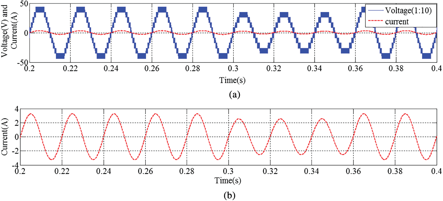
Figure 17: Dynamic results under voltage sag condition (a) Voltage and current (b) Current subsection of (a)

Condition.3 Comparative Study

In this section, a comparative harmonic analysis table between the proposed HES with the traditional approach is presented in Tab. 3. By using the traditional inverter and control approaches, the grid integrated systems are studied in [2,3,7]. In [2], a grid integrated solar and battery system is studied by using a three-level neutral point clamped (NPC) inverter. From the study, it is found that NPC inverter can generate three-level output voltage through the traditional techniques. However, the system lags its performance because of the increasing number of switches, cost, and harmonic aspects as presented in Tab. 3. In [3], a grid-integrated wind energy system is studied by using traditional approaches. It shows the active filter capability even during the shutdown condition of the wind turbine. However, the system lags its performance because of conventional inverter and control strategies, cost, and harmonic aspects as presented in Tab. 3. A similar type of CHBI approach is studied in [7] to generate multiple voltage levels by a reduced number of switches. The THD results of the generated voltage and current are presented in Tab. 3 by using the filter and without the filter. However, due to the traditional controller, the harmonics are quite more as per the IEEE-1549 standards. As a solution, a combined CHBI integrated HES and UCAP based energy storage device-based system is proposed. This indicates that the PQ of HES is enhanced significantly on the point of harmonic and stability analysis. In addition to that, the structure of the HES and developed strategy is simpler than the other discussed topologies [2,3,7]. Most of the cases, the researchers are used LC and LCL filters for filtering operation. However, the HES can eliminate the harmonics and avoid the need for passive filter requirements. Due to this, the cost and size of the HES design are reduced. This shows the need and advancement of the proposed controller and inverter design for real-time applications. Therefore, it is suggested to implement the proposed strategy for real-time renewable power applications.

7  Conclusion

The above study finds that the PQ of HES is improved significantly by using the novel control and HPWM technique based single phase 11-CHBI. In addition to that, the HES can provide excellent power tracking operation through the MP&O technique. The obtained Bode and Nyquist stability curves guaranteed the stability of the proposed control strategy during both steady-state and dynamic conditions. The proposed 11-CHBI requires lesser switches and offers flexible operation during failure of any one of the converters such as solar and wind inverter. 11-CHBI can adjust the voltage levels as per the generation by properly regulating the modulation index. The ANN-PI and Fuzzy-based controller facilitate better dc-link voltage and harmonic regulation irrespective of the system conditions. From the comparative analysis, it is found that by using the traditional controller the harmonics contained in the system is increasing as per the IEEE-1541 standard. To overcome this issue, researchers are preferably used LC and LCL-based passive filters. However, the additional passive devices also increase the size, cost, and provide additional computational burden. Therefore, the proposed strategies provide an optimum solution by reducing the harmonics and eliminating the use of additional passive filter requirements. Looking at the above merits, the suggested approach can be applied for more complex system applications such as three-phase HES, reduced switch multi-level inverter application, electric vehicle stability improvement, and provide faster charging operation. In this manuscript, the achieved and analyzed simulated outputs serve as a basis of a novel control and energy storage approach with increased voltage levels in the solar and wind-based microgrid systems.

Acknowledgement: Assistance provided by Council of scientific and industrial research (CSIR), Government of India, under the acknowledgment number 143460/2K19/1 (File: 09/969(0013)/2020-EMR-I) and Siksha O Anusandhan (Deemed to be University).

Funding Statement: Funding is provided by the Council of scientific and industrial research (CSIR).

Conflicts of Interest: The authors declare that they have no conflicts of interest to report regarding the present study.

Appendix

Solar system data (PV-MF-180TD4): Max power rating (Pmax)-180 W, Open circuit voltage (Voc)-30.4 V, Short circuit current (Isc)-8.03 V, Voltage at max power (Vmp)-24.2 V, Current at max power (Imp)-7.45 V. UCAP parameters (BMOD0165 P048): Rated capacitance-165 F, Minimum capacitance-165 F, Maximum capacitance-200 F, Rated voltage-48 V, Capacitance of individual cells-3,000 F, Number of cells-18, WT and PMSG parameters: Rated power-2 kW, Rated wind speed-10m/s, Radius-1.525 m, Gear ratio-5, Air density-5 m, Height-5 m, Rated power-3 kW, Stator resistance-1.5 Ω, Stator inductance-0.01 mH, Pole pairs-2, Flux-0.2194 Wb, Moment of inertia-2 Kg m.

(a)   Fuzzy logic controller:

(b)   Membership functions-Gaussian-2

(c)   Fuzzy rules’ type-Mamdani

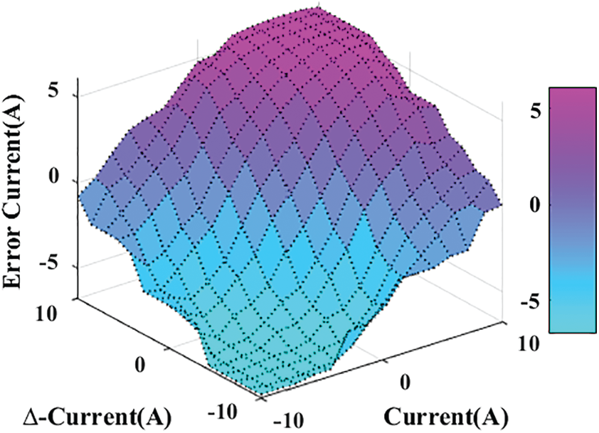
(d)   Rules surface View:

(e)   Defuzzification method-Centroid Method

(f)   The variables’ ranges (domain of discourse):

7 * 7 matrix = 49 rules

large positive (LP), medium positive (MP), small positive (SP), large negative (LN), medium negative (MN), and small negative (SN)

Rules are presented in Tab. 2.

This work is licensed under a Creative Commons Attribution 4.0 International License, which permits unrestricted use, distribution, and reproduction in any medium, provided the original work is properly cited.